Binary Reactive Adsorbate on a Random Catalytic Substrate

Abstract

We study the equilibrium properties of a model for a binary mixture of catalytically-reactive monomers adsorbed on a two-dimensional substrate decorated by randomly placed catalytic bonds. The interacting $A$ and $B$ monomer species undergo continuous exchanges with particle reservoirs and react ($A+B\to\emptyset$) as soon as a pair of unlike particles appears on sites connected by a catalytic bond. For the case of annealed disorder in the placement of the catalytic bonds this model can be mapped onto a classical spin model with spin values $S=-1,0,+1$, with effective couplings dependent on the temperature and on the mean density $q$ of catalytic bonds. This allows us to exploit the mean-field theory developed for the latter to determine the phase diagram as a function of $q$ in the (symmetric) case in which the chemical potentials of the particle reservoirs, as well as the $A-A$ and $B-B$ interactions are equal.

, ,

1 Introduction

Catalytically activated reactions (CARs) involve particles which react only in the presence of another agent acting as a catalyst, and remain chemically inactive otherwise. Usually, the catalyst is part of a solid, inert substrate placed in contact with fluid phases of the reactants, and the reaction takes place only between particles adsorbed on the substrate forming a (dilute) monolayer. These processes are widespread in nature and used in a variety of technological and industrial applications [1].

The work of Ziff, Gulari, and Barshad (ZGB) [2] on the “monomer-dimer” model, introduced as an idealized description of the process of ${\rm CO}$ oxidation on a catalytic surface, as well as the subsequent studies of a simpler “monomer-monomer” reaction model [3], represent an important step in the understanding of CARs properties by revealing the emergence of an essentially collective behavior in the dynamics of the adsorbed monolayer. On two-dimensional (2D) substrates, first- and second-order non-equilibrium phase transitions involving saturated, inactive phases (substrate poisoning, i.e., most of the adsorption sites are occupied by same-type particles) and reactive steady-states have been evidenced and studied in detail [2, 3, 5, 4, 6]. Most of these available studies pertain to idealized homogeneous substrates.

In contrast, the equilibrium properties of the adsorbed monolayer in the case of CARs are much less studied and the understanding of the equilibrium state remains rather limited. Moreover, actual substrates are typically disordered and generically the catalyst is an assembly of mobile or localized catalytic sites or islands [1]; the recently developed artificially designed catalysts [7] involve inert substrates which are decorated by catalytic particles. Theoretical studies which have addressed the behavior of CARs on disordered substrates have been so far focused on the effect of site-dependent adsorption/desorption rates because natural catalysts are, in general, energetically heterogeneous [8, 9]; only few studies, in particular some exactly solvable 1D models of $A+A\to\emptyset$ reactions and a Smoluchowski-type analysis of $d$-dimensional CARs [10], have addressed the case of spatially heterogeneous catalyst distribution.

Recently, we have presented a simple model of a monomer-monomer $A+B\to\emptyset$ reaction on a 2D inhomogeneous, catalyst decorated substrate, and we have shown that for the case of annealed disorder in the placement of the catalytic bonds the reaction model under study can be mapped onto the general spin $S=1$ (GS1) model [12] with effective, temperature dependent couplings [11]. This allows us to exploit the large number of results obtained for the GS1 model [12, 13] in order to elucidate, within a mean-field description [13], the equilibrium properties of the monolayer binary-mixture of reactive monomers on a 2D substrate randomly-decorated by a catalyst.

The organization of the paper is as follows. In Sec. 2 we briefly present the model for a binary-mixture monolayer with an $A+B\stackrel{{\scriptstyle catalyst}}{{\longrightarrow}}\emptyset$ reaction on a 2D inhomogeneous, catalyst decorated substrate and the mapping to a GS1 model; in Sec. 3 we present the mean-field (MF) approximation. Section 4 is devoted to a discussion of the MF phase diagram for the particular cases of a completely catalytic substrate, i.e., $q=1$, and of an inert substrate, i.e., $q=0$, respectively. In Sec. 5 we discuss, on the basis of the results for $q=0$, the MF phase diagram for general values of $q$. We conclude with a brief summary of the results in Sec. 6.

2 Model of a monolayer binary mixture of reactive species on a 2D inhomogeneous, catalyst decorated substrate

We consider a 2D regular lattice (coordination number $z$) of $N$ adsorption sites (Fig. 1), which is in contact with the mixed vapor phase of $A$ and $B$ particles.

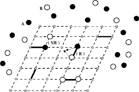
Figure 1: 2D lattice of adsorption sites (small grey circles) in contact with a mixed vapor phase. Black (white) circles denote $A$ ($B$) particles, respectively, solid lines denote “catalytic bonds”. (R): configuration in which an annihilation reaction ($\nearrow\nwarrow$) takes place; (NR): NN pair $A$-$B$, but no reaction because there is no catalytic bond between these sites.

The $A$ and $B$ particles can adsorb onto $vacant$ sites, and can desorb back to the reservoir. The system is characterized by chemical potentials $\mu_{A,B}$ maintained at constant values and measured relative to the binding energy of an occupied site, so that $\mu_{A,B}>0$ corresponds to a preference for adsorption. Both $A$ and $B$ particles have hard cores prohibiting double occupancy of the adsorption sites and nearest-neighbor (NN) attractive $A-A$, $B-B$, and $A-B$ interactions of strengths $J_{A}$, $J_{B}$, and $J_{AB}$, respectively. The occupation of the $i$-th site is described by a “spin” variable

$$\sigma_{i}=\cases{+(-)1,&~{}~{}{site $i$ occupied by $A$ ($B$),}\\ ~{}0,&~{}~{}{site $i$ empty.}\\ }$$ (1)

We assign, at random, to some of the lattice bonds (solid lines in Fig. 1) “catalytic” properties such that if an $A$ and a $B$ particle occupy simultaneously NN sites connected by such a catalytic bond, they instantaneously react and desorb, and the product ($AB$) leaves the system; $A$ and $B$ particles occupying NN sites not connected by a catalytic bond harmlessly coexist, and we assume that the reverse process of a simultaneous adsorption of an $A$ and a $B$ on a catalytic bond has an extremely low probability and can be neglected. The “catalytic” character of the lattice bonds is described by variables $\zeta_{<ij>}$, where $<ij>$ denotes a pair of NN sites $i$ and $j$,

$$\zeta_{<ij>}=\cases{1,&~{}~{}{$<ij>$~{}is a catalytic bond,}\\ 0,&~{}~{}{otherwise,}\\ }$$ (2)

and we take $\{\zeta_{<ij>}\}$ as independent, identically distributed random variables with the probability distribution

$$\varrho(\zeta)=q\delta(\zeta-1)+(1-q)\delta(\zeta).$$ (3)

Note that the probability $q$ that a given bond is catalytic equals the mean density of the catalytic bonds. The two limiting cases, $q=0$ and $q=1$, correspond to an inert substrate and to a homogeneous catalytic one, respectively. We further assume that the condition of instantaneous reaction $A+B\stackrel{{\scriptstyle catalyst}}{{\longrightarrow}}\emptyset$ together with negligible simultaneous adsorption of an $A$ and a $B$ particle on a catalytic bond is formally equivalent to allowing a NN $A-B$ repulsive interaction of strength $\lambda\gg 1$, followed by the limit $\lambda\to\infty$, for $A-B$ pairs connected by catalytic bonds.

As shown in Ref.[11], in thermal equilibrium and for situations in which the disorder in the placement of the catalytic bonds is annealed, i.e., the partition function, rather than its logarithm, is averaged over the disorder, the model under study is mapped exactly onto that of a GS1 model. The ”effective” GS1 Hamiltonian describing the adsorbate at temperature $T$ is:

$$\hskip 14.22636pt\mathcal{H}_{e}=-J\sum_{<ij>}\sigma_{i}\sigma_{j}-K\sum_{<ij>}\sigma_{i}^{2}\sigma_{j}^{2}-C\sum_{<ij>}\left(\sigma_{i}\sigma_{j}^{2}+\sigma_{j}\sigma_{i}^{2}\right)-H\sum_{i=1}^{N}\sigma_{i}+\Delta\sum_{i=1}^{N}\sigma_{i}^{2}\,,$$ (4)

where the coupling constants are given explicitely by:

$$J=\frac{J_{A}+J_{B}-2J_{AB}}{4}-\frac{k_{B}T}{2}\ln(1-q):=J_{0}-\frac{k_{B}T}{2}\ln(1-q)\,,$$

$$K=\frac{J_{A}+J_{B}+2J_{AB}}{4}+\frac{k_{B}T}{2}\ln(1-q):=K_{0}+\frac{k_{B}T}{2}\ln(1-q)\,,$$ (5)

$$C=\frac{J_{A}-J_{B}}{4},\;H=\frac{\mu_{A}-\mu_{B}}{2},\;\Delta=-\frac{\mu_{A}+\mu_{B}}{2},$$

and $T$ is the temperature. In the remaining part of this paper we focus on the symmetric case in which the chemical potentials of the two species are equal, $\mu_{A}=\mu_{B}:=\mu$, (implying $H=0$), and $J_{A}=J_{B}:=j$, (implying $C=0$). This model reduces to the original Blume-Emery-Griffiths (BEG) model [13] in zero magnetic field $H$.

3 Mean-field approximation of the free energy.

The mean-field analysis follows closely the presentation in Ref.[13] and thus here we only briefly outline the main steps. The starting point is the variational principle for the free energy $F$ (see, e.g., Ref.[14])

$$F\leq\Phi[\rho]:=\Tr(\rho\mathcal{H}_{e})+k_{B}T\Tr(\rho\ln\rho)\,$$ (6)

where $\rho$ is any trial density matrix, i.e., $\Tr(\rho)=1$; the equality holds for $\rho=\exp(-\beta\mathcal{H}_{e})/\Tr[\exp(-\beta\mathcal{H}_{e})]$, where $\beta^{-1}=k_{B}T$ and $\Tr$ denotes the sum over all spin configurations.

Within the mean-field approximation the trial density $\rho$ is chosen from the subspace of products of single-site densities, i.e., $\rho=\prod\limits_{i=1}^{N}\rho_{i}$; furthermore restricting to the case of translationally invariant states, i.e., $\rho_{i}$ being independent of $i$, leads to trial densities of the form $\rho=\rho_{1}^{N}$. Note that this last restriction implies that within the present approximation the analysis cannot account for the occurrence of staggered states (i.e., splitting in ordered sub-lattices) and the emphasis is put on the disordered and ordered homogeneous states. The single site density $\bar{\rho}_{1}$ minimizing the functional $\Phi/N$, subject to the constraint $\Tr(\bar{\rho}_{1})=1$, is

$$\bar{\rho}_{1} =\exp(-\beta h)/\Tr[\exp(-\beta h)]\,,$$

$$h =-J^{\prime}M\sigma_{1}+(\Delta-K^{\prime}Q)\sigma_{1}^{2}\,,$$ (7)

where $J^{\prime}=zJ$, $K^{\prime}=zK$, and

$$M:=\langle\sigma_{1}\rangle\equiv\Tr(\bar{\rho}_{1}\sigma_{1})\,,$$

$$Q:=\langle\sigma_{1}^{2}\rangle\equiv\Tr(\bar{\rho}_{1}\sigma_{1}^{2})\,$$ (8)

are the so-called magnetization $M$ and the quadrupolar moment $Q$, respectively. This leads to the following approximation $f_{mf}$ of the free energy per-site:

$$f_{mf}(M,Q)=\Phi[\bar{\rho}_{1}]/N=\frac{1}{2}(J^{\prime}M^{2}+K^{\prime}Q^{2})-\frac{1}{\beta}\ln\left[1+2e^{-\beta\Delta}e^{\beta K^{\prime}Q}\cosh(\beta J^{\prime}M)\right]\,.$$ (9)

Note that in the binary mixture language the values of the magnetization and of the quadrupolar moment [Eq.(8)] represent the difference and the sum (total coverage) of the average densities $n_{A}$ and $n_{B}$ of $A$ and $B$ species, respectively:

$$M=n_{A}-n_{B}\,,\,\,\,Q=n_{A}+n_{B}\,.$$ (10)

For given values of the temperature $T$ and of the field $\Delta=-\mu$ [Eq.(2)], the order parameters $M$ and $Q$ are obtained by solving Eqs.(7) and (8). The pair $(M,Q)$ characterizing the state of the system is selected from the possible solutions as the one which minimizes $f_{mf}$ in Eq.(9) above. Explicitely, the equations determining $M$ and $Q$ are:

$$M=\frac{2\sinh(\beta J^{\prime}M)}{\exp(-\beta\mu-\beta K^{\prime}Q)+2\cosh(\beta J^{\prime}M)}\,,$$ (11)

$$Q=\frac{2\cosh(\beta J^{\prime}M)}{\exp(-\beta\mu-\beta K^{\prime}Q)+2\cosh(\beta J^{\prime}M)}\,.$$ (12)

Note that there is always a solution of these equations with $M=0$, i.e., a disordered state (or, in the language of binary mixtures, a mixed state).

Alternatively, one may search directly for the absolute minimum of the per-site free-energy function with respect to $M$ and $Q$. The values $M$ and $Q$ at the minimum (minima in case of phase equilibria) will define the thermodynamically stable phase(s). While the first formulation is more useful for analytical work, reduced to analyzing the number of solutions of two coupled algebraic equations, the latter is advantageous for numerical calculations. In the following we shall use both of them. Before proceeding we note that $f_{mf}(M,Q)$ [Eq. (9)] is an even function of $M$ (i.e., invariant under the change $M\to-M$), and thus in the following we shall restrict the discussion to the case $M\geq 0$; the states with $M\leq 0$ are immediately obtained via a change of sign. This is a consequence of the symmetry in the chemical potentials ($\mu_{A}=\mu_{B}$) or, in the magnetic language, of a vanishing magnetic field $H=0$. In other words, in the space spanned by $(T,\mu,H)$ the phase diagrams in the plane $H=0$ along the $H=0^{+}$ side and any equilibrium state characterized by $(M>0,Q)$ have corresponding phase diagrams and states $(-M,Q)$ located on the $H=0^{-}$ side.

4 Homogeneous catalytic or catalytically inert substrates.

4.1 The case of a homogeneous catalytic substrate: $q=1$.

The case of a homogeneous, completely catalytic substrate can be studied analytically because of the particular form of the interaction parameters $K^{\prime}$ and $J^{\prime}$. In the limit $q\to 1$, Eq. (2) implies:

$$J^{\prime}=zJ_{0}-z\frac{k_{B}T}{2}\ln(1-q)\stackrel{{\scriptstyle q\to 1}}{{\longrightarrow}}+\infty\,,$$

$$K^{\prime}=zJ_{0}+z\frac{k_{B}T}{2}\ln(1-q)\stackrel{{\scriptstyle q\to 1}}{{\longrightarrow}}-\infty\,,$$ (13)

while $J^{\prime}+K^{\prime}=zj$ remains finite in this limit. The analysis of Eqs.(11) and (12) proceeds as follows. From Eq.(12), the solutions with $M=0$, i.e., disorder states, have the quadrupolar moment

$$Q=\lim_{K^{\prime}\to-\infty}\frac{2}{\exp(-\beta\mu)\exp(-\beta K^{\prime}Q)+2}=0\,,$$ (14)

for any finite temperature and finite chemical potential $\mu$. This corresponds to an empty lattice state.

Taking the ratio of Eqs.(11) and (12) we find that the ordered states, $M\neq 0$, satisfy

$$Q=\lim_{J^{\prime}\to+\infty}M\coth(\beta J^{\prime}M)=|M|\,.$$ (15)

In this limit the substrate is occupied by a single species, either $A$ or $B$ with equal probability. With $K^{\prime}+J^{\prime}=jz$, for any finite temperature and finite chemical potential $M$ is determined from

$$M=\frac{1-\exp(-2\beta J^{\prime}M)}{\exp(\beta\Delta)\exp(-\beta jzM)+1+\exp(-2\beta J^{\prime}M)}$$

$$\stackrel{{\scriptstyle J^{\prime}\to+\infty}}{{\longrightarrow}}\frac{1}{\exp(-\beta\mu)\exp(-\beta jzM)+1}\,.$$ (16)

It is easy to see that Eq.(16) has a solution $0\leq|M|\leq 1$ for any $T>0$ and any $\mu$. Thus, in virtue of Eq.(15), the lattice is occupied, with equal probability, either by $|M|\times N$ particles of species $A$ or by $|M|\times N$ particles of species $B$.

4.2 The case of an inert substrate: $q=0$.

In the case of a catalytically inert substrate, $q=0$, we have

$$J^{\prime}=z\frac{j-2J_{AB}}{2}=zJ_{0}\,\,,\,\,K^{\prime}=z\frac{j+2J_{AB}}{2}=zK_{0}\,,$$ (17)

and thus the model reduces to the classical BEG model, whose mean-field approximation has been analyzed in detail in Ref. [13]. In the following we briefly summarize the main aspects of the phase diagram of the BEG model such that in the general case $q\neq 0$ we can isolate the effects solely due to the disordered distribution of the catalyst. Moreover, as will be shown in the next section, the equilibrium properties of the adsorbate in the general case $q\neq 0$ can be easily rationalized from the ones on the inert substrate.

First we note that for non-interacting particles, i.e., for $j=J_{AB}=0$ so that $J^{\prime}=K^{\prime}=0$, Eq.(11) implies that $M=0$, and thus Eq.(12) leads to

$$Q=\frac{2}{\exp(-\beta\mu)+2}\,\,,\,n_{A}=n_{B}=Q/2=\frac{\mathfrak{f}}{1+2\mathfrak{f}}\,,$$ (18)

where $\mathfrak{f}:=\exp(\beta\mu)$ is the fugacity, rendering the classical Langmuir adsorption result.

For the case of non-zero interaction parameters $j$ and $J_{AB}$, only the qualitative features of the phase-diagram can be analytically derived (for details see Ref.[13]); here we shall present phase diagrams obtained via direct numerical minimization of the free energy function $f_{mf}$ [Eq.(9)]. Using $zJ_{0}$ as energy scale, the system is characterized by the parameter $\kappa_{0}:=K^{\prime}/J^{\prime}=K_{0}/J_{0}$, the scaled temperature (thermal energy) $t$, and the scaled chemical potential $u$:

$$t:=k_{B}T/(zJ_{0})\,\,,\,u:=\mu/(zJ_{0})\,\,.$$ (19)

We shall discuss below the phase diagrams, as well as the behavior of the order parameters $M$ and $Q$, in the $u-t$ plane at given values of $\kappa_{0}\geq 0$. The reason for the latter restriction is that for sufficiently negative values $\kappa_{0}<\kappa_{0}^{(tr)}<0$, where $\kappa_{0}^{(tr)}$ is a threshold value, it is known that the system will split into ordered sub-lattices [15]. However, such states are not captured by the present formulation of the mean-field equations which assume translational invariance.

Before proceeding with the numerical analysis, we list several general features of the phase diagram that can be obtained from the analysis of Eqs.(11) and (12).
(i) For $M\neq 0$, Eq.(11) can be written as

$$\underbrace{2[tx\cosh(x)-\sinh(x)]}_{\hskip 28.45274pt:=g_{1}(x;t)}+\underbrace{tx\exp(-u/t)\exp(-\kappa_{0}Q/t)}_{\hskip 36.98866pt:=g_{2}(x;t,u)}=0\,,$$ (20)

where $0<x:=M/t\leq 1/t$. Since $g_{1}(x;t>1)$ is a strictly increasing function of $x$, it follows that $g_{1}(x>0;t>1)>g_{1}(0;t>1)=0$; moreover, one has $g_{2}(x>0;t>0,u)>0$, from which one can conclude that for $t>1$ Eq.(20) has only the solution $x=0$, i.e., there are no ordered states for $t>1$.
(ii) For $\mu<\mu_{c}(T)<0$, the positive term $g_{2}(x;t,u<0)$ dominates over the term $g_{1}(x;t)$, which is bounded from below, and thus in this range Eq. (20) has only the solution $x=0$, i.e., there are no ordered states for $u<u_{c}(t)<0$. This is an intuitive result: $\mu<0$ corresponds to a preference for desorption; thus at low negative chemical potential the substrate is covered by a low density two-dimensional gas (which is a mixed phase).
(iii) For $\mu\to\infty$ and finite temperatures, $g_{2}(x;t,u\to\infty)\to 0$, and thus Eq.(20) reduces to $g_{1}(x;t)=0$ which is equivalent to $\tanh(x)=tx$. It follows that for $t<1$ there is always a unique solution $x(t)>0$, and therefore there is an ordered state $M(t<1,\mu\to\infty)\neq 0$ such that $M(t\nearrow 1,\mu\to\infty)\to 0$, i.e., if there is a phase transition at $t=1$ (for $\mu\to\infty$), it is a continuous order-disorder transition.
(iv) In the case of disordered states (i.e., $M=0$) Eq.(12) reduces to

$$\underbrace{2ty+ty\exp(-u/t)\exp(-\kappa_{0}y)-2}_{\hskip 34.14322pt:=g_{3}(y;u,t)}=0\,,$$ (21)

where $0<y:=Q/t\leq 1/t$. For $\mu>0$ and finite temperatures, $g_{3}(y;u>0,t)$ is a strictly increasing function of $y$, and thus Eq. (21) has an unique solution, i.e., in the region $\mu>0$ there are no phase transitions between disordered states.

We now turn to a detailed discussion of the phase diagrams. The most complicated behavior occurs for intermediate values of $\kappa_{0}$, e.g., $\kappa_{0}\simeq 3$ [13]. For $\kappa_{0}=3.0$, in Fig. 2 we show (color coded) the order parameters $M=|n_{A}-n_{B}|$ and $Q=n_{A}+n_{B}$, as well as the lines corresponding to the various phase transitions composing the phase diagram.

                          (a) [M]                                                 (b) [Q]

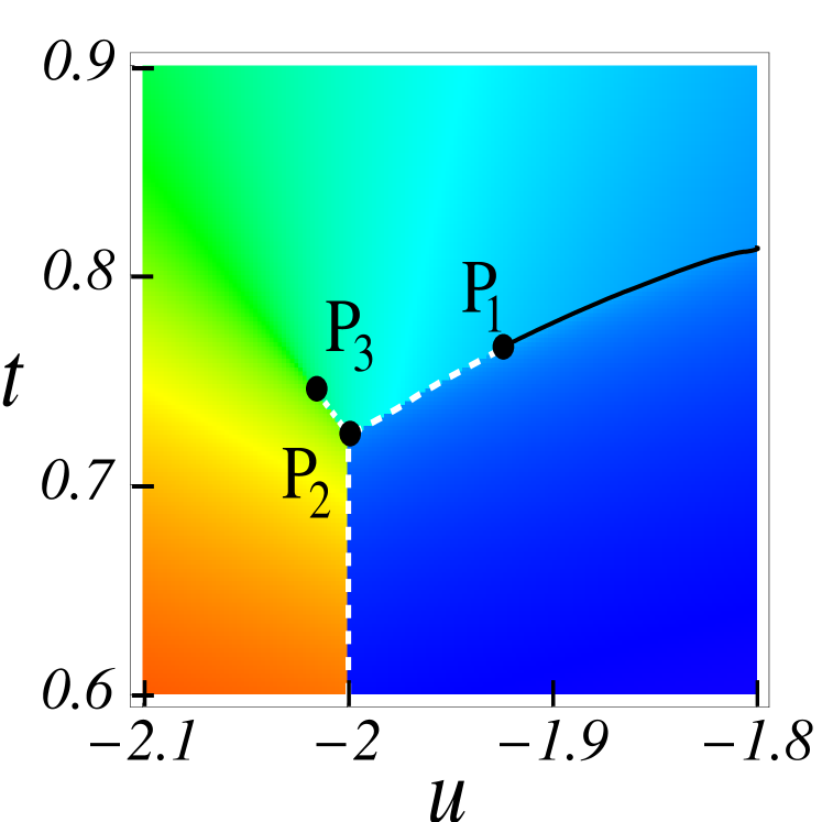
Figure 2: (a) Magnetization $M$ and (b) quadrupolar moment $Q$ for an inert substrate ($q=0$) as functions of $t:=k_{B}T/(zJ_{0})$ and $u:=\mu/(zJ_{0})$ for $\kappa_{0}=3.0$. The color coding (shown at the right) is the same for both figures, and linearly interpolates between zero (red) and one (dark blue) via yellow, green, and light blue. $P_{1}$ is a tricritical point, $P_{2}$ is a quadruple point, and $P_{3}$ is a critical end point. Solid black lines are lines of critical points and indicate second-order phase transitions, while the dashed white lines are lines of triple points indicating first-order transitions.

At low temperatures, i.e. $t\leq t_{P_{2}}\simeq 0.72$ and low negative chemical potential, i.e., $u<<u_{P_{2}}\simeq-2.0$, the substrate is covered by a very low density, two-dimensional mixed gas ($M=0$, $Q\ll 1$), in agreement with (ii) above. Increasing the chemical potential $u$ at fixed temperature $t<t_{P_{2}}$, the system undergoes a first-order phase transition at $u=u_{c}(t)\simeq-2.0$ (the white dashed line located at $u_{c}(t)\simeq-2.0$) upon which the density of the monolayer increases abruptly to almost one [as indicated by the dark blue color in Fig. 2(b)] and the monolayer also (partially) demixes, i.e. $0<M\leq Q$ [as indicated by the lighter blue or green color in Fig. 2(a)]. Thus in the region $u>u_{c}(t)$ as anticipated in (iv) above the substrate is covered by a dense $A$-rich monolayer (for $H=\mu_{A}-\mu_{B}\to 0^{+}$; with equal probability, a dense $B$-rich monolayer forms for $H=\mu_{A}-\mu_{B}\to 0^{-}$). Therefore this first-order transition line, which is located at almost constant $\mu\simeq-2.0$ and extends from $P_{2}$ to $t\to 0$, is a line of triple points.

We focus now on the region $u>u_{c}(t)$. At constant $u$, upon approaching from below the line $P_{2}$-$P_{1}$, which continues to $u\to\infty$, the demixing is less and less pronounced. Increasing the temperature at fixed $u\geq u_{P_{1}}$, upon crossing the line starting at $P_{1}$ (solid black line in Fig. 2) the dense $A$-rich (or $B$-rich) monolayer undergoes a second-order phase transition (both $M$ and $Q$ are changing continuously there; note in Fig. 2(a) the thin band of yellow color, which ends at $P_{1}$, corresponding to very small but non-zero values of $M$) such that at high temperatures the substrate is covered by a mixed dense monolayer. As discussed in (i) and (iii) above, this line of critical points stays below $t=1$ for all values of $u$, and it approaches $t=1$ for $u\to\infty$. Upon crossing the line segment $P_{2}$-$P_{1}$ (white dashed line) the transition from the dense $A$-rich (or $B$-rich) monolayer to the dense mixed monolayer is of first order with a jump in both coverage and composition, i.e., in both $Q$ and $M$ (using the color code, for $M$ this is indicated by the transition from red to green, without yellow in between, while for $Q$ by the direct transition from dark blue to light-blue and green). The line segment $P_{2}$-$P_{1}$ is also a line of triple points since there three phases coexist: dense $A$-rich, dense $B$-rich, and dense mixed monolayer, respectively.

For $u<u_{c}(t)$, upon crossing (from below) the line $P_{2}-P_{3}$ the system undergoes a first-order transition from a low density mixed monolayer to a higher density mixed monolayer: there is a jump in the coverage, i.e., $Q$ varies discontinuously [as indicated in Fig. 2(b) by the color change from light green to light blue (without dark green in between)], while $M$ remains zero. The jump in $Q$ upon crossing the line $P_{2}-P_{3}$ decreases as the crossing point approaches $P_{3}$, and it becomes zero at $P_{3}$. Thus $P_{3}$ is a critical point. Note that for temperatures $t$ such that $t_{P_{2}}<t<t_{P_{3}}$, e.g., $t=0.73$, increasing $u$ at constant temperature from small negative values toward positive values will drive the state of the monolayer from the mixed gas phase towards the $A$-rich (or $B$-rich) dense phase via two consecutive first-order phase transitions, corresponding to crossing the line $P_{2}-P_{3}$ (with a jump only in $Q$) followed by crossing the line $P_{2}-P_{1}$ (with a jump in both $Q$ and $M$).

The point $P_{1}$ is a tricritical point (it belongs also to the critical lines of the $A$-rich dense phase $\to$ mixed gas and $B$-rich dense phase $\to$ mixed gas transitions). $P_{2}$ is a quadruple point, i.e., at $P_{2}$ four phases coexist: dense $A$-rich, dense $B$-rich, dense mixed, and dilute mixed monolayer, respectively

Varying $\kappa_{0}$ will lead to topological changes only near the points $P_{1}$, $P_{2}$, $P_{3}$ as follows. For $\kappa_{0}\ll 1$, the line $P_{2}$-$P_{3}$ and thus the point $P_{2}$ do not occur [there is no jump in the total coverage if the density is increased while keeping the monolayer mixed, i.e., in that region which is red in Fig. 2(a)], so that at the tricritical point $P_{1}$ the line of triple points connects directly with the one corresponding to the second-order phase transitions. With increasing $\kappa_{0}$, the line $P_{2}$-$P_{3}$ emerges, and for $\kappa_{0}\lesssim 3$ the behavior is the same as the one at $\kappa_{0}=3$. For $\kappa_{0}\gtrsim 3$ the only change is that the point $P_{3}$ is located at higher values of $t$ than $P_{1}$. With increasing $\kappa_{0}>3$ $P_{1}$ is shifting towards $P_{2}$ and eventually reaches the first-order triple line such that for large $\kappa_{0}$, e.g., $\kappa_{0}\gtrsim 5$, $P_{1}$ (which at low and medium values of $\kappa_{0}$ is a tricritical point) merges with $P_{2}$ forming a critical end point.

5 The case of a disordered substrate: $0<q<1$.

In the case of a disordered substrate, $0<q<1$, one has

$$J^{\prime}=zJ_{0}-\frac{zk_{B}T}{2}\ln(1-q)\,,$$

$$K^{\prime}=zK_{0}+\frac{zk_{B}T}{2}\ln(1-q)\,.$$ (22)

Using again $zJ_{0}$ as the energy scale, the system is now characterized by the two variables $t$ and $u$ defined in Subsec. 4.2, a disorder parameter $\bar{q}$ defined as

$$\bar{q}=1-(1-q)^{z}\,,\mathrm{~{}i.e.,~{}}z\ln(1-q)=\ln(1-\bar{q})\,,$$ (23)

and the parameter

$$\kappa(t,\bar{q}):=K^{\prime}/J^{\prime}=\frac{2\kappa_{0}+t\ln(1-\bar{q})}{2-t\ln(1-\bar{q})}\,.$$ (24)

Here we indicated explicitely that now the ratio $\kappa$ depends both on the temperature and on the disorder parameter $\bar{q}$.[Note that $\kappa(t,0)=\kappa(0,\bar{q})=\kappa_{0}$.] Therefore, we shall discuss the phase diagrams, as well as the behavior of the order parameters $M$ and $Q$, in the $u-t$ plane for given values of $\kappa_{0}$ and $\bar{q}$.

Eq.(24) implies that for any given $0<\bar{q}<1$ and $\kappa_{0}>0$, the ratio $\kappa(t,\bar{q})$ becomes negative at high enough temperatures, i.e., $\kappa(t>t_{tr},\bar{q})<0$, where the threshold temperature $t_{tr}$ is given by

$$t_{tr}(\bar{q};\kappa_{0})=2\kappa_{0}/|\ln(1-\bar{q})|\,;$$ (25)

note that for a given $\kappa_{0}$, i.e., for a given mixture, $t_{tr}$ is a decreasing function of $\bar{q}$. As already mentioned, for sufficiently negative values of $\kappa$ the system splits into ordered sub-lattices [15], which generally leads to a significant decrease in the yield of the catalytic reaction. Using $t_{tr}$ as a measure of this tendency, Eq.(25) implies that it is desirable to run the reaction at low enough temperatures in order to maintain a mixed monolayer, and that this range of temperatures decreases with an increasing mean density of catalytic bonds.

At constant temperature, and for fixed values of $\bar{q}$ and of $\kappa_{0}$, the parameter $\kappa(t,\bar{q})$ is constant; for two temperatures $t_{1}$ and $t_{2}>t_{1}$, it satisfies $\kappa(t_{2}>t_{1},\bar{q})<\kappa(t_{1},\bar{q})$ (in particular, one has $\kappa(t,\bar{q})\leq\kappa_{0}$). Thus, for any chosen temperature $\bar{t}\leq t_{tr}(\bar{q};\kappa_{0})$ the isotherms $M(\bar{t},u)$ and $Q(\bar{t},u)$ can be simply read as the ones corresponding to an inert substrate, as in Subsec. 4.2, at the same temperature $\bar{t}$ but for a binary mixture with $\bar{\kappa}_{0}=\kappa(\bar{t},\bar{q})<\kappa_{0}$. Since larger values of $\bar{t}$ correspond to smaller values of $\bar{\kappa}_{0}$, the phase diagram is expected to be more similar to one at low $\kappa_{0}$ on an inert substrate, and thus only the first-order mixed gas $\to$ $A$-rich ($B$-rich) dense monolayer transition and the second-order transition lines joining at a tricritical point are generally present. The tricritical point $P_{1}$ shifts towards increasing values of $u$ with increasing $\bar{q}$, and the first-order transition line is a smooth curve (rather than consisting of two segments $P_{2}-P_{1}$ and $P_{2}\to$ zero temperature), which runs from $u\simeq-2.0$ at low temperature (corresponding to the location in the case $\kappa_{0}$) to $P_{1}$. These qualitative features can be seen in Figs. 3 and 4 where we show results corresponding to $\kappa_{0}=3.0$ for $\bar{q}=0.3$ and $\bar{q}=0.6$, respectively, which allows one a direct comparison with the phase diagram on the inert substrate. Note that in these cases the threshold temperatures [Eq.(25)] for splitting into ordered sub-lattices are very high [$t_{tr}(0.3;0.3)\simeq 16.8$, $t_{tr}(0.6;0.3)\simeq 6.54$], thus the present version of the mean-field analysis is justified in the range $t\leq 1$ we are interested in.

                          (a) [M]                                                 (b) [Q]

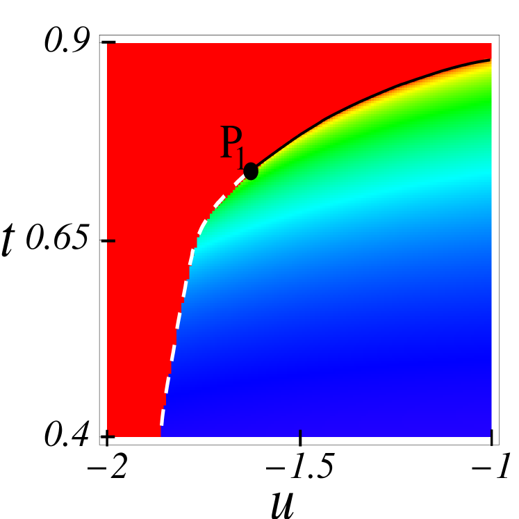
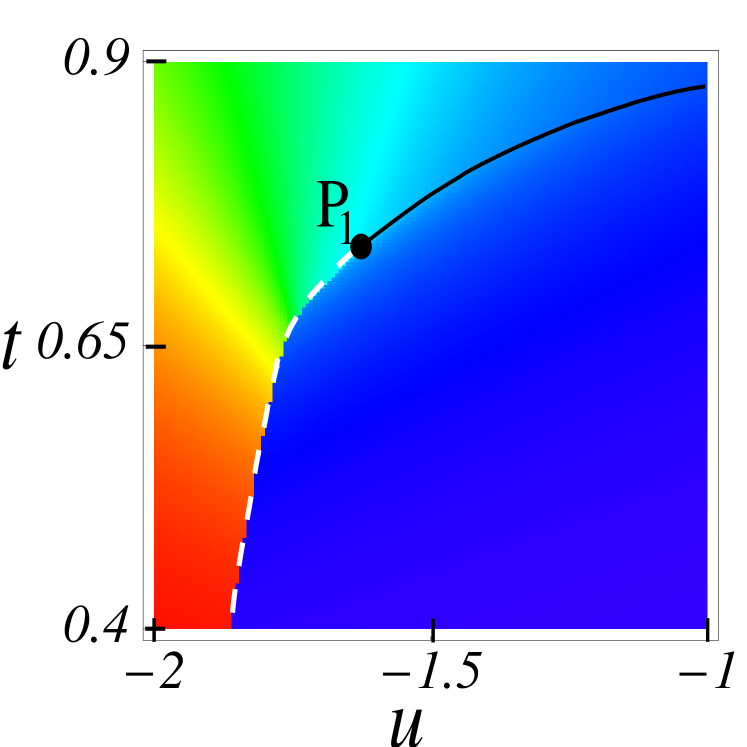
Figure 3: (a) Magnetization $M$ and (b) quadrupolar moment $Q$ as functions of $t:=k_{B}T/(zJ_{0})$ and $u:=\mu/(zJ_{0})$ for $\kappa_{0}=3.0$ and $\bar{q}=0.3$. The color coding (shown at the right) is the same for both figures, and linearly interpolates between zero (red) and one (dark blue) via yellow, green, and light blue. Solid black lines are lines of critical points and indicate second-order phase transitions, while the dashed white lines are lines of triple points indicating first-order transitions.

                          (a) [M]                                                 (b) [Q]

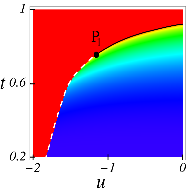
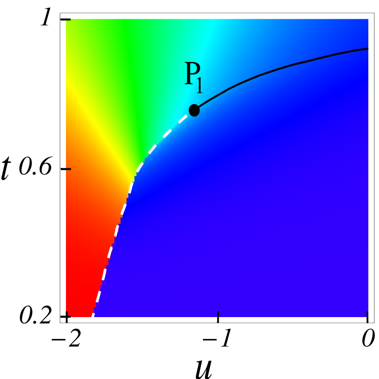
Figure 4: Same as Fig. 3 for $\bar{q}=0.6$.

For an efficient catalytic reaction, the system would have to be operated such that the substrate is covered by a mixed, not too dilute monolayer, i.e., not too low positive chemical potential and temperatures above the second-order transition line, i.e., $t\simeq 1.0$, but below the threshold temperature $t_{tr}(\bar{q};\kappa_{0})$ for which the splitting into ordered sublattices may occur. For a given binary mixture, i.e., given $\kappa_{0}$, the requirement $t_{tr}<1$ implies an upper bound $\bar{q}_{op}$ on the mean density of catalytic bonds, i.e.,

$$t_{tr}<1\Rightarrow\bar{q}<\bar{q}_{op}=1-\exp(-2\kappa_{0})\,.$$ (26)

This is somewhat surprising: a substrate which is only partially decorated by the catalyst, i.e., $\bar{q}<\bar{q}_{op}<1$, would be the optimal choice because it avoids transitions into a passive state (poisoned substrate). For binary mixtures with small values of $\kappa_{0}$ the upper bound given above implies a drastic constraint (e.g., at $\kappa_{0}=0.5$, $\bar{q}_{op}\simeq 0.63$), while for binary mixtures with large values of $\kappa_{0}$, the above constraint is basically irrelevant (e.g., at $\kappa_{0}=3.0$, $\bar{q}_{op}\simeq 0.998$).

6 Summary

Within a mean-field approach we have studied the equilibrium properties of a model for a binary mixture of catalytically-reactive monomers adsorbed on a two-dimensional substrate, decorated by randomly placed catalytic bonds of mean density $q$. Our analysis here has been focused on annealed disorder in the placement of the catalytic bonds and on the symmetric case in which the chemical potentials $\mu_{A}$ and $\mu_{B}$, as well as the interactions $J_{A}$ and $J_{B}$ of the two species, are equal.

We have shown that in the general case $0<q<1$ the mean-field phase diagram and the behavior of the composition $n_{A}-n_{B}$ and of the total coverage $n_{A}+n_{B}$ can be extracted from the corresponding results on an inert substrate ($q=0$). We have determined certain restrictions on the temperature, at which the system is operated, as well as a somewhat surprising upper bound $q_{op}$ of the density of catalytic bonds, which have to be obeyed in order to maintain the monolayer in a mixed and thus active state. Even in this highly symmetric case studied here, the phase diagrams are rather rich, containing, e.g., lines of second-order phase transitions and tricritical points. We have pointed out the likely occurrence of staggered phases at intermediate temperatures.

Finally, we note that in the generic case in which $\mu_{A}\neq\mu_{B}$ and $J_{A}\neq J_{B}$, the behavior is expected to be even richer (see, e.g., Ref. [16] for a detailed discussion of the phase diagrams for the general spin $S=1$ model). These aspects, as well as the issue of staggered phases or that of quenched disorder, are left for future work.

References

References

- [1] Bond G C 1987 Heterogeneous Catalysis: Principles and Applications (Oxford: Clarendon); Avnir D, Gutfraind R and Farin D 1994 Fractals in Science, ed Bunde A and Havlin S (Berlin: Springer) p 229
- [2] Ziff R M, Gulari E and Barshad Y 1986 Phys. Rev. Lett.. 56 2553
- [3] Ziff R M and Fichthorn K 1986 Phys. Rev.B 34 2038; Fichthorn K, Gulari E and Ziff R M 1989 Phys. Rev. Lett.63 1527; Meakin P and Scalapino D 1987 J. Chem. Phys.87 731; Zhuo J and Redner S 1993 Phys. Rev. Lett.70 2822
- [4] Jensen I, Fogedby H C and Dickman R 1990 Phys. Rev.A 41 3411
- [5] see, e.g., Albano E V 1992 Phys. Rev. Lett.69 656; Considine D, Redner S and Takayasu H 1989 Phys. Rev. Lett.63 2857; Evans J W and Ray T R 1993 Phys. Rev.E 47 1018; Krapivsky P L 1992 Phys. Rev.A 45 1067; Krapivsky P L 1995 Phys. Rev.E 52 3455; Kim M H and Park H 1994 Phys. Rev. Lett.73 2579; Monetti R A 1998 Phys. Rev.E 58 144; Argyrakis P, Burlatsky S F, Clément E and Oshanin G, Phys. Rev.E 63 021110
- [6] Marro J and Dickman R 1999 Nonequilibrium Phase Transitions in Lattice Models (Cambridge: Cambridge University)
- [7] Abbet S, Sanchez A, Heiz U, Schneider W -D, Ferrari A M, Pacchioni G and Rösch N 2000 Surf. Sci. 454-456 984
- [8] Henry C 1998 Surf. Sci. Rep. 31 235; Larsen J H and Chorkendorff I 1999 Surf. Sci. Rep. 35 163
- [9] see, e.g., Frachebourg L, Krapivsky P L and Redner S 1995 Phys. Rev. Lett.75 2891; Hoenicke G L and Figueiredo W 2000 Phys. Rev.E 62 6216; Hua D and Ma Y 2002 Phys. Rev.E 66 066103
- [10] Oshanin G and Burlatsky S F 2002 J. Phys. A: Math. Gen.35 L695; Oshanin G and Burlatsky S F 2003 Phys. Rev.E 67 016115; Oshanin G, Benichou O and Blumen A 2003 Europhys. Lett. 62 69; Oshanin G, Benichou O and Blumen A 2003 J. Stat. Phys. 112 541; Oshanin G and Blumen A 1998 J. Chem. Phys.108 1140; Toxvaerd S 1998 J. Chem. Phys.109 8527
- [11] Oshanin G, Popescu M N and Dietrich S 2004 Phys. Rev. Lett.93 020602
- [12] see, e.g., Berker A N and Wortis M 1976 Phys. Rev.B 14 4946; Lawrie I D and Sarbach S 1984 Phase Transitions and Critical Phenomena vol 9 ed Domb C and Lebowitz J L (New York: Academic) p 2; Ananikian N S, Avakian A R and Izmailian N Sh 1991 Physica A 172 391; Mi X D and Yang Z R 1995 J. Phys. A: Math. Gen.28 4883; and references therein
- [13] Blume M, Emery V J and Griffiths R B 1971 Phys. Rev.A 4 1071; Bartis J 1973 J. Chem. Phys.59 5423; Mukamel D and Blume M 1974 Phys. Rev.A 10 610; Furman D, Dattagupta S and Griffiths R B 1971 Phys. Rev.B 15 441
- [14] Falk H 1970 Am. J. Phys. 38 991
- [15] William H and Berker A N 1991 Phys. Rev. Lett.67 1027
- [16] Dietrich S and Latz A 1989 Phys. Rev.B 40 9204; Getta T and Dietrich S 1993 Phys. Rev.E 47 1856