Dynamical and thermal effects in nanoparticle systems driven by a rotating magnetic field

Abstract

We study dynamical and thermal effects that are induced in nanoparticle systems by a rotating magnetic field. Using the deterministic Landau-Lifshitz equation and appropriate rotating coordinate systems, we derive the equations that characterize the steady-state precession of the nanoparticle magnetic moments and study a stability criterion for this type of motion. On this basis, we describe (i) the influence of the rotating field on the stability of the small-angle precession, (ii) the dynamical magnetization of nanoparticle systems, and (iii) the switching of the magnetic moments under the action of the rotating field. Using the backward Fokker-Planck equation, which corresponds to the stochastic Landau-Lifshitz equation, we develop a method for calculating the mean residence times that the driven magnetic moments dwell in the up and down states. Within this framework, the features of the induced magnetization and magnetic relaxation are elucidated.

I INTRODUCTION

The study of the dynamics of the nanoparticle magnetic moments and their stability with respect to reorientations is a problem of prominent theoretical and practical importance. In fact, it is related to the stochastic and nonlinear dynamics and to the thermal stability of the magnetic moments in nanoparticle devices including magnetic storage ones. PEW ; DFT At low temperatures, when thermal fluctuations are negligible, the main interest is in the dynamics and stability in time-dependent external magnetic fields. In this case, the problem is usually reduced to the search for solutions of the deterministic Landau-Lifshitz equationLL and to the analysis of their stability. These investigations are also strongly motivated by the possibility of fast switching of the nanoparticle magnetic moments.BWH ; ABB ; BFH ; KR ; SCC ; SW

Due to thermal fluctuations, the dynamics of the nanoparticle magnetic moments becomes stochastic and nonzero probabilities of their transition from one stable state to another appear. In this case, the dynamics can be described by the Fokker-Planck equation that corresponds to the stochastic Landau-Lifshitz equation.B At present this approach is widely used for studying magnetic properties of nanoparticle systems at finite temperatures, including magnetic relaxation.B ; KG ; CCK ; G ; GL ; DT ; DLT

In this paper, we use the deterministic and the stochastic Landau-Lifshitz equations to study some effects induced by the rotating magnetic field in systems of purely deterministic and weakly superparamagnetic nanoparticles. More precisely, we are interested in the effects that arise from the different dynamical states of the up and down magnetic moments. These states are generated by the magnetic field rotating in the plane perpendicular to the up-down axis and they are different even if the static magnetic field along this axis is absent. The reason is that the magnetic moments have a well-defined direction (counterclockwise) of the natural precession, and so the rotating field effectively interacts only with the up or down magnetic moments. We note in this context that some properties of the solutions of the deterministic Landau-Lifshitz equation were previously considered in the context of ferromagnetic resonance,W nonlinear magnetization dynamics,TJS ; BSM and switching of magnetization in cylinders K and spherical nanoparticles.MBSM But, to the best of our knowledge, the above mentioned effects have not been investigated before.

The paper is organized as follows. In Sec. II, we describe the model and the underlying assumptions. In Sec. III, we reduce the deterministic Landau-Lifshitz equation to the algebraic equations that describe the steady-state forced precession of the nanoparticle magnetic moments and derive a criterion of its stability. In the same section, we apply the results for studying the small-angle precession and switching of the magnetic moments. The effects in nanoparticle systems that arise from the simultaneous action of the thermal fluctuations and rotating field are considered in Sec. IV. Here we calculate the mean residence times that the driven magnetic moments reside in the up and down states, and apply these results to study the induced magnetization and magnetic relaxation in nanoparticle systems. We summarize our findings in Sec. V. Finally, in the Appendix we specify the used coordinate systems.

II DESCRIPTION OF THE MODEL

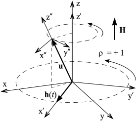
Figure 1: Schematic representation of the model and the used coordinate systems.

We consider a uniaxial ferromagnetic nanoparticle with spatially uniform magnetization which is characterized by the anisotropy field $H_{a}$ and the magnetic moment $\mathbf{m}=\mathbf{m}(t)$ of fixed length $|\mathbf{m}|=m$. The assumption of uniform magnetization is valid for uniform nanoparticles if the exchange length, i.e., the length scale below which the exchange interaction is predominant (for typical magnetic recording materials its order of magnitude is 5–10 nm), exceeds the nanoparticle size. In other cases, e.g., for coated nanoparticles, it can be considered as a first approximation. We assume also that the static magnetic field $\mathbf{H}$ is applied along the easy axis of magnetization (the $z$ axis), and the circularly polarized magnetic field $\mathbf{h(t)}$ is applied in the $xy$ plane (see Fig. 1), i.e., $\mathbf{H}=H\mathbf{e}_{z}$ and

$$\mathbf{h}(t)=h\cos(\omega t)\mathbf{e}_{x}+\rho h\sin(\omega t)\mathbf{e}_{y}.$$ (1)

Here $\mathbf{e}_{x}$, $\mathbf{e}_{y}$, and $\mathbf{e}_{z}$ are the unit vectors along the corresponding axes of the Cartesian coordinate system $xyz$, $h=|\mathbf{h}(t)|$, $\omega$ is the frequency of rotation of $\mathbf{h}(t)$, and $\rho=-1$ or $+1$ that corresponds to the clockwise or counterclockwise rotation of $\mathbf{h}(t)$, respectively. We write the magnetic energy of such a nanoparticle as

$$W=-\frac{H_{a}}{2m}m_{z}^{2}-Hm_{z}-\mathbf{m}\cdot\mathbf{h}(t),$$ (2)

where $m_{z}=\mathbf{m}\cdot\mathbf{e}_{z}$ is the $z$ component of $\mathbf{m}$, and the dot denotes the scalar product.

In the deterministic case, we describe the dynamics of the nanoparticle magnetic moment by the Landau-Lifshitz equationLL

$$\dot{\mathbf{m}}=-\gamma\mathbf{m}\times\mathbf{H}_{eff}-\frac{\lambda\gamma}{m}\,\mathbf{m}\times(\mathbf{m}\times\mathbf{H}_{eff}).$$ (3)

Here $\gamma(>0)$ is the gyromagnetic ratio, $\lambda(>0)$ is the dimensionless damping parameter, the cross denotes the vector product, and

$$\mathbf{H}_{eff}=-\frac{\partial W}{\partial\mathbf{m}}=\mathbf{h}(t)+\bigg{(}H_{a}\frac{m_{z}}{m}+H\bigg{)}\mathbf{e}_{z}$$ (4)

is the effective magnetic field acting on $\mathbf{m}$.

If the magnetic moment interacts with a heat bath, we use the stochastic Landau-Lifshitz equationB

$$\dot{\mathbf{m}}=-\gamma\mathbf{m}\times(\mathbf{H}_{eff}+\mathbf{n})-\frac{\lambda\gamma}{m}\,\mathbf{m}\times(\mathbf{m}\times\mathbf{H}_{eff}),$$ (5)

where $\mathbf{n}=\mathbf{n}(t)$ is the thermal magnetic field with zero mean and correlation functions $\langle n_{\alpha}(t_{1})n_{\beta}(t_{2})\rangle=2\Delta\delta_{\alpha\beta}\delta(t_{2}-t_{1})$, $n_{\alpha}(t)$ ($\alpha=x,y,z$) are the Cartesian components of $\mathbf{n}(t)$, $\Delta=\lambda k_{B}T/\gamma m$ is the intensity of the thermal field, $k_{B}$ is the Boltzmann constant, $T$ is the absolute temperature, $\delta_{\alpha\beta}$ is the Kronecker symbol, $\delta(t)$ is the Dirac $\delta$ function, and the angular brackets denote averaging with respect to the sample paths of $\mathbf{n}(t)$. According to Eq. (5), the conditional probability density $P=P(\theta,\varphi,t|\theta^{\prime},\varphi^{\prime},t^{\prime})$ ($t\geq t^{\prime}$) that describes the statistical properties of $\mathbf{m}$ in the terms of the polar $\theta$ and azimuthal $\varphi$ angles, satisfies the (forward) Fokker-Planck equationB ; DY

$$\frac{\partial}{\partial t}P\! = \!-\frac{\partial}{\partial\theta}(f_{1}+\gamma^{2}\Delta\cot\theta)P+\gamma^{2}\Delta\frac{\partial^{2}}{\partial\theta^{2}}P$$ (6)

$$\!-\,\frac{\partial}{\partial\varphi}f_{2}P+\frac{\gamma^{2}\Delta}{\sin^{2}\theta}\frac{\partial^{2}}{\partial\varphi^{2}}P$$

with

$$\begin{array}[]{c}f_{1}=-\displaystyle\frac{\gamma}{m\sin\theta}\left(\lambda\sin\theta\frac{\partial}{\partial\theta}+\frac{\partial}{\partial\varphi}\right)W,\\[16.0pt] f_{2}=\displaystyle\frac{\gamma}{m\sin^{2}\theta}\left(\sin\theta\frac{\partial}{\partial\theta}-\lambda\frac{\partial}{\partial\varphi}\right)W.\end{array}$$ (7)

III DYNAMICAL EFFECTS

III.1 Equations for the forced precession

To study the forced precession of the nanoparticle magnetic moment and its stability with respect to small perturbations, we use the Landau-Lifshitz equation (3) and represent $\mathbf{m}(t)$ in the form

$$\mathbf{m}(t)=\mathbf{m}_{0}(t)+\mathbf{m}_{1}(t),$$ (8)

where $\mathbf{m}_{0}(t)$ describes the steady-state precession of $\mathbf{m}(t)$, and $\mathbf{m}_{1}(t)$ is a small deviation from $\mathbf{m}_{0}(t)$. Since $|\mathbf{m}(t)|=|\mathbf{m}_{0}(t)|=m$, it is convenient to introduce the unit vector $\mathbf{u}=\mathbf{m}_{0}(t)/m$ and a small dimensionless vector $\mathbf{v}=\mathbf{m}_{1}(t)/m$ ($v=|\mathbf{v}|\ll 1$). According to this, we decompose the effective magnetic field (4) into the zeroth-order (in $v$) vector

$$\mathbf{H}_{eff}^{(0)}=\mathbf{h}(t)+(H_{a}u_{z}+H)\mathbf{e}_{z}$$ (9)

and the first-order one

$$\mathbf{H}_{eff}^{(1)}=H_{a}v_{z}\mathbf{e}_{z}.$$ (10)

Substituting Eq. (8) and the effective field $\mathbf{H}_{eff}=\mathbf{H}_{eff}^{(0)}+\mathbf{H}_{eff}^{(1)}$ into Eq. (3) and keeping the terms of the zeroth order, we end up with the following equation for $\mathbf{u}$:

$$\dot{\mathbf{u}}=-\gamma\mathbf{u}\times\mathbf{H}_{eff}^{(0)}-\lambda\gamma\mathbf{u}\times(\mathbf{u}\times\mathbf{H}_{eff}^{(0)}).$$ (11)

Introducing, as usual, the rotating Cartesian coordinate system $x^{\prime}y^{\prime}z^{\prime}$ (see Fig. 1 and the Appendix) and assuming that in this coordinate system the components $u_{x^{\prime}}$, $u_{y^{\prime}}$, and $u_{z^{\prime}}=u_{z}$ of the vector $\mathbf{u}$ do not depend on time, Eq. (11) can be reduced to a system of algebraic equations. Indeed, using the relations

$$\begin{array}[]{c}\mathbf{u}=u_{x^{\prime}}\mathbf{e}_{x^{\prime}}+u_{y^{\prime}}\mathbf{e}_{y^{\prime}}+u_{z}\mathbf{e}_{z},\\[10.0pt] \dot{\mathbf{u}}=\rho\omega(-u_{y^{\prime}}\mathbf{e}_{x^{\prime}}+u_{x^{\prime}}\mathbf{e}_{y^{\prime}}),\\[10.0pt] \mathbf{H}_{eff}^{(0)}=h\mathbf{e}_{x^{\prime}}+(H_{a}u_{z}+H)\mathbf{e}_{z}\end{array}$$ (12)

that follow from Eqs. (44)–(46) and taking the $x^{\prime}$, $y^{\prime}$, and $z$ components of Eq. (11), we obtain

$$\begin{array}[]{c}\lambda u_{x^{\prime}}(u_{z}^{2}+\tilde{H}u_{z}+\tilde{h}u_{x^{\prime}})+u_{y^{\prime}}(u_{z}+\tilde{H}-\rho\tilde{\omega})=\lambda\tilde{h},\\[10.0pt] u_{x^{\prime}}(u_{z}+\tilde{H}-\rho\tilde{\omega})-\lambda u_{y^{\prime}}(u_{z}^{2}+\tilde{H}u_{z}+\tilde{h}u_{x^{\prime}})=\tilde{h}u_{z},\\[10.0pt] \lambda u_{z}(u_{z}^{2}+\tilde{H}u_{z}+\tilde{h}u_{x^{\prime}})-\lambda(u_{z}+\tilde{H})=\tilde{h}u_{y^{\prime}},\end{array}$$ (13)

where $\tilde{H}=H/H_{a}$, $\tilde{h}=h/H_{a}$, $\tilde{\omega}=\omega/\omega_{r}$, and $\omega_{r}=\gamma H_{a}$. A simple analysis of this system shows that $u_{x^{\prime}}$ and $u_{y^{\prime}}$ are readily expressed through $u_{z}$:

$$u_{x^{\prime}}=\displaystyle\frac{1-u_{z}^{2}}{\tilde{h}u_{z}}(u_{z}+\tilde{H}-\rho\kappa),\quad u_{y^{\prime}}=-\rho\frac{\lambda\kappa}{\tilde{h}}(1-u_{z}^{2})\,$$ (14)

with $\kappa=\tilde{\omega}/(1+\lambda^{2})$, and $u_{z}$ satisfies the equation

$$\tilde{h}^{2}=\frac{1-u_{z}^{2}}{u_{z}^{2}}[(u_{z}+\tilde{H}-\rho\kappa)^{2}+(\lambda\kappa u_{z})^{2}].$$ (15)

It is not difficult to verify that Eqs. (14) and (15) preserve the condition $\mathbf{u}^{2}=1$. Note also that the components $u_{x}$ and $u_{y}$ of $\mathbf{u}$ in the initial coordinate system $xyz$ are expressed in terms of $u_{x^{\prime}}$ and $u_{y^{\prime}}$ as follows:

$$\begin{array}[]{c}u_{x}=u_{x^{\prime}}\cos(\omega t)-\rho u_{y^{\prime}}\sin(\omega t),\\[10.0pt] u_{y}=\rho u_{x^{\prime}}\sin(\omega t)+u_{y^{\prime}}\cos(\omega t).\end{array}$$ (16)

III.2 Stability criterion

Next, assuming that the solution of Eq. (15) is known, we derive a stability criterion for the steady-state precession of $\mathbf{m}$. To this end, using Eqs. (3), (11) and (8), we write the linear differential equation

$$\dot{\mathbf{v}} = -\,\gamma\mathbf{v}\times\mathbf{H}_{eff}^{(0)}-\gamma\mathbf{u}\times\mathbf{H}_{eff}^{(1)}-\lambda\gamma[\mathbf{v}(\mathbf{u}\cdot\mathbf{H}_{eff}^{(0)})$$ (17)

$$+\,\mathbf{u}(\mathbf{v}\cdot\mathbf{H}_{eff}^{(0)})+\mathbf{u}\times(\mathbf{u}\times\mathbf{H}_{eff}^{(1)})]$$

that describes the evolution of small deviations $\mathbf{v}$. Since Eq. (3) conserves $|\mathbf{m}|$, the condition $2\mathbf{u}\cdot\mathbf{v}+v^{2}=0$ always holds. This means that, with linear accuracy in $v$, the vector $\mathbf{v}$ is perpendicular to $\mathbf{u}$ for all $t$. Therefore, it is convenient to introduce the rotating Cartesian coordinate system $x^{\prime\prime}y^{\prime\prime}z^{\prime\prime}$ (see Fig. 1 and Appendix) in which the vectors $\mathbf{u}$ and $\mathbf{v}$ are represented as

$$\mathbf{u}=\mathbf{e}_{z^{\prime\prime}},\quad\mathbf{v}=v_{x^{\prime\prime}}(t)\mathbf{e}_{x^{\prime\prime}}+v_{y^{\prime\prime}}(t)\mathbf{e}_{y^{\prime\prime}},$$ (18)

and so the condition $\mathbf{u}\cdot\mathbf{v}=0$ holds automatically.

In this coordinate system, the $z^{\prime\prime}$ component of Eq. (17) is satisfied identically because according to the condition $d(\mathbf{u}\cdot\mathbf{v})/dt=0$ and Eq. (11) the relation

$$\big{[}\dot{\mathbf{v}}+\gamma\mathbf{v}\times\mathbf{H}_{eff}^{(0)}+\lambda\gamma\mathbf{u}(\mathbf{v}\cdot\mathbf{H}_{eff}^{(0)})\big{]}\cdot\mathbf{e}_{z^{\prime\prime}}=0$$ (19)

always takes place. Projecting Eq. (17) onto the $x^{\prime\prime}$ and $y^{\prime\prime}$ axes and using Eqs. (47)–(49), as well as the results of the previous section, we obtain after straightforward calculations

$$\begin{array}[]{c}\dot{v}_{x^{\prime\prime}}=-\lambda\omega_{1}v_{x^{\prime\prime}}-\omega_{2}v_{y^{\prime\prime}},\\[10.0pt] \dot{v}_{y^{\prime\prime}}=\omega_{3}v_{x^{\prime\prime}}-\lambda\omega_{4}v_{y^{\prime\prime}},\end{array}$$ (20)

where $\omega_{n}=\omega_{r}\tilde{\omega}_{n}$ and

$$\begin{array}[]{c}\tilde{\omega}_{1}=u_{z}^{2}+\displaystyle\frac{1}{u_{z}}[\tilde{H}-\rho\kappa(1-u_{z}^{2})],\\[10.0pt] \tilde{\omega}_{2}=1+\displaystyle\frac{1}{u_{z}}[\tilde{H}-\rho\kappa(1+\lambda^{2}u_{z}^{2})],\\[10.0pt] \tilde{\omega}_{3}=u_{z}^{2}+\displaystyle\frac{1}{u_{z}}[\tilde{H}-\rho\kappa(1+\lambda^{2}u_{z}^{2})],\\[10.0pt] \tilde{\omega}_{4}=1+\displaystyle\frac{1}{u_{z}}[\tilde{H}-\rho\kappa(1-u_{z}^{2})].\end{array}$$ (21)

Thus, in the first-order approximation, the stability of the steady-state precession of the nanoparticle magnetic moment is defined by the stability of the stationary solution $v_{x^{\prime\prime}}=v_{y^{\prime\prime}}=0$, or the fixed point $(0,0)$, of the system (20). A complete solution of the last problem is well known (see, for example in Ref. [P, ]), and is based on the analysis of the roots

$$\delta_{\pm}=-\frac{\lambda}{2}(\omega_{1}+\omega_{4})\pm\frac{1}{2}\sqrt{\lambda^{2}(\omega_{4}-\omega_{1})^{2}-4\omega_{2}\omega_{3}}$$ (22)

of the characteristic equation $(\delta+\lambda\omega_{1})(\delta+\lambda\omega_{4})+\omega_{2}\omega_{3}=0$ corresponding to this system. In particular, a criterion of the asymptotic stability of the forced precession has the form $\textrm{Re}\,\delta_{+}<0$ or

$$\lambda(\tilde{\omega}_{1}+\tilde{\omega}_{4})>\textrm{Re}\sqrt{\lambda^{2}(\tilde{\omega}_{4}-\tilde{\omega}_{1})^{2}-4\tilde{\omega}_{2}\tilde{\omega}_{3}}\,.$$ (23)

In the following we apply the above general results to study the precessional dynamics in the cases of small precession angles and zero static magnetic field.

III.3 Small precession angles

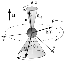
Figure 2: Sketch of the precession angles for the up and down magnetic moments (the arrows depict the directions of their natural precession).

In this case, we assume that the precession angles $\theta_{\sigma}$ (see Fig. 2) of the magnetic moments with $u_{z}>0$ ($\sigma=+1$) and $u_{z}<0$ ($\sigma=-1$) are small, i.e., $\theta_{\sigma}\ll 1$. Then $u_{z}$ can be represented in the form $u_{z}=\sigma(1-\epsilon^{2}/2)$, where according to Eq. (15) a small parameter $\epsilon^{2}$ is given by

$$\epsilon^{2}=\displaystyle\frac{\tilde{h}^{2}}{(\sigma+\tilde{H}-\rho\kappa)^{2}+\lambda^{2}\kappa^{2}},$$ (24)

and so Eq. (14) yields with linear accuracy in $\epsilon$

$$\begin{array}[]{c}u_{x^{\prime}}=\tilde{h}\displaystyle\frac{1+\sigma\tilde{H}-\sigma\rho\kappa}{(\sigma+\tilde{H}-\rho\kappa)^{2}+\lambda^{2}\kappa^{2}},\\[14.0pt] u_{y^{\prime}}=-\tilde{h}\displaystyle\frac{\rho\lambda\kappa}{(\sigma+\tilde{H}-\rho\kappa)^{2}+\lambda^{2}\kappa^{2}}.\end{array}$$ (25)

We emphasize that, even though the static magnetic field is absent, i.e., $\tilde{H}=0$, the dynamics of the up ($\sigma=+1$) and down ($\sigma=-1$) magnetic moments is quite different. The reason is that the natural precession of the magnetic moments is counterclockwise, and so only up or down magnetic moments have the direction of the natural precession that coincides with the direction of the magnetic field rotation. In other words, the magnetic field rotating in the plane perpendicular to the easy axis of magnetization breaks the degeneracy between the up and down states of the magnetic moment.

Our analysis shows that the small-angle precession is stable only if $\tilde{\omega}_{1}+\tilde{\omega}_{4}>0$. Writing $\tilde{\omega}_{1}+\tilde{\omega}_{4}$ with quadratic accuracy in $\epsilon$,

$$\tilde{\omega}_{1}+\tilde{\omega}_{4}=2+2\sigma\tilde{H}-\epsilon^{2}(1-\sigma\tilde{H}+2\sigma\rho\kappa),$$ (26)

and solving the equation $\tilde{\omega}_{1}+\tilde{\omega}_{4}=0$ with respect to $\tilde{H}$, we find the critical magnetic field

$$\tilde{H}_{cr}=-\sigma+\tilde{h}^{2}\frac{\sigma+\rho\kappa}{(1+\lambda^{2})\kappa^{2}}$$ (27)

that separates the stable and unstable precession for a given state $\sigma$. The steady precession is stable either for $\tilde{H}>\tilde{H}_{cr}|_{\sigma=+1}$ or for $\tilde{H}<\tilde{H}_{cr}|_{\sigma=-1}$. Because at $\tilde{H}=\tilde{H}_{cr}$ the precession in the state $-\sigma$ is stable, the switching of the nanoparticle magnetic moments from the unstable state $\sigma$ to the stable state $-\sigma$ occurs. If $\rho=\sigma$, then the rotating field always decreases the stability of the precession, i.e., $\tilde{H}_{cr}|_{\sigma=+1}>-1$ and $\tilde{H}_{cr}|_{\sigma=-1}<+1$. On the contrary, if $\rho=-\sigma$ then depending on the reduced frequency $\kappa$ the rotating field can both decrease (if $\kappa<1$) and increase (if $\kappa>1$) the stability. The largest stabilization effect is achieved at $\kappa=2$. Note also that since $\epsilon\ll 1$ and usually $\lambda<1$, the formula (27) is valid only if the condition $\kappa\gg\tilde{h}$ holds.

As an important illustrative example, we consider the nanoparticle system with the same number $N/2$ of the up and down states. In this case the dynamical (dimensionless) magnetization of the system $\mu_{d}=(1/N)\sum_{i=1}^{N}u_{zi}$ ($i$ labels the nanoparticles) takes the form $\mu_{d}=(1/2)\sum_{\sigma}\sigma\cos\theta_{\sigma}$ or, since $\theta_{\sigma}\ll 1$, $\mu_{d}=(\theta_{-1}^{2}-\theta_{+1}^{2})/4$. Assuming that $\tilde{H}=0$ and using the formula

$$\theta_{\sigma}=\frac{\tilde{h}}{\sqrt{(1-\sigma\rho\kappa)^{2}+\lambda^{2}\kappa^{2}}}$$ (28)

that follows from the relation $\sin\theta_{\sigma}=\epsilon$ and Eq. (24), this quantity can be written in the form

$$\mu_{d}=-\tilde{h}^{2}\frac{\rho\kappa}{[1+(1+\lambda^{2})\kappa^{2}]^{2}-4\kappa^{2}}.$$ (29)

This result shows that (i) the magnetization $\mu_{d}$ is a purely dynamical effect, i.e., $\mu_{d}$ = 0 if $\kappa=\tilde{\omega}/(1+\lambda^{2})=0$, (ii) the direction of magnetization and the direction of magnetic field rotation follow the left-hand rule, and (iii) the dependence of $\mu_{d}$ on $\kappa$ always exhibits a resonant character. The maximum of $\mu_{d}$ occurs at $\kappa=\kappa_{m}$, where

$$\kappa_{m}=\frac{1}{\sqrt{3}(1+\lambda^{2})}\sqrt{1-\lambda^{2}+2\sqrt{1+\lambda^{2}+\lambda^{4}}},$$ (30)

and $\mu_{d}|_{\kappa=\kappa_{m}}=-\rho(\tilde{h}/2\lambda)^{2}$ for $\lambda\ll 1$. If $\tilde{h}\ll\lambda$ then the dynamical magnetization is small but, as we will show later, it can be considerably enhanced by thermal fluctuations.

III.4 Zero static magnetic field

In the case of zero static magnetic field, $\tilde{H}=0$, we rewrite Eq. (15) in the form $\tilde{h}=F_{\rho}(u_{z})$, where

$$F_{\rho}(x)=\frac{\sqrt{1-x^{2}}}{|x|}\sqrt{(x-\rho\kappa)^{2}+(\lambda\kappa x)^{2}}$$ (31)

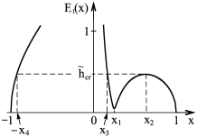
Figure 3: Plot of the function $F_{+1}(x)$ for $\kappa=0.25$ and $\lambda=0.2$. If $\kappa\to 0$, then $x_{n}\to 0$, $F_{+1}(x_{1})\to 0$, and $\tilde{h}_{cr}=F_{+1}(x_{2})\to 1$.

($-1\leq x\leq 1$). According to the definition, the function $F_{\rho}(x)$ satisfies the conditions $F_{\rho}(-x)=F_{-\rho}(x)$, $F_{\rho}(-1)=F_{\rho}(+1)=0$, $F_{\rho}(x)\to\infty$ as $x\to 0$, and it has a local minimum at $x=\rho x_{1}\,(x_{1}>0)$ and a local maximum at $x=\rho x_{2}\,(x_{2}>0)$, see Fig. 3.

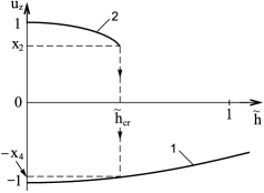
Figure 4: Plots of the stable solutions of the equation $\tilde{h}=F_{+1}(u_{z})$ for the same parameters as in Fig. 3. For $\rho=-1$ the curves 1 and 2 must be reflected with respect to the axis $\tilde{h}$.

A detailed analysis shows that for fixed $\rho$ the precession of the nanoparticle magnetic moment in the state $\sigma=-\rho$ is stable for all values of $\tilde{h}$. In other words, the unique solution of the equation $\tilde{h}=F_{\rho}(u_{z})$ with $\text{sgn}\,u_{z}=-\rho$ always exists and is stable. In this case, the dependence of $u_{z}$ on $\tilde{h}$ is shown in Fig. 4, curve 1.

The precession of the magnetic moment in the state $\sigma=\rho$ (when $\text{sgn}\,u_{z}=\rho$) exhibits qualitatively different behavior depending on $\tilde{h}$. It is stable only if $|u_{z}|>x_{2}$ that implies that $\tilde{h}<\tilde{h}_{cr}=F_{\rho}(\rho x_{2})$ (see Fig. 4, curve 2). At $\tilde{h}=\tilde{h}_{cr}+0$ the solutions $u_{z}|_{\sigma=\rho}=\rho x_{2}$ and $u_{z}|_{\sigma=\rho}=\rho x_{3}\,(x_{3}>0)$ are unstable, and the magnetic moment switches from the state with $u_{z}|_{\sigma=\rho}=\rho x_{2}$ to the new state with $u_{z}|_{\sigma=-\rho}=-\rho x_{4}\,(x_{4}>0)$. As stated above, the new state is stable for all $\tilde{h}$, and so the reverse transition does not occur for fixed $\rho$.

In the important case of small driven frequency, $\kappa\ll 1$, that is easily accessible to experimental investigation, the analysis of the stability of the forced precession can be done analytically. In particular, we found that

$$u_{z}=\sigma\sqrt{1-\tilde{h}^{2}}-\rho\frac{\tilde{h}^{2}}{1-\tilde{h}^{2}}\kappa$$ (32)

if $1-\tilde{h}^{2}\gg\kappa^{2/3}$ and $u_{z}|_{\sigma=-\rho}=-\rho\kappa/\tilde{h}$ if $\tilde{h}\gg 1$. Using the approximate representations

$$\tilde{\omega}_{1}=\tilde{\omega}_{3}=u_{z}^{2}-\rho\frac{\kappa}{u_{z}},\quad\tilde{\omega}_{2}=\tilde{\omega}_{4}=1-\rho\frac{\kappa}{u_{z}},$$ (33)

we showed explicitly that the stability criterion (23) for $\sigma=\rho$ is reduced to $|u_{z}|>x_{2}$ and the critical amplitude of the rotating field is given by $\tilde{h}_{cr}=1-(3/2)\kappa^{2/3}$. Finally, solving the equations $dF_{\rho}(x)/dx=0$ and $\tilde{h}_{cr}=F_{\rho}(x)$ with respect to $x$, we derived the asymptotic formulas $x_{1}=\kappa$, $x_{2}=\kappa^{1/3}$, $x_{3}=\kappa/2$, and $x_{4}=2\kappa^{1/3}$. It is important to note that although the jump $\Delta u_{z}=x_{2}+x_{4}$ that occurs under switching of $u_{z}$ tends to zero as $\kappa\to 0$, it can be sizeable even for very small $\kappa$ (for example, $\Delta u_{z}=0.3$ if $\kappa=10^{-3}$).

We emphasize also that this truly remarkable phenomenon, the switching of the nanoparticle magnetic moments under the action of the rotating field, results from the existence of the natural precession of the magnetic moments. It occurs only in those nanoparticles for which the condition $\sigma\rho=+1$ holds, i.e., if the direction of the magnetic field rotation coincides with the direction of the natural precession of the magnetic moments.

IV THERMAL EFFECTS

IV.1 Mean residence times

If the magnetic moments interact with a heat bath then their dynamics becomes stochastic and is described by the forward Fokker-Planck equation (6). In this case, due to thermal fluctuations, the magnetic moments can perform random transitions from the one state $\sigma$ to the other $-\sigma$. Our aim is to study how the rotating magnetic field influences the mean residence times $t_{\sigma}$ that the magnetic moments dwell in these states at $\tilde{H}=0$. In principle, the problem can be solved on the basis of Eq. (6). Specifically, this approach has been used in the case of ac magnetic field linearly polarized along the easy axis of magnetization.PR However, since the mean residence times can be readily expressed through the mean-first passage times, for solving this problem it is convenient to use the backward Fokker-Planck equationHT ; DY

$$\frac{\partial}{\partial t^{\prime}}P\! = \!-(f_{1}^{\prime}+\gamma^{2}\Delta\cot\theta^{\prime})\frac{\partial}{\partial\theta^{\prime}}P-\gamma^{2}\Delta\frac{\partial^{2}}{\partial\theta^{\prime 2}}P$$ (34)

$$\!-\,f_{2}^{\prime}\frac{\partial}{\partial\varphi^{\prime}}P-\frac{\gamma^{2}\Delta}{\sin^{2}\theta^{\prime}}\frac{\partial^{2}}{\partial\varphi^{\prime 2}}P$$

[$f_{1,2}^{\prime}=f_{1,2}(\theta^{\prime},\varphi^{\prime},t^{\prime})$], which is equivalent to Eq. (6). Within this framework, we are able to calculate $t_{\sigma}$ in some particular cases. But because of the procedure is rather complicated from the mathematical point of view (details will be published elsewhere), here we use a crude approximation that leads, however, to qualitatively the same results.

In the considered case of small-angle precession, the magnetic moments of weakly superparamagnetic particles (when $a=H_{a}m/2k_{B}T\gg 1$) spend almost all time near the conic surfaces with the cone angles (28). We assume that if these imaginary surfaces are replaced by the reflecting surfaces, then the rotating field terms can be eliminated from Eq. (34). Then, replacing also the conditional probability density $P$ by $\bar{P}=\bar{P}(\theta,t|\theta^{\prime},t^{\prime})$ and taking into account that $f_{1}^{\prime}=-(\lambda/2)\omega_{r}\sin 2\theta^{\prime}$, Eq. (34) reduces to the simpler form

$$\frac{\partial}{\partial t^{\prime}}\bar{P}=\bigg{(}\frac{\lambda}{2}\,\omega_{r}\sin 2\theta^{\prime}-\gamma^{2}\Delta\cot\theta^{\prime}\bigg{)}\frac{\partial}{\partial\theta^{\prime}}\bar{P}-\gamma^{2}\Delta\frac{\partial^{2}}{\partial\theta^{\prime 2}}\bar{P}.$$ (35)

Next we use a standard procedure HTB to define the mean first passage times for the magnetic moments in the states $\sigma$

$$T_{\sigma}(\theta^{\prime})=\int_{0}^{\infty}dt\int_{\theta_{\sigma}^{(1)}}^{\theta_{\sigma}^{(2)}}d\theta P(\theta,t|\theta^{\prime},0)$$ (36)

and to derive from Eq. (35) the ordinary differential equation for these quantities

$$\frac{d^{2}T_{\sigma}(\theta^{\prime})}{d\theta^{\prime 2}}+(\cot\theta^{\prime}-a\sin 2\theta^{\prime})\frac{dT_{\sigma}(\theta^{\prime})}{d\theta^{\prime}}+at_{r}=0.$$ (37)

Here, $\theta^{\prime}\in(\theta_{+1},\pi/2)$ if $\sigma=+1$, $\theta^{\prime}\in(\pi/2,\pi-\theta_{-1})$ if $\sigma=-1$, $\theta_{+1}^{(1)}=\theta_{+1}$, $\theta_{+1}^{(2)}=\theta_{-1}^{(1)}=\pi/2$, $\theta_{-1}^{(2)}=\pi-\theta_{-1}$, and $t_{r}=2/\lambda\omega_{r}$ is the characteristic relaxation time of the precessional motion of the magnetic moment. Solving Eq. (37) with the absorbing and reflecting boundary conditions, i.e., $T_{\sigma}(\pi/2)=0$ and $dT_{\sigma}(\theta^{\prime})/d\theta^{\prime}|_{\theta^{\prime}=\pi(1-\sigma)/2+\sigma\theta_{\sigma}}=0$, respectively, and taking into account that the desired times $t_{\sigma}$ are readily expressed through $T_{\sigma}(\theta^{\prime})$, $t_{\sigma}=2T_{\sigma}\textbf{(}\pi[1-\sigma]/2+\sigma\theta_{\sigma}\textbf{)}$, we obtain for $a\gg 1$ and $\theta_{\sigma}\ll 1$

$$t_{\sigma}=\frac{t_{r}}{2}\sqrt{\frac{\pi}{a}}\,\exp[a(1+\sigma 2\tilde{H}_{\sigma})],$$ (38)

where $\tilde{H}_{\sigma}=-\sigma\tilde{\theta}_{\sigma}^{2}/2$ can by interpreted as an effective magnetic field acting on the nanoparticles in the state $\sigma$.

According to this result, the rotating magnetic field decreases the mean residence times. However, due to the natural precession, the decrease of the mean times is different for the up and down magnetic moments. As it will be shown below, this fact causes a strong enhancement of the dynamical magnetization and leads to a modification of the relaxation law.

IV.2 Induced magnetization

We define the steady state magnetization of the nanoparticle system in the rotating magnetic field as $\mu=(1/N)\sum_{i=1}^{N}m_{zi}/m$ ($N\to\infty$). Denoting the average number of the magnetic moments in the state $\sigma$ as $N_{\sigma}$ and introducing the probability $p_{\sigma}=N_{\sigma}/N$ ($p_{+1}+p_{-1}=1$) that the magnetic moment resides in this state, we rewrite $\mu$ in the form

$$\mu=\sum_{\sigma}p_{\sigma}\langle\cos\theta\rangle|_{\sigma},$$ (39)

where $\langle\cos\theta\rangle|_{\sigma}=(1/N_{\sigma})\sum_{i\in N_{\sigma}}\cos\theta_{i}$ is the average value of $m_{zi}/m$ in the state $\sigma$. If $a\gg 1$ then thermal fluctuations are small and $\langle\cos\theta\rangle|_{\sigma}$ in Eq. (39) can be replaced by $\sigma\cos\theta_{\sigma}\approx\sigma(1-\theta_{\sigma}^{2}/2)$, yielding $\mu=\mu_{t}+\mu_{td}+\mu_{d}$. Here $\mu_{t}=\sum_{\sigma}\sigma p_{\sigma}$ and $\mu_{td}=\sum_{\sigma}\sigma(2p_{\sigma}-1)\theta_{\sigma}^{2}/4$ are the contributions of thermal fluctuations to the total magnetization $\mu$, and $\mu_{d}$ is the purely dynamical magnetization given by Eq. (29). Since $\theta_{\sigma}\ll 1$, the condition $\mu_{t}/\mu_{td}\gg 1$ holds, and so $\mu\approx\mu_{t}+\mu_{d}$. We emphasize that a decrease of the temperature (increasing of $a$) decreases the fluctuations of the magnetic moments, but not the difference between $p_{+1}$ and $p_{-1}$, i.e., $\mu_{t}$. Moreover, one expects that, similar to the two-level models, $|\mu_{t}|$ grows with $a$.

Next, taking into account that in the steady state $p_{\sigma}=t_{\sigma}/(t_{+1}+t_{-1})$ and using Eq. (38), we obtain

$$\mu_{t}=\tanh[a(\tilde{H}_{+1}+\tilde{H}_{-1})].$$ (40)

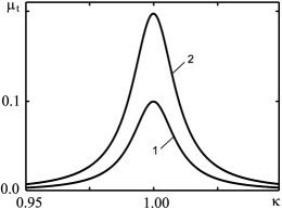
Figure 5: Plots of the magnetization $\mu_{t}$ vs the reduced frequency $\kappa$ for the parameter choice: $\tilde{h}=10^{-3}$, $\lambda=10^{-2}$, $a=20$ (curve 1) and for $a=40$ (curve 2). The temperature in the latter case is two times less than in the former one.

Comparing $\mu_{t}$ with the magnetization of an Ising paramagnet, $\tanh(2a\tilde{H})$, we see that the circularly polarized magnetic field induces the same magnetization $\mu_{t}$ of the nanoparticle system as the external magnetic field $(\tilde{H}_{+1}+\tilde{H}_{-1})/2$ applied perpendicular to the polarization plane. It is interesting to note that $(\tilde{H}_{+1}+\tilde{H}_{-1})/2=\mu_{d}$, and hence $\mu_{t}=\tanh(2a\mu_{d})$. Since $a\gg 1$ and $|\mu_{d}|\ll 1$, this relation shows that $\mu_{t}/\mu_{d}\gg 1$ and so $\mu\approx\mu_{t}$, i.e., thermal fluctuations strongly enhance the dynamical magnetization. In particular, if $a|\mu_{d}|\ll 1$ then $\mu_{t}/\mu_{d}=2a$. Like $\mu_{d}$ the dependence of $\mu_{t}$ on $\kappa$ has a resonant character and, as expected, $|\mu_{t}|$ increases with decreasing temperature (see Fig. 5).

IV.3 Relaxation law

As a second example, let us consider the thermally activated magnetic relaxation in the nanoparticle system driven by the rotating field. Since the transition rate of the nanoparticle magnetic moment from the state $\sigma$ to the state $-\sigma$ equals $1/t_{\sigma}$, the differential equation that defines the time-dependent magnetization $\mu(t)$ of this system can be written in the form

$$\dot{\mu}(t)=-\mu(t)\left(\frac{1}{t_{+1}}+\frac{1}{t_{-1}}\right)-\frac{1}{t_{+1}}+\frac{1}{t_{-1}}.$$ (41)

Assuming that $\mu(0)=1$ (we neglect the dynamical magnetization), from Eq. (41) we obtain the relaxation law

$$\mu(t)=(1-\mu_{t})\exp(-t/\tau)+\mu_{t},$$ (42)

where

$$\tau=\tau_{0}\frac{\exp[a(\tilde{H}_{+1}-\tilde{H}_{-1})]}{\cosh[a(\tilde{H}_{+1}+\tilde{H}_{-1})]}$$ (43)

is the relaxation time in the presence of the rotating magnetic field, and $\tau_{0}=(t_{r}/4)\sqrt{\pi/a}\exp a$ is the relaxation time if the rotating field is absent.

Thus, the rotating magnetic field decreases the relaxation time ($\tau/\tau_{0}<1$) and leads to nonzero magnetization in the long-time limit [$\mu(\infty)=\mu_{t}$].

V CONCLUSIONS

We have investigated a number of dynamical and thermal effects in nanoparticle systems that result from the action of a circularly polarized magnetic field rotating in the plane perpendicular to the easy axes of the nanoparticles. The main finding is that the dynamics of the nanoparticle magnetic moments, both deterministic and stochastic, becomes different in the up and down states. It is important to note that, due to the (counterclockwise) natural precession of the magnetic moments, the dynamics is different even if the static magnetic field is absent.

To describe the dynamical effects at zero temperature, we have used the deterministic Landau-Lifshitz equation. We have solved this equation for small-angle precession of the magnetic moments and have demonstrated that the rotating field, depending on its frequency and polarization, can either decrease or increase the stability of the precession motion. For zero static field, we have calculated the dynamical magnetization of nanoparticle systems and predicted the switching effect. This remarkable effect, which consists in changing the state of the magnetic moments at some critical amplitude of the rotating magnetic field, occurs only for resonant nanoparticles, i.e., when the direction of the natural precession of their magnetic moments coincides with the direction of the magnetic field rotation.

In the case of finite temperatures, we have invoked the backward Fokker-Planck equation to calculate the mean residence times that the driven magnetic moments dwell in the up and down states, respectively. On this basis, we have studied the steady-state magnetization and the features of magnetic relaxation in systems of weakly superparamagnetic nanoparticles that are driven by the rotating magnetic field. In particular, we have found that thermal fluctuations strongly enhance the dynamical magnetization and that the rotating field always causes a decrease of the relaxation time.

Appendix A ROTATING COORDINATE SYSTEMS

A.1 Single-primed coordinate system

The rotating Cartesian coordinate system $x^{\prime}y^{\prime}z^{\prime}$ is defined by the unit vectors $\mathbf{e}_{x^{\prime}}(t)$, $\mathbf{e}_{y^{\prime}}(t)$, and $\mathbf{e}_{z^{\prime}}(t)$ that are expressed through the unit vectors of the initial (laboratory) coordinate system $xyz$ as follows:

$$\begin{array}[]{c}\mathbf{e}_{x^{\prime}}=\cos(\omega t)\mathbf{e}_{x}+\rho\sin(\omega t)\mathbf{e}_{y},\\[12.0pt] \mathbf{e}_{y^{\prime}}=-\rho\sin(\omega t)\mathbf{e}_{x}+\cos(\omega t)\mathbf{e}_{y},\end{array}$$ (44)

$\mathbf{e}_{z^{\prime}}=\mathbf{e}_{z}$. According to Eqs. (44), the inverse transformation has the form

$$\begin{array}[]{c}\mathbf{e}_{x}=\cos(\omega t)\mathbf{e}_{x^{\prime}}-\rho\sin(\omega t)\mathbf{e}_{y^{\prime}},\\[12.0pt] \mathbf{e}_{y}=\rho\sin(\omega t)\mathbf{e}_{x^{\prime}}+\cos(\omega t)\mathbf{e}_{y^{\prime}},\end{array}$$ (45)

and

$$\mathbf{\dot{e}}_{x^{\prime}}=\rho\omega\mathbf{e}_{y^{\prime}},\quad\mathbf{\dot{e}}_{y^{\prime}}=-\rho\omega\mathbf{e}_{x^{\prime}}.$$ (46)

A.2 Double-primed coordinate system

The unit vectors $\mathbf{e}_{x^{\prime\prime}}(t)$, $\mathbf{e}_{y^{\prime\prime}}(t)$, and $\mathbf{e}_{z^{\prime\prime}}(t)$ of the rotating Cartesian coordinate system $x^{\prime\prime}y^{\prime\prime}z^{\prime\prime}$ are introduced as

$$\begin{array}[]{c}\mathbf{e}_{x^{\prime\prime}}=\displaystyle{\frac{(u_{x^{\prime}}\mathbf{e}_{x^{\prime}}+u_{y^{\prime}}\mathbf{e}_{y^{\prime}})u_{z^{\prime}}}{\sqrt{u_{x^{\prime}}^{2}+u_{y^{\prime}}^{2}}}-\sqrt{u_{x^{\prime}}^{2}+u_{y^{\prime}}^{2}}\,\mathbf{e}_{z^{\prime}}},\\[22.0pt] \mathbf{e}_{y^{\prime\prime}}=\displaystyle{\frac{-u_{y^{\prime}}\mathbf{e}_{x^{\prime}}+u_{x^{\prime}}\mathbf{e}_{y^{\prime}}}{\sqrt{u_{x^{\prime}}^{2}+u_{y^{\prime}}^{2}}}},\\[22.0pt] \mathbf{e}_{z^{\prime\prime}}=u_{x^{\prime}}\mathbf{e}_{x^{\prime}}+u_{y^{\prime}}\mathbf{e}_{y^{\prime}}+u_{z^{\prime}}\mathbf{e}_{z^{\prime}},\end{array}$$ (47)

and so the inverse transformation is given by

$$\begin{array}[]{c}\mathbf{e}_{x^{\prime}}=\displaystyle{\frac{u_{x^{\prime}}u_{z^{\prime}}\mathbf{e}_{x^{\prime\prime}}-u_{y^{\prime}}\mathbf{e}_{y^{\prime\prime}}}{\sqrt{u_{x^{\prime}}^{2}+u_{y^{\prime}}^{2}}}+u_{x^{\prime}}\mathbf{e}_{z^{\prime\prime}}},\\[22.0pt] \mathbf{e}_{y^{\prime}}=\displaystyle{\frac{u_{y^{\prime}}u_{z^{\prime}}\mathbf{e}_{x^{\prime\prime}}+u_{x^{\prime}}\mathbf{e}_{y^{\prime\prime}}}{\sqrt{u_{x^{\prime}}^{2}+u_{y^{\prime}}^{2}}}+u_{y^{\prime}}\mathbf{e}_{z^{\prime\prime}}},\\[22.0pt] \mathbf{e}_{z^{\prime}}=-\sqrt{u_{x^{\prime}}^{2}+u_{y^{\prime}}^{2}}\,\mathbf{e}_{x^{\prime\prime}}+u_{z^{\prime}}\mathbf{e}_{z^{\prime\prime}}.\end{array}$$ (48)

From here and (46), straightforward calculations yield

$$\begin{array}[]{c}\mathbf{\dot{e}}_{x^{\prime\prime}}=\rho\omega u_{z^{\prime}}\mathbf{e}_{y^{\prime\prime}},\\[10.0pt] \mathbf{\dot{e}}_{y^{\prime\prime}}=-\rho\omega\left(u_{z^{\prime}}\mathbf{e}_{x^{\prime\prime}}+\sqrt{u_{x^{\prime}}^{2}+u_{y^{\prime}}^{2}}\,\mathbf{e}_{z^{\prime\prime}}\right).\end{array}$$ (49)

References

(1)The Physics of Ultra-High-Density Magnetic Recording, dited by
M. L. Plumer, J. Van Ek, and D. Weller (Springer-Verlag, Berlin, 2001).
(2)
J. L. Dormann, D. Fiorani, and E. Tronc, Adv. Chem. Phys. 98, 283 (1997).
(3)
L. Landau and E. Lifshitz, Phys. Z. Sowjetunion 8, 153 (1935).
(4)
C. H. Back, D. Weller, J. Heidmann, D. Mauri, D. Guarisco, E. L. Garwin, and
H. C. Siegmann, Phys. Rev. Lett. 81, 3251 (1998).
(5)
M. Bauer, J. Fassbender, B. Hillebrands, and R.L. Stamps, Phys. Rev. B 61, 3410 (2000).
(6)
Y. Acremann, C. H. Back, M. Buess, D. Pescia, and V. Pokrovsky, Appl. Phys. Lett. 79, 2228 (2001).
(7)
S. Kaka and S. E. Russek, Appl. Phys. Lett. 80, 2958 (2002).
(8)
H. W. Schumacher, C. Chappert, P. Crozat, R. C. Sousa, P. P. Freitas,
J. Miltat, J. Fassbender, and B. Hillebrands, Phys. Rev. Lett. 90,
017201 (2003).
(9)
Z. Z. Sun and X. R. Wang, Phys. Rev. B 71, 174430 (2005).
(10)
W. F. Brown, Jr., Phys. Rev. 130, 1677 (1963).
(11)
I. Klik and L. Gunther, J. Stat. Phys. 60, 473 (1990).
(12)
W. T. Coffey, D. S. F. Crothers, Yu. P. Kalmykov, E. S. Massawe, and J. T.
Waldron, Phys. Rev. E 49, 1869 (1994).
(13)
D. A. Garanin, Phys. Rev. E 54, 3250 (1996).
(14)
J. L. García-Palacios and F. J. Lázaro, Phys. Rev. B 58, 14937 (1998).
(15)
S. I. Denisov and K. N. Trohidou, Phys. Rev. B 64, 184433 (2001).
(16)
S. I. Denisov, T. V. Lyutyy, and K. N. Trohidou, Phys. Rev. B 67, 014411 (2003).
(17)Nonlinear Phenomena and Chaos in Magnetic Materials, edited by
P. E. Wigen (World Scientific, Singapore, 1994).
(18)
T. Träxler, W. Just, and H. Sauermann, Z. Phys. B 99, 285
(1996).
(19)
G. Bertotti, C. Serpico, and I. D. Mayergoyz, Phys. Rev. Lett. 86,
724 (2001).
(20)
A. F. Khapikov, JETP Lett. 55, 352 (1992).
(21)
A. Magni, G. Bertotti, C. Serpico, and I. D. Mayergoyz, J. Appl. Phys. 89, 7451 (2001).
(22)
S. I. Denisov and A. N. Yunda, Physica B 245, 282 (1998).
(23)
L. S. Pontryagin, Ordinary Differential Equations (Addison-Wesley,
Reading, 1962).
(24)
A. Pérez-Madrid and J. M. Rubí, Phys. Rev. E 51, 4159
(1995).
(25)
P. Hänggi and H. Thomas, Phys. Rep. 88, 207 (1982).
(26)
P. Hänggi, P. Talkner, and M. Borkovec, Rev. Mod. Phys. 62, 251
(1990).