Structure, Scaling and Phase Transition in the Optimal Transport Network

Abstract

We minimize the dissipation rate of an electrical network under a global constraint on the sum of powers of the conductances. We construct the explicit scaling relation between currents and conductances, and show equivalence to a a previous model [J. R. Banavar et al Phys. Rev. Lett. 84, 004745 (2000)] optimizing a power-law cost function in an abstract network. We show the currents derive from a potential, and the scaling of the conductances depends only locally on the currents. A numerical study reveals that the transition in the topology of the optimal network corresponds to a discontinuity in the slope of the power dissipation.

The optimal distribution of valuables such as electricity or telephone signals has been a subject of much study since Westinghouse and Edison’s War of the Currents in the late 19$\rm{}^{t}h$ century ; more recently, natural systems such as river networks and vascular systems have been fruitfully interpreted in this light Rodtiguez-Iturbe and Rinaldo (1997); Rinaldo et al. (1992); Banavar et al. (2000). Hence formal models of optimal transport networks have attracted attention over many years Banavar et al. (1999); Colizza et al. (2004). However, different studies use different definitions of network and optimize different functionals. For example, Durand Durand and Weaire (2004); Durand (2006) considers hydraulic networks whose currents derive from a potential, explicitly analogous to electrical networks; the networks are embedded in an ambient space, and he studies the optimal geometry and the relation between the local geometry and local topology. On the other side, Banavar et al. Banavar et al. (2000) propose a more abstract model where the graph is not assumed to be embedded in a target space, nor are the currents through the nodes explicitly constrained to derive from a potential. This allows them to furnish a strict proof that the topology of the optimized flow pattern Banavar et al. (2000) depends on the convexity of their cost function, but makes a direct physical interpretation of the model more elusive. In the following, we shall introduce a third model of an optimal transport network from whom both of these previous models can be derived, so all formulations are, in fact, equivalent.
Consider an electrical transport network on a graph composed of nodes $k$ interconnected by links $(k,l)$. There is a given current source $i_{k}$ at each node and the total current input must add to zero: $\sum_{k}i_{k}=0$. There are variable currents $I_{kl}$ flowing through the links; the sum of all currents impinging on a given node $k$ must equal the given current sources: $i_{k}=\sum_{l}I_{kl}$ (Kirchhoff’s current law). We associate a resistor $R_{kl}\geq 0$ to each link $(k,l)$ and decompose its value as $R_{kl}=(d_{kl}\kappa_{kl})^{-1}$, where $d_{kl}>0$ is a given weight and the conductances $\kappa_{kl}$ are variable; considering $\kappa_{kl}$ as a conductivity per unit length, $d_{kl}$ can be thought of as the length of the link. The dissipation rate $J$ is then a function of the currents $I_{kl}$ through the links and the conductances $\kappa_{kl}$:

$$J=\sum_{\textrm{links}\,(k,l)}\frac{I_{kl}^{2}}{(d_{kl}\kappa_{kl})}$$ (1)

We shall minimize this dissipation rate $J$ over the currents $I_{kl}$ and the conductances $\kappa_{kl}$ with the local constraint given by Kirchhoff’s current law, and a supplementary global constraint that the sum over the conductances raised to a given power $\gamma>0$ is kept constant:

$$K^{\gamma}=\sum\kappa_{kl}^{\gamma}$$

One may interpret this constant as an amount of resources we have at our disposal to build the network.

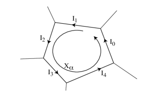
Figure 1: Sketch of a loop $\alpha$ indicating the direction of the currents. Every perturbation of the $I_{kl}$ satisfying the constraints can be written as a weighted sum of such loops.

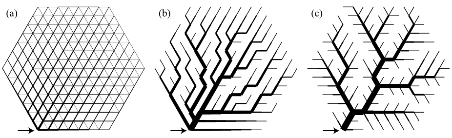
Figure 2: Examples of the conductivity distributions. Results of the relaxation algorithm with different initial conditions: (a) $\gamma=2.0$ and (b) $\gamma=0.5$. (c) Result with optimized topology with $\gamma=0.5$. the arrow indicated the localized inlet, the remaining nodes are outlets with constant $i_{k}$.

Since we allow $\kappa_{kl}$ and $I_{kl}$ to vary independently, the currents are not explicitly constrained to derive from a potential at the nodes $U_{k}$ and Kirchhoff’s voltage law (the sum of the potential differences on a loop vanishes) need not apply.
Using a Lagrange multiplier $\lambda$, we define the function $\Xi(\{\kappa_{kl}\},\{I_{kl}\})$ as

$$\Xi(\{\kappa_{kl}\},\{I_{kl}\})=\sum_{(k,l)}\frac{I_{kl}^{2}}{(d_{kl}\kappa_{kl})}-\lambda\sum_{(k,l)}{\kappa_{kl}}^{\gamma}$$ (2)

The necessary conditions for a minima of $J$ with constant $K$ are then:

$$\frac{\partial\Xi}{\partial I_{kl}}=0,\qquad\frac{\partial\Xi}{\partial\kappa_{kl}}=0$$ (3)

Let us first consider the derivatives with respect to $I_{kl}$. Let $\{\tilde{I}_{kl}\}$, $\{\tilde{\kappa}_{kl}\}$ minimize $J$. Adding a circular current $X_{\alpha}$ on a loop $\alpha$ to the currents (fig. 1) does not violate the constraints. We (re)define the directions of the currents $\tilde{I}_{kl}$ on the loop to be parallel to the loop current $X_{\alpha}$. Then

$$0=\frac{\partial\Xi}{\partial X_{\alpha}}\Big{|}_{X_{\alpha}=0}=\sum_{\textrm{loop}\,\alpha}\tilde{R}_{kl}\tilde{I}_{kl}$$ (4)

Thus Kirchhoff’s voltage law holds at the minimum of $J$, so the currents though the links derive from potential differences between the nodes: $\tilde{I}_{kl}=\tilde{R}_{kl}(U_{l}-U_{k})$. Note that this is not the case for every arbitrary current distribution. For instance, if all currents on the loop in fig. 1 are positive $\tilde{I}_{kl}>0$, then there exists no set of $\tilde{R}_{kl}\geq 0$ to fulfill this relation.
Let us now consider the derivatives of $\Xi$ with respect to $\kappa_{kl}$ (eq. 3). With the constraint of a constant $K$, we obtain an explicit scaling relation between the currents and the conductivity in the minimal configuration:

$$\kappa_{kl}=\frac{(I_{kl}^{2}/d_{kl})^{\frac{1}{1+\gamma}}}{\Big{(}\sum_{mn}{(I_{mn}^{2}/d_{mn})^{\frac{\gamma}{1+\gamma}}}\Big{)}^{1/\gamma}}K$$ (5)

We can now write the total dissipation (eq. 1) in terms of the currents alone as

$${J}(\{I_{kl}\})=\frac{1}{K}\Big{(}\sum_{kl}(I_{kl}^{2}/d_{kl})^{\frac{\gamma}{1+\gamma}}\Big{)}^{1+\frac{1}{\gamma}}$$ (6)

Since for $\gamma>0$, the function $x^{1+\frac{1}{\gamma}}$ is monotonically increasing, the original minimization problem is reduced to the minimization of

$$C(\{I_{kl}\})=\sum_{kl}(I_{kl}^{2}/d_{kl})^{\frac{\gamma}{1+\gamma}}$$ (7)

By setting

$$\Gamma=\frac{2\gamma}{\gamma+1}$$ (8)

and rescaling the weights as $w_{kl}=d_{kl}^{-\frac{\gamma}{1+\gamma}}$, the quantity to be minimized is now

$$C(\{I_{kl}\})=\sum_{kl}w_{kl}\lvert I_{kl}\lvert^{\Gamma}$$ (9)

which is exactly the model used by Banavar et al.Banavar et al. (2000). They give a strict proof that for $\Gamma<1$, the resulting structure may not have any loop, and each spanning tree is a local minimum. For $\Gamma>1$, there are in general loops and a unique minimum. Due to the correspondence between $\gamma$ and $\Gamma$, this result must apply also to our original model where $\gamma<1$ ($\gamma>1$) corresponds to a $\Gamma<1$ ($\Gamma>1$).
On the other hand, the correspondence between the different models allows an important conclusion about the model of Banavar et al.. Since in both formulations, the minimum is obtained by the same set of currents, and since in our model these currents must derive from potential differences between the nodes, this must be true for the minimum of the Banavar et al. model, too. We can furthermore write down directly the values of the corresponding resistors as

$$R_{kl}=(d_{kl}\kappa_{kl})^{-1}=A\,w_{kl}\lvert I_{kl}\rvert^{\Gamma-2}$$ (10)

with an arbitrary positive constant $A$. $R_{kl}$ thus scales explicitly with the local currents for $\Gamma\neq 2$.
Since positive $\gamma$ corresponds to $0<\Gamma<2$, the equivalence of the two models is restricted to this parameter range. $\Gamma>2$ corresponds to values $\gamma<-1$, for which our model collapses into infinitely many degenerate minima. The relations 3 correspond instead to a saddle node of $J$: a minimum with respect to the $I_{kl}$ and a maximum with respect to the $\kappa_{kl}$. Nevertheless direct inspection shows that the current flow in the Banavar et al. model is potential with the set of resistors given by eq. 10 even for $\Gamma>2$.
In order to get a deeper insight into the transition at $\gamma=1$, we search numerically for the minimal dissipation configuration of an example network, a triangular network of conductivities with a hexagonal border, with equal weights $d_{kl}\equiv 1$. The total number of nodes $N_{nodes}$ scales roughly as the square of the linear dimension of the network, given by the diameter of the graph $N_{dia}$. Except for those on the border, each node is linked by conductivities to six neighboring nodes.
We place a current source at a corner of the hexagon ($i_{0}$), the remaining $(N_{nodes}-1)$ nodes present homogeneous distributed sinks; each node absorbs $i_{k}=-i_{0}/(N_{nodes}-1)$.
As an order parameter, we will consider the normalized dissipation rate $J_{min}/J_{homo}$, where $J_{homo}$ is the total dissipation with a constant conductivity distribution $\kappa_{kl}\equiv\textrm{const.}$, and $J_{min}$ is the dissipation for the optimized distribution of the conductivities. Note that $J_{homo}$ corresponds also to $\gamma\rightarrow\infty$.

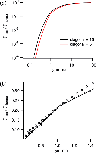
Figure 3: (a) The normalized minimum dissipation rate $J_{min}/J_{homo}$ as a function of $\gamma$ for a network with $N_{dia}=15$ (462 links) and a network with $N_{dia}=31$ (2070 links, in red). Note the discontinuity of the slopes at $\gamma=1$. (b) A detailed view of the crossover at $\gamma=1$ for $N_{dia}=15$. Cross symbols show data points obtained by optimizing a tree topology, circles show the output of the relaxation algorithm. The continuous lines indicate the actual minimum.

The previous discussion allows us to simplify the minimization problem enormously: using the scaling relation between $\kappa_{kl}$ and $I_{kl}$, one can restrict the search of the minimum to the space of the currents or the space of conductivities. Furthermore, we can use the fact that the optimized current distribution derives from a potential $U_{k}$ to construct a simple relaxation algorithm. Starting with a random distribution of $\kappa_{kl}$, we calculate first the values of the potential at the nodes by solving the system of linear equations $i_{k}=\sum_{l}R_{kl}(U_{k}-U_{l})$, then the currents through the links $I_{kl}$ are determined. We use these currents to determine a first approximation of the optimal conductivities on the basis of the scaling relation. Then, the currents are recalculated with this set of conductivities, and the scaling relation is reused for the next approximation. These steps are repeated until the the values have converged. We check by perturbing the solution that it actually is a minimum of the dissipation, which was always the case.
For all $\gamma>1$, independently of the initial conditions, the same conductivity distribution is obtained, which conforms to the analytical result of Banavar et al. (2000): there exists a unique minimum which is therefore global.
Furthermore, the distribution of $\kappa_{kl}$ is “smooth”, varying only on a “macroscopic scale”, as show in Fig. 2(a)). No formation of any particular structure occurs. However, the conductivity distribution is not isotropic. We can interpret the conductivity distribution as a discrete approximation of a continuous, macroscopic conductivity tensor (see also Durand and Weaire (2004)). The smooth aspect of the distribution is conserved while approaching $\gamma\rightarrow 1$ while the local anisotropy increases, while the values of all $\kappa_{kl}$ remain finite, even if they get very small. For $\gamma=1.5$ and $N_{dia}=15$, the conductivity distribution spreads already over eight decades and becomes still broader as $\gamma\rightarrow 1^{+}$, in which limit the number of iteration steps diverges as the minima becomes less and less steep.
$\gamma=1$ presents a marginal case. The results of the simulation suggest that the minimum is highly degenerate, i.e., there are a large number of conductivity distributions yielding the same minimal dissipation.
For $\gamma<1$, the output of the relaxation algorithm is qualitatively different (fig. 2(b)). The currents are canalized in a hierarchical manner: a large number of conductivities rapidly converge to zero and thus vanish transforming the topology from a highly redundant network to a spanning tree. This, too, is predicted by the analytical results Banavar et al. (2000). In contrast to $\gamma>1$, the conductivity distribution can not be interpreted as a discrete approximation of a conductivity tensor: for $N_{dia}\rightarrow\infty$, the structure becomes fractal.
For different initial conditions, the relaxation algorithm yields trees with different topologies: each local minima in the high-dimensional and continuous space of conductivities $\{\kappa_{kl}\}$ correspond to a different tree topology. Given a tree topology, the currents through the links are given directly by the topology and do not depend on the values of the $\kappa_{kl}$, and so using the scaling relation, one may directly write down the dissipation rate for a given tree. For $\gamma<1$, we do thus not need to apply the relaxation algorithm, but we should search for the global minima in the (exponentially large) space of tree topologies using a Monte-Carlo algorithm. This regime has been widely explored in the context of river networks Rinaldo et al. (1992); Sun et al. (1994); Rodtiguez-Iturbe and Rinaldo (1997), mainly for a set of parameters that corresponds, in our case, to $\gamma=0.5$. An example of a resulting minimal dissipation tree structure is given in fig. 2(c). Note also, that the scaling relations can be seen as some kind of erosion model: the more currents flows trough a link, the better the link conducts Rodtiguez-Iturbe and Rinaldo (1997).
The qualitative transition is reflected also quantitatively in the value of the minimal dissipation (fig 3(a)). The points for $\gamma>1$ were obtained with the relaxation algorithm, the points $\gamma<1$ by optimizing the tree topologies with a Monte-Carlo algorithm. For $\gamma\rightarrow\infty$, $J_{min}/J_{homo}\rightarrow 1$ by definition; for $\gamma\rightarrow 0$, $J_{min}/J_{homo}\rightarrow 0$, because the vanishing $\kappa_{kl}$ allow the the remaining $\kappa_{kl}\rightarrow\infty$.
Figure 3(b) shows the behavior of minimal dissipation rate close to $\gamma=1$. For $\gamma$ smaller than one, the relaxation method spends a long time only to furnish a local minimum, while the Monte-Carlo algorithm searching for the optimal tree topologies gives lower dissipation values. The different values corresponding to different realization indicate that the employed Monte-Carlo method does not find the exact global minima. For $\gamma>1$, the relaxation algorithm gives the lower $J_{min}$ because the global minima does not have a tree topology.
While the curve is continuous, the crossover at $\gamma=1$ shows a clear change in the slope of $J_{min}(\gamma)$. One could interpret this behavior as a second order phase transition. (The change in slope is of course preserved in the function $C({I_{kl}})$ used by Banavar et al. (2000).)
As an intriguing practical application of these models, one may for instance cite the venation of plant leaves. Experimental evidence Zwieniecki et al. (2002) shows that the water transport through the veins derives from a pressure gradient. The venation pattern however shows a enormous redundancy of loops Esau (1953); Roth-Nebelsick et al. (2001); Couder et al. (2002). On the basis of some examples, it has been proposed Roth et al. (1995); Roth-Nebelsick et al. (2001) that the loops are actually meaningful to optimize the water transport in the leaf. The results presented in this paper however shows that this is not the case: optimization either leads to a tree topology, or to no structure at all. If the venation pattern is really based a optimization principe, it cannot simply be optimization of a steady state water transport, even if Murray’s law seems to hold at the nodes of the venation McCulloh et al. (2003).

References

- Rodtiguez-Iturbe and Rinaldo (1997) I. Rodtiguez-Iturbe and A. Rinaldo, Fractal River Basins (Cambrige University Press, Cambrige, New York, 1997).
- Rinaldo et al. (1992) A. Rinaldo, I. Rodriguez-Iturbe, R. Rigon, R. Bras, E. Ijj sz-V squez, and A. Marani, Water Resour. Res. 28, 2183 (1992).
- Banavar et al. (2000) J. R. Banavar, F. Colaiori, A. Flammini, A. Maritan, and A. Rinaldo, Phys. Rev. Lett. 84, 004745 (2000).
- Banavar et al. (1999) J. R. Banavar, A. Maritan, and A. Rinaldo, Nature 399, 130 (1999).
- Colizza et al. (2004) V. Colizza, J. Banavar, A. Maritan, and A. Rinaldo, Phys. Rev. Lett. 92, 198701 (2004).
- Durand and Weaire (2004) M. Durand and D. Weaire, Phys. Rev E 70, 046125 (2004).
- Durand (2006) M. Durand, Phys. Rev E 73, 016116 (2006).
- Sun et al. (1994) T. Sun, P. Meakin, and T. Jossag, Phys. Rev. E 49, 4865 (1994).
- Zwieniecki et al. (2002) M. Zwieniecki, P. Mecher, C. Boyce, L. Sack, and N. Holbrook, Plant, Cell and Environmenmt 25, 1445 (2002).
- Esau (1953) K. Esau, Plant anatomy (Wiley, 1953).
- Roth-Nebelsick et al. (2001) A. Roth-Nebelsick, D. Uhl, V. Mosburgger, and H. Kerp, Annals of Botany 87, 553 (2001).
- Couder et al. (2002) Y. Couder, L. Pauchard, C. Allain, M. Adda-Bedia, and S. Douady, Eur. Phys. J. B 28, 135 (2002).
- Roth et al. (1995) A. Roth, V. Mosbrugger, H. Neugebauer, and G. Belz, Botanica Acta 108, 121 (1995).
- McCulloh et al. (2003) K. McCulloh, J. Sperry, and F. Adler, Nature 421, 939 (2003).