Kondo effect with non collinear polarized leads:
a numerical renormalization group analysis

Abstract

The Kondo effect in quantum dots attached to ferromagnetic leads with general polarization directions is studied combining poor man scaling and Wilson’s numerical renormalization group methods. We show that polarized electrodes will lead in general to a splitting of the Kondo resonance in the quantum dot density of states except for a small range of angles close to the antiparallel case. We also show that an external magnetic field is able to compensate this splitting and restore the unitary limit. Finally, we study the electronic transport through the device in various limiting cases.

I Introduction

One of the most remarkable achievements of recent progress in nanoelectronics has been the observation of the Kondo effect in a single semiconductor quantum dot (QD).dot ; Cronenwett Since these early experiments, the Kondo effect has also been observed in carbon nanotube QDs,cobden ; bachtold ; jarillo and molecular transistorsmolecular connected to normal metallic leads. The success of these experiments has opened the way to a systematic analysis, both theoretically and experimentally, of the effects of the leads correlations on the Kondo effect. Of particular interest are the experimental realizations of the Kondo effect connected to superconducting leadssupra or to ferromagnetic electrodes.ralph The latter is particularly important since it is connected to the new emerging field called “spintronics”.loss One goal of spintronics is to provide devices where the transport properties are controlled by magnetic degrees of freedom. In this sense, a Kondo quantum dot connected to ferromagnetic electrodes may be regarded as an interesting setup to study interaction effects in spintronics devices.

From the theoretical point of view, it has been predicted, despite some early controversial results,sergueev ; zhang ; bulka ; lopez1 that ferromagnetic electrodes with parallel polarization produce a splitting of the Kondo zero bias anomalymartinek1 ; martinek2 ; lopez2 whereas polarized electrodes with antiparallel polarization generally do not.martinek1 ; lopez2 ; utsumi Some of these predictions have been checked experimentally by contacting C₆₀ molecules with ferromagnetic nickel electrodes. ralph The underlying mechanism responsible of the splitting of the Kondo resonance is quite clear: virtual quantum charge fluctuations between the dot and the leads become spin dependent. As a result, an effective exchange magnetic field appears in the dot which generally lifts the spin degeneracy on it. For antiparallel configurations, the contributions of each electrode to the effective field may eventually cancel each other for symmetric couplings.

Most of the previous works have focused quite surprisingly only on parallel and antiparallel polarizations. Sergueev et al. sergueev considered non collinear polarizations but did not take into account the spin splitting of the dot energy level which naturally gives rise to spurious results. In a recent preprint, Swirkowicz et al.barnas analyze the non collinear situation using the equation of motion method supplemented by an effective exchange field that has to be determined self-consistently. Such method gives qualitative results for temperature $T\sim T_{K}$, where $T_{K}$ is the Kondo temperature. The main result is that the splitting of the zero bias Kondo anomaly decreases monotonically when increasing the angle $2\theta$ between the two lead magnetizations. In this paper, we go beyond the equation of motion method by combining a poor man scaling approach and the numerical renormalization group (NRG) approach. The poor man scaling provides us with an analytical expression for the Kondo temperature as a function of the lead polarization $p$ and $\theta$ [see Eq.(12)] while NRG allows us to compute dot spectral densities and the near equilibrium transport properties like the conductance. The plan of the paper is the following: In Sec. II we describe our model Hamiltonian. In Sec. III, we use poor man scaling to estimate the Kondo temperature. In Sec. IV, we present the NRG results for the dot density of states and for the conductance. Finally, Sec. V contains a brief summary of the results.

II Model Hamiltonian

In order to describe this system we use the following general Hamiltonian

$$H=H_{leads}+H_{tun}+H_{dot},$$ (1)

where $H_{leads}$ denotes the Hamiltonian of the conduction electrons in the leads and is defined by

$$H_{\mathrm{leads}}=\sum\limits_{k,\gamma,\pm}\varepsilon_{k\pm}c_{k,\gamma,\pm}^{{\dagger}}c_{k,\gamma,\pm}.$$ (2)

In this equation $c_{k,\gamma,\pm}^{{\dagger}}$ creates an electron with energy $\varepsilon_{k\pm}$ in lead $\gamma=L,R$ with spin along $\pm\vec{n}_{\gamma}$ where $\vec{n}_{\gamma}$ is a unitary vector parallel to the magnetization moment in lead $\gamma$. The angle between $\vec{n}_{L}$ and $\vec{n}_{R}$ is $2\theta$. Since the leads are assumed to be polarized, there is a strong spin asymmetry in the density of states $\rho_{\gamma\pm}(\omega)$. The tunneling junctions between the leads and the dot may be described by a standard tunneling Hamiltonian

$$H_{tun}=\sum\limits_{k,\gamma,\sigma=\uparrow,\downarrow}(t_{\gamma}c_{k,\gamma,\sigma}^{{\dagger}}d_{\sigma}+H.c.),$$ (3)

where $d_{\sigma}$ destroys an electron in the dot with spin $\sigma=\uparrow,\downarrow$. Here the possible values for the dot spin are quantized along the axis $\vec{e}_{z}=(\vec{n}_{L}+\vec{n}_{R})/|\vec{n}_{L}+\vec{n}_{R}|$. The operator $c_{k,\gamma,\sigma}$ is a linear combination of the operators $c_{k,\gamma,s=\pm}$ and reads:

$$\left(\begin{array}[]{c}c_{\alpha,k,\uparrow}\\ c_{\alpha,k,\downarrow}\end{array}\right)=\left(\begin{array}[]{cc}\cos(\frac{\theta_{\alpha}}{2})&-\sin(\frac{\theta_{\alpha}}{2})\\ \sin(\frac{\theta_{\alpha}}{2})&\cos(\frac{\theta_{\alpha}}{2})\end{array}\right)\left(\begin{array}[]{c}c_{\alpha,k,+}\\ c_{\alpha,k,-}\end{array}\right),$$ (4)

where $\theta_{\alpha}=\pm\theta$ here. $H_{dot}$ is the usual Anderson Hamiltonian and reads

$$H_{dot}=\sum_{\sigma=\uparrow,\downarrow}\varepsilon_{d,\sigma}d_{s}^{{\dagger}}d_{s}+Ud_{\uparrow}^{{\dagger}}d_{\uparrow}d_{\downarrow}^{{\dagger}}d_{\downarrow}-g\mu_{B}BS^{z},$$ (5)

where $S^{z}=(d_{\uparrow}^{{\dagger}}d_{\uparrow}-d_{\downarrow}^{{\dagger}}d_{\downarrow})$. The last term of Eq. (5) describes the Zeeman energy splitting of the dot. In what follows we mainly consider a symmetric situation in which $t_{\gamma}=t$. We denote the total tunneling strength by $\Gamma=\Gamma_{L}+\Gamma_{R}$ with $\Gamma_{L}=\pi t^{2}(\rho_{+}+\rho_{-})$. The effective magnetic fields generated by the ferromagnetic electrodes is then along the axis $\vec{e}_{z}=(\vec{n}_{L}+\vec{n}_{R})/|\vec{n}_{L}+\vec{n}_{R}|$. We next perform a poor man scaling analysis.

III Poor man scaling analysis

The analysis extends in a straightforward manner the one developed in Ref. [martinek1, ]. In this part we neglect the energy dependence in the density of states and also suppose $\rho_{\gamma\pm}\approx\rho_{\pm}$. In the ferromagnetic leads, the ratio $p=(\rho_{+}-\rho_{-})/(\rho_{+}+\rho_{-})$ is in general different from zero and as shown bellow it is one of the relevant parameters to describe the effect of the spin polarization. For an energy dependent density of states, the situation is more complex as will be shown in Sec. IV. One performs a two stage renormalization group (RG) analysis by reducing the cutoff $\Lambda$ from $D$ the bandwidth to $\bar{\varepsilon}_{d}=\varepsilon_{d\uparrow}+\varepsilon_{d\downarrow}$ which renormalizes the parameters of the Anderson model. In general, $\varepsilon_{\uparrow}$ and $\varepsilon_{\downarrow}$ renormalize differently due to the spin dependent density of states (DOS) in the leads.martinek1 The spin degeneracy of the Anderson energy levels is therefore lifted with an effective Zeeman splitting

$$\delta\varepsilon_{d}=\varepsilon_{d\uparrow}-\varepsilon_{d\downarrow}\sim p\Gamma\cos(\theta)\ln(D/\Lambda).$$ (6)

This splitting prevents from reaching of the strong coupling regime. Nonetheless, an external magnetic field $B$ can be applied locally to compensate this internal field and restore the degeneracy between $\varepsilon_{\uparrow}$ and $\varepsilon_{\downarrow}$. One can then perform a Schrieffer-Wolff transformation. The Kondo Hamiltonian so obtained is similar to the usual Kondo Hamiltonian:

$$H_{K} = \frac{1}{2}\sum\limits_{k,k^{\prime},\alpha,\beta}(J^{z\uparrow}c_{k\alpha\uparrow}^{{\dagger}}c_{k\beta\uparrow}-J^{z\downarrow}c_{k\alpha\downarrow}^{{\dagger}}c_{k\beta\downarrow})S^{z}$$ (7)

$$+ J^{\perp}(c_{k\alpha\downarrow}^{{\dagger}}c_{k\beta\uparrow}S^{+}+c_{k\alpha\uparrow}^{{\dagger}}c_{k\beta\downarrow}S^{-}).$$

The bare values of the Kondo couplings are

$$J^{\perp}=J^{z\uparrow}=J^{z\downarrow}\sim 2t^{2}\left(\frac{U}{(|\varepsilon_{d}|(\varepsilon_{d}+U)}\right)=J,$$ (8)

where $\varepsilon_{d}\sim\varepsilon_{d\uparrow}\sim\varepsilon_{d\downarrow}$. Note also that $\psi_{L\uparrow}$ is a linear superposition of $\psi_{L+}$ and $\psi_{L-}$. One can then perform the second stage of the RG analysis directly on the Kondo Hamiltonian. The RG equations can be obtained by integrating out the high energy degrees of freedom between a cut-off $\Lambda_{0}\sim{\varepsilon}_{d}$ and $\Lambda$ and read:

$$\frac{d\lambda_{z\uparrow}}{d\ln l} = 2\left[\cos^{2}(\theta/2)+\frac{1+p}{1-p}\sin^{2}(\theta/2)\right]\lambda_{\perp}^{2},$$ (9)

$$\frac{d\lambda_{z\downarrow}}{d\ln l} = 2\left[\cos^{2}(\theta/2)+\frac{1-p}{1+p}\sin^{2}(\theta/2)\right]\lambda_{\perp}^{2},$$ (10)

$$\frac{d\lambda_{\perp}}{d\ln l} = \left[\cos^{2}(\theta/2)+\frac{1-p}{1+p}\sin^{2}(\theta/2)\right]\lambda_{\perp}\lambda_{z\uparrow}$$ (11)

$$+ \left[\cos^{2}(\theta/2)+\frac{1+p}{1-p}\sin^{2}(\theta/2)\right]\lambda_{\perp}\lambda_{z\downarrow},$$

where we have introduced the dimensionless Kondo couplings $\lambda_{\perp}=\sqrt{\rho_{+}\rho_{-}}J^{\perp}$, $\lambda_{z\uparrow/\downarrow}=\rho_{\pm}J^{z,\uparrow/\downarrow}$ and $l=\Lambda_{0}/\Lambda$. The dimensionless Kondo couplings are all driven to strong coupling at the same energy scale $T_{K}$ which can be determined explicitly by integrating out the above RG equations. The Kondo temperature can be expressed as:

$$T_{K}(p,\theta)=\Lambda_{0}\exp\left(-\frac{\mathrm{arctanh}(p\cos(\theta))}{2\lambda_{0}p\cos(\theta)}\right),$$ (12)

where $\lambda_{0}=J_{0}(\rho_{+}+\rho_{-})$. This expression generalizes the one obtained in Ref. [martinek1, ] to all values of $\theta$. The dependence of the Kondo temperature with $p,\theta$ appears as a function of the single parameter $p\cos(\theta)$ and is therefore a uniform function of $\theta$. $T_{K}$ takes its maximum value $T_{K}^{0}$ independent of $p$ at $\theta=\pi/2$ which corresponds to antiparallel magnetizations and $T_{K}$ is minimum for $\theta=0$ as expected.

IV Numerical renormalization group analysis

In order to compute dot spectral densities and transport properties we proceed with a NRG analysis. At this point it is convenient to perform two unitary transformations on the initial Hamiltonian defined in Eq. (1). We first make an even/odd transformation introducing the operators

$$c_{k,e/o,\pm}=(c_{k,L,\pm}\pm c_{k,R,\pm})/\sqrt{2}.$$ (13)

We next introduce a new basis defined by

$$b_{k,e,\uparrow/\downarrow}=c_{k,e,\pm}~{}~{},~{}~{}b_{k,o,\uparrow/\downarrow}=c_{k,e,\mp}.$$ (14)

The tunneling Hamiltonian can be written in the new basis as:

$$H_{tun}=\sum\limits_{k,\eta=e/o,\sigma}(t_{\eta}b^{\dagger}_{k\eta,\sigma}d_{\sigma}+H.c.)$$ (15)

where $t_{e}=t\sqrt{2}\cos(\theta/2)$, and $t_{o}=t\sqrt{2}\sin(\theta/2)$. The crucial point is that the angle $\theta$ arising due to the non collinear lead magnetizations is now hidden in the tunneling amplitudes $t_{e}$ and $t_{o}$.

Note that in this formulation the dot is coupled with a single effective lead with an angle and spin dependent bulk spin DOS given by

$$\rho^{eff}_{\uparrow/\downarrow}=\rho_{\pm}\cos^{2}(\theta/2)+\rho_{\mp}\sin^{2}(\theta/2),$$ (16)

which is mixture of the initial bulk spin densities of states. This allows us to treat this problem in a simplified way using the numerical renormalization group method hewson-book ; hofstetter ; costi with the generalizations to treat arbitrarily shaped densities of states. ingersent

We insist that such formulation has been made possible only because we consider symmetric tunneling amplitudes $t_{L}=t_{R}$. Note that for antiparallel polarizations ($\theta=\pi/2$) we have $\rho^{eff}_{\uparrow}=\rho^{eff}_{\downarrow}$ and the effective model has spin symmetry.

IV.1 Study of the dot density of states

From hereon we will consider the DOS along the polarization direction in each lead to be given by the tight-binding expressions

$$\rho_{\pm}(\omega)=\frac{2}{\pi D}\sqrt{1-\left(\frac{\omega+\delta\epsilon_{\pm}}{D}\right)^{2}},$$ (17)

where $\delta\epsilon_{+}=-\delta\epsilon_{-}=\delta\epsilon$ is the spin-dependent shift of the bands with respect to the Fermi level. The quantity $\delta\epsilon$ characterizes the magnetization $P$ of the leads given by

$$P=\int_{-\infty}^{\infty}d\omega f(\omega)[\rho_{+}(\omega)-\rho_{-}(\omega)],$$ (18)

where $f(\omega)$ is the Fermi function. Note that the densities of states in the leads are no longer constant which is more realistic to describe ferromagnetic leads. konig04 For the sake of simplicity, from hereon we take the chemical potential equal to zero. Note that for this particular choice the parameter $p$ defined in the previous section is zero while the spin polarization is not. For small $\delta\epsilon$ and temperatures the magnetization is simply given by $P\simeq\frac{4\delta\epsilon}{\pi D}$. In the present case, the most important effect of the leads magnetism is the occurrence of an internal field $B_{int}$ that creates the effective Zeeman splitting already mentioned above.

To calculate the dot density of states we need the local Green function. In the standard form, we have

$$G^{-1}_{\sigma}{(\omega{})}=G^{-1}_{0\sigma}(\omega)-\Sigma(\omega),$$ (19)

where $\Sigma_{\sigma}(\omega)$ is the self-energy and $G_{0\sigma}(\omega)^{-1}$ is the non-interacting Green function

$$G_{0\sigma}(\omega)=\frac{1}{\omega-\epsilon_{d,\sigma}-g\mu B\sigma-\Delta_{\sigma}(\omega)}.$$ (20)

The hybridization function $\Delta_{\sigma}(\omega)$ is spin-dependent and has in general a non-zero real part that is given by

$${\cal R}[\Delta_{\sigma}(0)]=\sigma 4t^{2}\delta\epsilon\cos(\theta)/D^{2},$$ (21)

for our choice of the DOS and $\omega\sim 0$. This is equivalent to an angle-dependent effective magnetic field

$$\mu_{B}B_{int}=8t^{2}\delta\epsilon\cos(\theta)/D^{2},$$ (22)

that polarizes the dot’s spin and destroys the Kondo effect for $\mu_{B}B_{int}\gtrsim T_{K}$.

The first thing we want to check is whether the polarized leads with a given angle $\theta$ are able to split the dot DOS [$\rho_{\sigma}(\omega)=-{\cal I}[G_{\sigma}(\omega)]/\pi$]. It has been shown that polarized leads with antiparallel polarized directions (corresponding to $\theta=\pi/2$ here) do not split the dot density of states.lopez1 ; martinek1 Is there a finite interval around $\theta=\pi/2$ where this property holds? We have plotted in Fig. 1 the dot spectral density $\rho_{\uparrow}$ in the spin up sector for different values of $\theta$. As expected the low energy peak of $\rho_{\uparrow}$ is pinned at $\omega=0$ for $\theta=0$ but is shifted away from $\omega=0$ as soon as $\theta$ is decreased. This is much clearer in the right inset of Fig. 1 where the peak is zoomed.

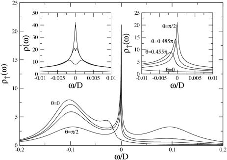
Figure 1: Dot density of states for the spin-up sector as function of energy for different values of $\theta=0,\,0.455\pi,\,0.485\pi,\,\pi/2$. The shift of the bands is fixed to $\delta\epsilon=0.5D$. Other parameter are: $U=0.2$, $\epsilon{{}_{d}=-U/2}$, and $t=0.071$. Right inset: zoom of $\rho_{\uparrow}$ for the same values of $\theta$. We clearly see the shift of the maximum $\rho_{\uparrow}$ when decreasing $\theta$ away from $\theta=\pi/2$. Left inset: Total density of states as function of frequency for the four aforementioned values of $\theta$. The density of states is split as soon as the effective magnetic field is larger than the Kondo temperature.

The splitting of the total dot density of states $\rho=\rho_{\uparrow}+\rho_{\downarrow}$ is shown in the left inset of Fig. 1 for four different values of $\theta$. The splitting gradually increase as $\theta$ is decreased from $\theta=\pi/2$ and is maximum for $\theta=0$. For very small deviations of $\theta$ around $\pi/2$, the effective magnetic field $\mu_{B}B_{int}\lesssim T_{K}$ and no splitting is expected.

For collinear polarization directions, it has been shown that this splitting can be compensated by an external magnetic field martinek2 restoring the Kondo effect. For general directions of the lead polarizations, an effective magnetic field is also generated. This effective magnetic field can be compensated by applying an external magnetic field in the plane $(\vec{n}_{L},\vec{n}_{R})$ with a direction opposite to $\vec{e}_{z}$. We therefore expect that the splitting of the Kondo zero bias anomaly induced by the polarized electrodes can be corrected by an adequate magnetic field for all values of $\theta$. We have checked that this property holds using NRG. We have presented in Fig. 2 the DOS $\rho_{\uparrow}$ as function of energy for $\theta=0$ (where the splitting is maximum) and for different value of the external magnetic field. For a given value of the external magnetic field, the splitting of the Kondo peak vanishes and the Kondo peak is restored at $\omega=0$. This is also true for a general angle $\theta$ (see Fig. 3). These properties of the dot’s spectral density will clearly reflect in the transport properties of the system as we will see.

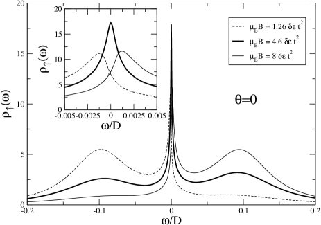
Figure 2: Dot density of states for the spin-up sector as function of energy for different values of the magnetic field in the case with parallel magnetizations ($\theta=0$). Other parameters as in Fig. 1. The spin polarization in the dot and the splitting of the Kondo peak can be compensated with a magnetic field.

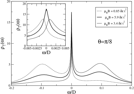
Figure 3: Same as Fig. 2 with $\theta=\pi/8$.

IV.2 Transport properties

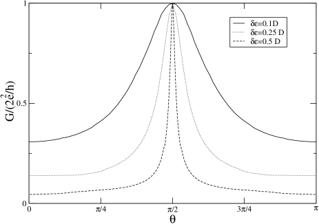
Figure 4: Conductance as a function of the angle for different values of the bands shift $\delta\epsilon=0.1D,\,0.25D,\,0.5D$. Other parameters as in Fig. 1.

Using the Keldysh formalism, it has been shown that for the collinear magnetizations, as in the case of non-magnetic leads, the finite temperature conductance can be put in terms on the dot’s spectral density. mw This is not the case for arbitrary angles. The problem is that for non collinear magnetizations, the two spin channel of the $L$ and $R$ leads are mixed and the standard approach used to eliminate the lesser propagator can not be applied. To our knowledge, in these circumstances, the only direct way of evaluating the conductance at any temperature is through the Kubo formalism. This requires evaluating two particle propagators, a matter that requires sophisticated numerical codes. There are however some limiting cases that illustrate the general behavior as we will see. In our NRG formulation we have $\rho_{d\uparrow}(0)=\rho_{d\downarrow}(0)$. Since the DOS in the leads are energy dependent (see Eq. (17)), this equality does not prevent to have a non zero polarization following Eq. (18) though $p=0$. For this case, the hybridization matrices $\Gamma_{\sigma\sigma^{\prime}}=-{\cal I}(\Sigma_{\sigma\sigma^{\prime}})$ (where $\sigma,\sigma^{\prime}=\uparrow,\downarrow$) are diagonal and angle independent. This allows the use of the Meir Wingreen formula. mw The $T=0$ conductance is thus simply proportional to $|G_{d}(0)|^{2}$. The $T=0$ conductance has been computed using NRG and is shown in Fig. 4 as a function of $\theta$ for different values of the splitting $\delta\varepsilon$. The conductance reaches the unitary limit for $\theta=\pi/2$ (antiparallel case) and is minimum for parallel magnetizations. Though this result may look unusual, this is expected since the splitting is zero for $\theta=\pi/2$ restoring the Kondo effect and is maximum for $\theta=0$. Remember that $p(0)=0$ with the definition of the DOS we used in NRG.

This result should be contrasted to the situation where an external magnetic field able to restore the Kondo zero bias anomaly is added. We consider constant bulk DOS as in Sec. III. Electrons with spins $\uparrow$ have a different DOS at the Fermi energy than electrons with spins $\downarrow$, resulting in $p(0)\neq 0$ (as in [lopez1, ; martinek1, ; martinek2, ]). At $T=0$, the Kondo singlet is therefore formed and the Fermi liquid theory can be applied. The conductance $G$ through the device reaches at $T=0$ its maximum conductance $G_{u}$ which reads:

$$G_{u}=\frac{2e^{2}}{h}\frac{1-p^{2}}{1-p^{2}\cos^{2}(\theta)}~{}.$$ (23)

Notice that here $G$ reaches the unitary limit for $\theta=0$ whatever the value of $p$ and is minimum for $\theta=\pi/2$ at fixed $p$. In order to determine to determine $G_{u}$, we have extended the scattering approach developed by Ng and Lee ng to polarized electrodes following [martinek2, ]. This anomalous denominator comes from the fact the imaginary part of the dot retarded Green function $G_{d\sigma}^{r}$ is simply $-1/\Gamma_{\sigma\sigma}$ at $T=0$ which depends on the angle $\theta$ and $p$. At finite $T\ll T_{K}(p,\theta)$, deviations of order $(T/T_{K})^{2}$ from $G_{u}$ are expected using the Fermi liquid theory. On the other hand, at high temperature $T\gg T_{K}(p,\theta)$, the conductance is much smaller and can be computed by renormalized perturbation theory:

$$G=\frac{2e^{2}}{h}(1+p^{2}\cos(2\theta))\frac{3\pi^{2}/16}{\ln^{2}(T/T_{K})}.$$ (24)

Notice that the expression for the high temperature conductance has the same angular expression as the one for a tunnel junction between two ferromagnetic leads conversely to the low temperature case.

V Conclusion

In this paper, we have studied a quantum dot in the Kondo regime between two non collinear ferromagnetic electrodes by combining poor man scaling and NRG techniques. We have shown using NRG that the Kondo zero bias anomaly is in general splitted for all angles between the two lead magnetizations (except for the antiparallel case). This splitting can be compensated by an external magnetic field. Based on the spectral densities, we have addressed transport properties for both compensated and uncompensated cases.

Note added Some of the results presented in this paper have been also independently obtained in a recent preprint eto . Acknowledgments. – PS would like to thank interesting communications with J. Martinek. Part of this research was supported by the contract PNANO ‘QuSpins’ of the French Agence Nationale de la Recherche.

References

- (1) D. Goldhaber-Gordon, H. Shtrikman, D. Mahalu, D. Abusch-Magder, U. Meirav, and M.A. Kaster, Nature 391, 156 (1998).
- (2) S. M. Cronenwett, T.H. Oosterkamp, and L.P. Kouwenhoven, Science 281 , 540 (1998); F. Simmel, R. H. Blick, U.P. Kotthaus, W. Wegsheider, and M. Blichler, Phys. Rev. Lett. 83, 804 (1999); J. Schmid, J. Weis, K. Eberl, and K. v. Klitzing, Phys. Rev. Lett. 84, 5824 (2000); W. G. van der Wiel, S. De Franceschi, T. Fujisawa, J.M. Elzerman, S. Tarucha, and L. P. Kouwenhoven, Science 289, 2105 (2000).
- (3) J. Nygård, H. Cobden, and P. E. Lindelof, Nature 408, 342 (2000).
- (4) M. R. Buitelaar, A. Bachtold, T. Nussbaumer, M. Iqbal, and C. Schönenberger, Phys. Rev. Lett. 88, 156801 (2002).
- (5) P. Jarillo-Herrero, J. Kong, H. S. J. van der Zant, C. Dekker, L. P. Kouwenhoven, and S. De Franceschi, Nature 434, 484 (2005).
- (6) J. Park, A. N. Pasupathy, J. I. Goldsmith, C. Chang, Y. Yaish, J. R. Petta, M. Rinkoski, J. P. Sethna, H. D. Abruna, P. L. McEuen, and D. C. Ralph, Nature 417, 722 (2002); W. Liang,M. P. Shores, M. Bockrath, J. R. Long, and H. Park, Nature 417, 725 (2002).
- (7) M. R. Buitelaar, T. Nussbaumer, and C. Schönenberger, Phys. Rev. Lett. 89, 256801 (2002); M. R. Buitelaar, W. Belzig, T. Nussbaumer, B. Babic, C. Bruder, and C. Schönenberger, Phys. Rev. Lett. 91, 057005 (2003); P. Jarillo-Herrero, J. A. van Dam, and L. P. Kouwenhoven, Nature 439, 953 (2006); J.-P. Cleuziou, W. Wernsdorfer, V. Bouchiat, Th. Ondarcuhu, M. Monthioux, Nature Nanotechnology 1, 52 (2006).
- (8) A. N. Pasupathy, R. C. Bialczak, J. Martinek, J. E. Grose, L. A. K. Donev, P. L. McEuen, and D. C. Ralph, Science 306, 86 (2004).
- (9) Semiconductors Spintronics and Quantum Computation edited by D. D. Awschalom, D. Loss and N. Samarth (Springer, Berlin, 2002).
- (10) N. Sergueev, Q.-F. Sun, H. Guo, B. G. Wang, and J. Wang, Phys. Rev. B 65, 165303 (2002).
- (11) P. Zhang, Q.-K. Xue, Y. Wang, and X. C. Xie, Phys. Rev. Lett. 89, 286803 (2002).
- (12) B. R. Bulka and S. Lipinski, Phys. Rev. B 67, 024404 (2003).
- (13) R. Lopez and D. Sanchez, Phys. Rev. Lett. 90, 116602 (2003).
- (14) J. Martinek Y. Utsumi, H. Imamura, J. Barnas, S. Maekawa, J. König, and G. Schön, Phys. Rev. Lett. 91, 127203 (2003).
- (15) J. Martinek, M. Sindel, L. Borda, J. Barnas, J. König, G. Schön, and J. von Delft, Phys. Rev. Lett. 91, 247202 (2003).
- (16) M. S. Choi, D. Sanchez, and R. Lopez, 92, 056601 (2004).
- (17) Y. Utsumi, J. Martinek, G. Schön, H. Imamura, and S. Maekawa, Phys. Rev. B 71, 245116 (2005).
- (18) C. J. Gazza, M. E. Torio, and J. A. Riera, Phys. Rev. B 73, 193108 (2006).
- (19) R. Swirkowicz, M. Wilczynski, and J. Barnas, cond-mat/0511506.
- (20) J. König, J. Martinek, J. Barnaś, and G. Schön, CFN Lectures on Functional Nanostructures", Eds. K. Busch et al., Lecture Notes in Physics 658, Springer, 145-164 (2005).
- (21) A. C. Hewson, The Kondo Problem to Heavy Fermions, Cambridge Univ. Press (1993).
- (22) W. Hofstetter, Phys. Rev. Lett. 85, 1508 (2000); R. Bulla, A. C. Hewson, and Th Pruschke, J. Phys.: Condens. Matter 10, 8365 (1998).
- (23) T. A. Costi, Phys. Rev. Lett. 85, 1504 (2000); Phys. Rev. B 64, 241310 (2001); P. S. Cornaglia and D. R. Grempel, Phys. Rev. B 71, 245326 (2005).
- (24) C. Gonzalez-Buxton and K. Ingersent, Phys. Rev. B 57, 14254 (1998)
- (25) Y. Meir and N. S. Wingreen, Phys. Rev. Lett. 68, 2512 (1992).
- (26) T.K. Ng and P.A. Lee, Phys. Rev. Lett.61, 176 (1988).
- (27) D. Matsubayashi and M. Eto, cond-mat/0607548.