Molecular dynamics modeling of the effects of cementation on the acoustical properties of granular sedimentary rocks.

Abstract

The incidence of cementation processes on the acoustical properties of sands is studied via molecular dynamics simulation techniques. In our simulations, we consider samples with different degrees of compaction and cementing materials with distinct elastic properties. The microstructure of cemented sands is taken into account while adding cement at specific locations within the pores, such as grain-to-grain contacts. Results show that acoustical properties of cemented sands are strongly dependent on the amount of cement, its relative stiffness with respect to the hosting medium, and its location within pores. Simulation results are in good correspondence available experimental data and compare favourably with some theoretical predictions for the sound velocity within a range of cement saturation, porosity and confining pressure.

I Introduction

After settling, mechanical and permeating properties of sand are modified by processes called diagenesis. Among other diagenetic processes, cementation is defined in a broad sense (Bryant, 1993) as the introduction of mineral phases into rock pores. Many mechanisms of cementation are discussed in the literature: minerals can be transported in suspension with underground waters and settle in the pores of a final hosting medium. In low flux zones, cements can form as a solid precipitate on grain surfaces. Formation of clay bonds between grains and grain interlocking as a product of the matrix dissolution (Gundersen et al., 2002) are among others, possible cementation mechanisms.

Depending on their origin and location within the pores, cements modify hosting rock properties in different manners. It has been experimentally observed that, if cement is deposited near grain-to-grain contacts, it can significantly increase strength and stiffness of a granular material (Bernabé et al., 1992). In this case, grain rotation and displacement are inhibited due to cement bonds and samples develops a frame that resists compaction. In an experimental study with glass beads (Hezhu, 1992), the presence of epoxy cement at contacts was observed to prevent bead crushing during compaction. Theoretically, this effect was attributed to a more uniform stress distribution within contact areas due to cementation. This kind of cement is the main responsible of rocks’ cohesion. Therefore, the lack of this kind of cement is a potential handicap for the stability of boreholes.

A recent experimental study has addressed how cements can modify hosting rock microstructure and related hydraulic properties, such as permeability (Prasad, 2003). According to the authors, microstructure can be characterised through a geometric index $FZI=1/\sqrt{P_{s}}\tau S_{v}$, where $P_{s}$ is a pore shape related value, $\tau$ is the tortuosity and $S_{v}$ the specific surface area per unit of grain volume. Such geometric index, is then correlated with permeability and wave velocity. As an example, if cement is deposited uniformly on grains surfaces, specific surface area sharply increases. On the other hand, pore filling materials can also grow from grain surfaces towards pores, forming intertwined structures that increase tortuosity (Manmath and Lake, 1995). Both mechanisms lead to different microstructures at the pore scale that affect rock hydraulic and mechanical properties.

Despite the importance of the prediction of cement effects, this is often a difficult task since the exact location of cement in pores is usually unknown. Although some insights can be obtained from microphotography or other high resolution methods, the usage of these techniques is limited when considering rocks at larger (formation) scales. As an alternative, acoustical methods are of great value in the characterisation of the underground at larger extents, being successfully used in the identification of underground structures and fractures. However, for the precise interpretation of acoustical logs it is necessary to advance in the understanding of the acoustics of porous media and identify the connections between macroscopic acoustic observables, and microscopical petrophysical parameters. In this sense, due to the apparent linkage of rock stiffness and cementation, it seems plausible to use acoustic methods to estimate the type and amount of cement present in rocks. For this purpose, one must establish the relation between the acoustical observables, such as velocity and attenuation, and the cement saturation, its elastic properties and localisation within pores among other parameters.

Experimentally, the acoustical effects of coating cement were studied when considering artificially fabricated samples cemented with sodium silicate (Nakagawa and Myer, 2001). Samples showed increasing wave velocities and attenuation with cement saturation. The acoustical effects of cement located near contacts, were studied experimentally by considering epoxy cement and glass beads (Hezhu, 1992). In this work, wave velocities sharply increased with cement saturation. Same results were reported in (Dvorkin et al., 1994a; Dvorkin et al., 1994b) and references therein.

From a theoretical point of view, Dvorkin et al.(1994a) proposed a model for cemented sands based on the effective medium approach. This model considers the elastic properties of a granular material whose porosity decreases by the addition of cementing material near grain contacts. The model is based on the analytical solution of the related elasticity problem. Theoretically, it is expected that small amounts of cement added precisely at grain contacts, to sharply increase rock stiffness. Different cementation schemes, where cement is added preferentially far from contacts, or as a coating on grain surfaces were considered in (Dvorkin and Nur, 1996) and the results summarised by Mavko et al.(1988). For reference, the main formulae are also presented here in appendix A. This theoretical formulation was proposed as an explanation for some high-velocity high-porosity samples and different velocity-porosity trends observed in North Sea sandstones (Dvorkin and Nur, 1996).

Numerical methods, such as molecular dynamics or finite element methods, represent a new approach to the study of complex multibody systems such as sand. In this approach, few numerical studies consider the effects of cementation on the mechanical and hydraulic properties of sands. In early papers, porous media was modeled using disks bonded by elastic springs representing cement. The mechanical properties of this model were observed to depend on the bonding distribution and properties. A three dimensional approach studied the brittle failure of cemented rocks under external load, modeling cement as breakable grain bonds (Guodong et al., 2003).

Previous numerical studies considered cementation effects on permeability by emulating the microstructure of cemented rocks and then solving flux equations in this geometry. Some approaches consider sand as a pack of spherical particles whose radii is extracted from a given distribution. The cementation process is then simulated by increasing grains radii by a given amount, modeling the quartz cement overgrowth (Bryant et al., 1993; Bakke and Oren, 1997). More recent studies account for preferential growth of cement to pores or throats by a more elaborate algorithm that simulates cement overgrowth from grain boundaries to the surface of their Voronoi polyhedron (Schwartz et al., 1987). The resulting spatial correlations and other geometric characterisation was studied numerically by Biswal et al.(1999).

However, to the best of our knowledge, acoustics of sands is an open problem where numerical methods can be very useful to understand the underlying physics behind the phenomena, to test theoretical models and to improve their predictive capabilities. In our approach, we move a step further in the modeling of acoustical response of cemented sands. We propose a simple particle based method (molecular dynamics) that considers the amount of cement and its location within pores.

Particle based methods or discrete methods differ from other well known techniques such as finite elements in that no continuous wave equations are solved directly. Instead, molecular dynamics mimics the underlying physics of wave propagation at the micro or meso scales using micromechanical interaction rules between discrete particles. This method involves solving Newton’s equations of motion for an N particulate system and global behaviour is obtained by the cooperative effect of interacting particles (Rappaport, 1995).

In our simulations we study the acoustical effects of soft and hard cements on a model sample. We consider the case when cementing material is added preferentially to grain-to-grain contacts, on grain surfaces or as a solid material added preferentially to pore bodies. Our model sample mimics a well sorted naturally occurring sand, and cementation is simulated capturing the underlying physics governing the acoustic pulse propagation on cemented sands.

This paper is organised in three main parts: section II, summarises the basic concepts related with cementation process. The following section III covers a detailed description of the methods used in the simulations. Finally, simulation results are presented and discused in section IV. Important information regarding with the calibration of simulations and some theoretical formulae are presented in appendix.

II Cementation Process

Clastic rocks are often cemented by addition of clay particles. These cements can be classified in two broad categories: Detritical and Diagenetical (Manmath and Lake, 1995). The former are transported in suspension with subsurface waters to a final location in a hosting medium where they deposit. This kind of cementing particles are mainly attracted to the sharpest zones of pore space, such as grain-grain contacts, where the surface forces are largest (Adamson and Gast, 1982). These cements reinforce grain contacts, increases rock’s stiffness and sound propagation velocity. Theoretically is expected that even small amounts of soft cement added precisely at contacts, to sharply increase wave velocity propagation (Dvorkin et al., 1994b).

On the other hand, diagenetic cements form as precipitates of solid material initially in solution in meteoric waters (or low mobility waters). Due to its chemical origin, many varieties of these clays are possible, depending on the concentration of different species in pore fluids and chemical equilibrium at underground pressure and temperature. In this category, the so called pore lining clays deposit preferentially as coatings on grain surfaces, except at the grain to grain contacts (Guodong et al., 2003). The most frequently occurring pore lining cements are smectite, illite and chlorite. This kind of cements, if deposited homogeneously on grain surfaces, leads to a sharp increase in specific surface area of pores while porosity reduces. Underground sections with this kind of cementation can exhibit a decrease in permeability under the normal compaction trend (Prasad, 2003).

Another possibility for clays is to grow as long crystals from grain surfaces to pores. This kind of clays, such as radial illite and smectite, are sometimes called pore bridging. The effect of these cements is mainly to reduce porosity and permeability while increasing tortuosity. As cement is mainly deposited away from contacts, it does not significantly contribute to sample stiffness until porosity is sufficiently reduced.

Other cementing materials, such as quartz or calcite, are also present in rocks as cements. These cements can locate preferentially at pore bodies (pore filling cements) forming tight structures. Quartz overgrowth is the formation of quartz crystals on the sand grains surface. Although crystals exhibit euhedral faces, the overgrowth approximates also to concentric rims or coatings.

III The Model

III.1 Settling Process

The initial grain pack is built by following a ballistic algorithm to simulate the settling process of clastic sands (Bakke, 1997). The procedure models sand grains as spherical particles that fall on an initially flat surface from a fixed height in the $\hat{z}$ direction and random coordinates in the $xy$ plane. The radius of each particle is extracted from a given grain size distribution. In our simulations, the radius $R$ of each particle is selected with equal probability in the range $0.018-0.02cm$, modeling a well sorted sand.

During settling, Newton’s equations of motion are solved for grains falling under the influence of a gravity field $-g\hat{z}$, a viscous drag due to the aqueous medium and the interaction with other previously settled grains. At this stage, when two grains come into contact, they interact with a repulsive non-linear viscoelastic force ${\bf F}_{c}$ given by:

$${\bf F}_{c}=\{(\kappa_{n}\xi-\gamma_{n}{\dot{\xi}}\}{\bf\hat{n}}+{\bf F}_{s}.$$ (1)

The first term in the Eq. 1 represents the force ${\bf F}_{n}$ normal to the contact area. For the labeled grains $1$ and $2$ with radii $R_{1},R_{2}$ and positions ${\bf r}_{1},{\bf r}_{2}$, $\xi={\rm max}(0,R_{1}+R_{2}-|{\bf r}_{2}-{\bf r}_{1}|)$ and ${\bf\hat{n}}_{12}={\bf r}_{1}-{\bf r}_{2}/|{\bf r}_{1}-{\bf r}_{2}|$ is the unitary vector joining the grains centers (see Figure 1). The normal stiffness of the contact $\kappa_{n}=4/3\sqrt{\xi R_{f}}E_{f}$ is computed according with Hertz theory, where $R_{f}=(R_{1}R_{2})/(R_{1}+R_{2})$ is an effective radius and $a_{c}=\sqrt{\xi R_{f}}$ is the radius of contact area. The effective Young’s modulus $E_{f}$ is calculated as $1/E_{f}=(1-\nu_{1}^{2})/E_{1}+(1-\nu_{2}^{2})/E_{2}$, being $E_{1}$, $E_{2}$, $\nu_{1}$ and $\nu_{2}$ the Young modulus and Poisson’s coefficient of the grains material (Love, 1944). The second term in braces in Eq. 1 represents the the viscous forces for normal deformations, where $\gamma_{n}=\tilde{\gamma}_{n}(\xi R_{f})^{1/2}$ and $\tilde{\gamma}_{n}$ is a damping constant.

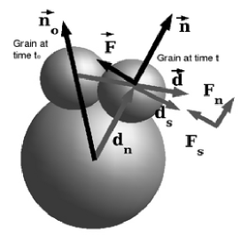
Figure 1: Interaction forces are decomposed in normal and tangential directions to the contact area.

$${\bf F}_{s}=-{\rm min}\left(|\kappa_{s}\zeta|,\mu|F_{n}|\right)sign(\zeta){\bf\hat{s}},$$ (2)

The shear force ${\bf F}_{s}$ in Eq. 1 depends on contact history and cannot be entirely determined by the position of grains. Such force is given by Eq. 2, where the tangential stiffness is $\kappa_{s}=8a_{c}G/(2-\nu)$, shear modulus of the grains is given by $G$ and $\nu$ is the Poisson’s coefficient. The term $a_{c}$ denotes the radius of contact area previously defined and $\mu$ represents the Coulomb friction coefficient. The term $\zeta$ denotes the component of the relative displacement vector in the tangential direction that took place since the time $t_{0}$, when the contact was established.

$$\zeta(t)=\int_{to}^{t}v_{s}(t^{\prime})dt^{\prime},$$ (3)

where $v_{s}={\bf v}_{ij}\cdot\hat{\bf s}$ and $\hat{\bf s}=\vec{\zeta}/|\vec{\zeta}|$. The vector ${\vec{\zeta}}$ can be computed from the displacement vector d between the grains ${\vec{\zeta}}={\bf d}-({\bf d\cdot n}_{0}){\bf n}_{0}$ (see Figure 1).

At this stage, periodic boundary conditions are imposed on gravity perpendicular directions to emulate an effectively larger system and the underground natural confinement of rocks in those directions.

The initial pack models a high porosity $\phi=41.2\%$ sand, where contacts involve marginal contact areas. The size of the generated sample was $8\times 8\times 32$ in units of maximum grain diameter. Following previous results (García et al., 2004), this volume is several times larger than the minimum homogenisation volume for the porosity of a sample with the given grain size distribution.

Samples with different packing are obtained by simulating the naturally occurring compaction of sediments. Following García et al.(2004), this process is simulated by displacing towards the sample core, grains contained in frozen slabs at both ends of the sample in the $\hat{z}$ direction. Once such macroscopic strain in imposed, ample time is allowed for grains to rearrange and relax accumulated stress.

III.2 Cementation model

Once the initial sand pack is obtained, the cementation process is simulated in several steps representing different stages in the sand diagenetic history. At each step, a volume of cement is added at specific locations within pores. Cement is added in three different manners that model cement with distinct origins and their micro-geometric implications.

The procedure followed to add cement starts by discrediting the three dimensional sample into cubic boxes of side length $c_{w}\approx R/10$, $R$ being the average radius of matrix grains. The set of cells intersects the sample voids and solid matrix, but just those cells whose centre coincides with pore space are potential locations for cement. Cells are subdivided into three groups:

1. Contact cells are those that intersect two or more grains. These, are located near grain contacts at the sharpest zones of pore space.

2. Surface cells are those centred in pore space and contacting with at least with single grain. Contact cells are a subset of surface cells.

3. Body cells are those centred in the pores without intersecting any grain.

In practise, cement is added by marking as cement saturated a fraction of pore centred cells. This mark is achieved by locating a cement particle at the centre of the cell. Each cement particle represents a cubic subvolume in the sample where cement is allocated.

III.3 Contact Cement

To model the microgeometry associated with contact cement model, we propose an algorithm of several steps that represent a different stage in the diagenetic history of the sample. Each step involves porosity reduction due to the addition of cement to pores. First, a small fraction of contact cells is marked as cement saturated. During the following steps, an increasing number of contact cells are filled with cement until no contact cells are left.

In practise, a cell are marked as cement saturated by adding a single cement particle to the centre of the cell. As this particle represents a cubic subvolume $c_{w}^{3}$ of cement within the sample, we assign to it a mass $m_{c}=\rho_{c}c_{w}^{3}$, where $\rho_{c}$ is the volumetric density of the cementing material.

After all contact cells are filled, further cementation steps involves the addition of cement to selected cells, neighboring those previously filled. First, we list all empty neighboring cells of those already filled with cement. Then, among these empty cells we select those lying closer to the grain matrix, and fill them with a new cement particle. Thus, when all contact cells are filled, this procedure promotes the cement accumulation from contacts to surface cells.

A sequence of steps where cement was added according to the described procedure is shown in Figure 2. the Figure shows a two dimensional example for illustrative purposes. However, results reported here refer to three dimensional samples and smaller cells (cells width $c_{w}\approx$ $1$ $th$ of average grain radius).

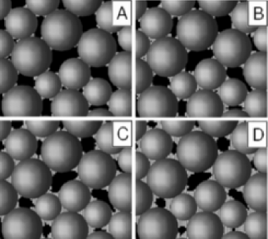
Figure 2: Figures $A$,$B$: an increasing number of contact cells is filled with cement until no contact cells left. Then, cement grows from contacts to surfaces in Figures $C$ to $D$. In the Figure, $2D$ samples are shown for clarity. Nevertheless, results reported here refer to the three-dimensional samples.

III.4 Coating cement

To model the microstructure related with coating cement, we mark each cell with an index proportional to its distance to the solid surface. At each cementation step, all empty cells are checked and those with the smallest index (closest to matrix surface) are filled with a cement particle. In the first steps, cementing material is added on grain surfaces. As is shown in Figure 3, further cementation steps add cement deeper into the pore bodies so that rims appear around grain surfaces.

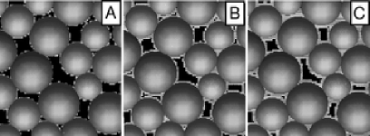
Figure 3: From step $a$ to $c$ cement is added to grain surfaces as a coating. This procedure simulates the homogeneous precipitation of solid material on the surface of pores. Figure shows a two dimensional case for clarity, reported results are for three dimensions though.

The successive cementation steps simulate several stages of the cementation history of the sample, where a change in the chemical equilibrium conditions causes precipitates to deposit uniformly on the grain surface.

III.5 Pore body cement

Simulation of pore body cements begins with the addition of cement particles to a fraction of surface cells selected at random. In the following steps, we check the empty cells contacting those already filled with cement. Each empty cell is then filled with a cement particle according to a probability $p$, proportional to the cell distance to grain surface. This procedure, simulates a preferential grow of cement from grains surface to pore bodies.

As shown in Figure 4, the initial cemented cells behave as seeds for clusters that grow from the grain surface to pore bodies. The described procedure guarantees the continuity of the cement phase and simulates cementing materials in the form of long crystals attached to grain surfaces.

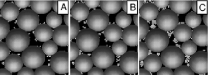
Figure 4: Figure $a$: initial seed of cement. Figures $b,c$: further cementation steps when cement is added preferentially at pore bodies. Figure shows a two dimensional cases for clarity. However, results refer to three dimensional samples.

Cell width defines the resolution limit of the simulations. If cells are too wide, poor resolution is obtained and porosity decreases sharply to zero after a few cementation steps. Small cells allow more control of the final porosity of the sample at expenses of an increase in the computational cost. More details about the effect of resolution on the computational cost are found in the appendix B.

III.6 Interaction

After a given porosity is reached due to cementation, we simulate the acoustical pulse transmission through the sample using Molecular Dynamics techniques. As Molecular Dynamics involves the explicit solution of Newton’s equations of motion for a particle based system, we need to consider the interaction forces between the particles of the different constituents of the aggregate. In our model, particles conform the quartz matrix and cement. We do not consider fluid particles that may be in pore volume. This approximation is justified if we suppose the fluid saturating pores to be air free to drain while sample strains. The effect of a more incompressible saturating fluid such as water or oil could be included and it is proposed for future work. In this way, our simulation techniques allow us to isolate the acoustical effect of cement from other agents that modify the acoustics of a real sample. With this approximation, we need only consider three kinds of interaction forces between particles: grain to grain forces, interaction between cement particles, and interaction forces between cement particles and grains.

In our model, the addition of cementing material is assumed not to disrupt the internal stress state of the sample. This assumption is justified since cementation is a relatively slow process when compared to compaction (Bernabé et al., 1992). Therefore, cement is added to pores at mechanically stable locations after grain-to-grain contacts are formed. When a perturbation of this equilibrium state occurs, changes in the internal stress field of the sample are produced. At the pore scale, grains change their relative positions and interparticle forces change by an amount $\Delta{\bf F}_{c}$ with respect to the initial equilibrium network.

If after a perturbation a pair of contacting grains labeled $1$ and $2$ at positions ${\bf r}_{1}$ and ${\bf r}_{2}$, displace to ${\bf r}_{1}+{\bf dr}_{1}$ and ${\bf r}_{2}+{\bf dr}_{2}$ respectively, their relative displacement is calculated as ${\bf d}={\bf dr}_{2}-{\bf dr}_{1}$. The component of the displacement along the normal direction of the contact is given by $\Delta\xi={\bf d}\cdot{\bf\hat{n}},$ being ${\bf\hat{n}}=({\bf r}_{2}-{\bf r}_{1})/|{\bf r}_{2}-{\bf r}_{1}|$ the unit vector joining grains centre at equilibrium. The tangential displacement is calculated as $\vec{\Delta\zeta}={\bf d}-({\bf d}\cdot{\bf\hat{n}}){\bf\hat{n}}$. This vector defines the tangential direction ${\bf\hat{s}}=\vec{\Delta\zeta}/\Delta\zeta$ with $\Delta\zeta=|\Delta\vec{\zeta}|$. During this stage, the force change ${\bf\Delta F}_{c}$ due to relative displacement of contacting grains is computed according to:

$${\bf\Delta F}_{c}=\{(k_{n}\Delta\xi-\gamma_{n}\dot{\Delta\xi})\}{\bf\hat{n}}+{\bf\Delta F}_{s}.$$ (4)

Term $\kappa_{n}$ in Eq. 4 is the elastic stiffness for normal deformations, defined previously in equation 1. However, in this stage we assume a negligible change in the contact area due to the acoustic pulse. This approximation constitutes a linearization of Hertz force, that represents the normal grain$-$grain elastic interaction that acts on contact. The second term in braces in Eq. 4, describes the viscous forces for normal deformations. In our simulations, we have adjusted this parameter to obtain a normal restitution coefficient $e_{n}=0.9$, in agreement with experimental results (Kuwabara and Kono, 1987; Schafer et al., 1996).

The term ${\bf\Delta F}_{s}$ in Eq. 4 represents the change in shear force. To compute this term, we assume that no sliding between grains occurs during pulse transmission. In such case, shear force is considered viscoelastic and calculated according to

$${\bf\Delta F}_{s}=\{k_{s}\Delta\zeta-\gamma_{s}{\dot{\Delta\zeta}}\}{\bf\hat{s}}.$$ (5)

The first term in the Eq. 5 represents the elastic component of the shear force. As no sliding is assumed, the tangential stiffness is computed according with Hertz-Mindlin theory $\kappa_{s}=4a_{c}G/(2-\nu)$. The term $G$ denotes the grains’ shear modulus, $\nu$ is the material Poisson’s ratio and $a_{c}$ is the radius of the initial contact area defined previously. The second term in the Eq. 5 represents the viscous forces for shear deformations. Parameter $\gamma_{s}$ was adjusted to obtain a tangential restitution coefficient $e_{s}=0.9$. The parameters to compute forces, were chosen to model quartz sand grains (see Table 1).

Table 1: Parameters used in Eq. 4 and 5 to compute forces between quartz grains (Mavko et al., 1988).

Parameter	Symbol	Value
Density$(gr/cm^{3})$	$\rho_{g}$	2.65
Shear modulus(GPa)	$G$	44
Poisson coefficient	$\nu$	0.08
Friction coefficient	$\mu$	0.3

To compute forces between cement particles, we follow a procedure described by O’Brien and Bean (2004). In this procedure, cement particles are considered as nodes on the cubic lattice that discretise the sample. When a cement particle displaces from its initial position on the lattice, it interacts with its $18$ closest neighbours in the lattice as shown in Figure 5. This interaction force is calculated according to:

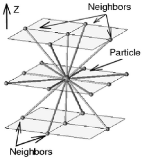
Figure 5: Each cement particle interacts with cement particles present in each of its closest eighteen nodes. Interaction force is decomposed in a component that acts along the line joining cells centre and a bending term.

$${\bf f_{c}}=C_{n}\left[{\bf u}_{12}.{\bf\hat{n}}\right]{\bf\hat{n}}+\frac{C}{|{\bf x}_{12}|^{2}}{\bf u}_{12},$$ (6)

where ${\bf x}_{12}$ denotes the vector joining particles $1$ and $2$ on the undisturbed lattice and ${\bf\hat{n}}={\bf x}_{12}/|{\bf x}_{12}|$. The vector ${\bf u}_{12}$ denotes the relative displacement of particles from their relative positions on the undisturbed lattice. The first term is the normal force with elastic constant $C_{n}$. The second term in Eq. 6 is the bending term and $C$ is an elastic constant for the interaction (O’Brien and Bean, 2004). The force given in Eq. 6 can be expressed in a form similar to Eq. 4. However, we decided to remain as close as possible to the original reference for clarity.

Following O’Brien and Bean (2004), energy of the elastic lattice can be compared with the elastic energy of an elastic continuous. The shear elastic modulus $G_{c}$ and Lamé constant $\lambda_{c}$ of the lattice can be expressed in terms of $C_{n}$ and $C$ according with the relation:

$$\begin{array}[]{l}\lambda_{c}=\frac{C_{n}}{c_{w}}-\frac{2C}{c_{w}^{3}},\\ \\ G_{c}=\frac{C_{n}}{c_{w}}+\frac{2C}{c_{w}^{3}},\end{array}$$ (7)

where $c_{w}$ is the lattice parameter (in our simulations $c_{w}\approx 1$ $th$ of average grain radius).

$$\begin{array}[]{l}V_{pc}^{2}=\frac{1}{\rho_{c}}\left(\frac{3C_{n}}{c_{w}}+\frac{2C}{c_{w}^{3}}\right),\\ \\ V_{sc}^{2}=\frac{1}{\rho_{c}}\left(\frac{C_{n}}{c_{w}}+\frac{2C}{c_{w}^{3}}\right).\\ \end{array}$$ (8)

From linear elasticity, it is possible to express the wave velocities in the cement phase as in Eq. 8, where $V_{pc}$ and $V_{sc}$ are respectively the $P-$wave and $S-$wave velocity of the cementing material. The term $\rho_{c}$ is the volumetric mass density of cementing material. As each cement particle represents a cubic subvolume $c_{w}^{3}$ of cement, such density is related to the mass of cement particles $m_{c}$.

$$\begin{array}[]{l}C_{n}=\frac{1}{2}\rho_{c}\left({V_{pc}}^{2}-{V_{sc}}^{2}\right)c_{w}\\ \\ C=\frac{1}{4}\rho_{c}\left(3{V_{pc}}^{2}-{V_{sc}}^{2}\right){c_{w}}^{3}\\ \\ m_{c}=\rho_{c}c_{w}^{3}.\\ \end{array}$$ (9)

For a cement of given mass density $\rho_{c}$ and wave velocities $V_{pc},V_{sc}$, the mass of cement particles $m_{c}$ and elastic constants in Eq. 6 are determined through Eq. 9. In our simulations, we considered the hard cement and soft cement limits compared to quartz. Parameters used in both cases are shown in Table 2. The hard cement case, models a quartz-like cement such as that formed by quartz dissolution of matrix grains. Soft cement models a material added to pores such as soft clays. To simplify, we considered the same volumetric mass density for cement in both cases.

Table 2: Elastic parameters and mass density used to model different cementing materials.

Parameter	Symbol	Hard cement	Soft cement
P-Velocity$(Km/s)$	$V_{pc}$	3.0	1.5
S-Velocity$(Km/s)$	$V_{sc}$	1 .8	0.9
Density$(gr/cm^{3})$	$\rho_{c}$	2.65	2.65
Poisson Coef.	$\nu_{c}$	0.22	0.22

The third kind of interaction force arises when grains displace relative to cement particles contacting their surface. This interaction in also computed by Eq.4, but the elastic constants $\kappa_{n}$ and $\kappa_{s}$ are now computed considering the Young’s modulus and Poisson coefficient of quartz and cement. The diameter of contact area is taken as the cement cell width $c_{w}$. In this manner, a grain feels a force due its contacting grains and due to cement particles contacting its surface.

III.7 Acoustics

In order to perform acoustic tests, the sample is subdivided along the propagation axis $\hat{z}$ into parallel slabs of $2$ largest grains diameters. A square wave displacement is imposed on grains contained in one end slab of the sample while the other ending slab is kept fixed as is shown in Figure 6. The former boundary condition, emulates the setup of an acoustic measurement. The fixed boundary condition on the opposite end prevents the sample from displacing as a whole.

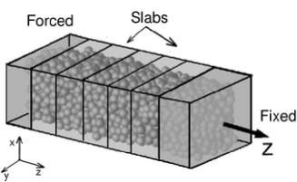
Figure 6: Sample volume is discretised into parallel slabs along $\hat{z}$ axis. At one end, a square wave displacement is imposed while the opposite slab is frozen. Average forces on grains contained in each slab are calculated as function of time to track pulse position and amplitude.

The imposed strain displaces grains from their original equilibrium positions and disrupts the initial force network. This perturbation propagates in the form of an acoustic pulse with a well defined central frequency. To keep track of the pulse position and amplitude, we monitor changes in the forces felt by grains as function of time and position. The average of the force along $z$ over the grains contained in each slab at time $t$ is taken as the acoustical signal $A(z,t)$ at the position of the slab centre $z$. This value is calculated according with the relation:

$$A(z,t)=\frac{1}{N_{i}}\sum_{i}^{N}{f_{i}},$$ (10)

where term ${f_{i}}$ is the force change at time $t$ on the $ith$ grain or cement particle in the slab. The summation index runs over the $N$ particles in the slab. This procedure simulates a set of acoustical detectors distributed along the sample.

As Figure 7 shows, the position in time of the stress pulse can be tracked by comparing signals received in different detectors.

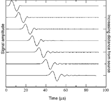
Figure 7: Signals recorded, at the simulated acoustical detectors, correspond to the average force along $\hat{z}$ of grains and cement particles in different slabs of the sample. From top to bottom, signals are recorded at detectors located increasingly farther from the source.

$$V_{p}=\frac{L}{T_{2}-T_{1}}+-\frac{L\Delta T+T\Delta L}{(T_{2}-T_{1})^{2}},$$ (11)

Mean pulse velocity $V_{p}$ is calculated according to Eq. 11, by comparing the arrival times $T_{1}$ and $T_{2}$ of the signal maximum in two detectors separated by a distance of $L$. The error in pulse position $\Delta L\approx R$ is estimated as the half width of slabs $\approx 2R$. Error in time arrival $\Delta T$, is taken as the time spacing between two consecutive calculations of force average in the slabs.

IV Results

We simulate the acoustic pulse propagation through a cemented sand. Cement is preferentially added near grain-to-grain contacts following the procedure described in section III.3 and its elastic properties are given in the column labeled as Hard Cement in Table 2. These parameters are suited to model a quartz-like cement and common used cements in experiments. This initial system mimics a well sorted and non compacted sand with porosity $\phi=41.2\%$ and point grain-to-grain contacts. We refer to this system as the non-compacted sample. Porosity reduction of the initial high porosity sample is achieved in several steps in which varying amounts of cement are added within pores. Acoustic pulse propagation is simulated for different degrees of cement saturation $S_{c}$.

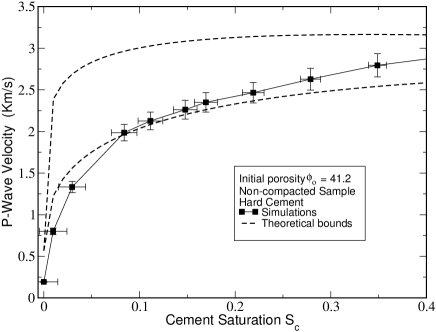
Figure 8: Small amounts of contact cement contributes to increase stiffness of the composite. As more cement is added, it locates farther from contacts and stiffness increases at an smaller ratio. Consequently, $V_{p}(S_{c})$ trend shows a characteristic downward concavity.

As shown in Figure 8, we observe an increase in sound velocity when an small amount of cement is added preferentially near grain contacts. This trend occurs because cement increases the restoring force of contacts and bridges grains initially separated. As a result, stiffness of the sample increases at a higher rate than porosity is reduced. Consequently, $V_{p}$ trend shows a downward concavity. As has been pointed before by Dvorkin and Nur (1996), this is a consistent explanation to some observed high porosity-velocity samples.

When more cement is added, porosity reduces and particles tend to locate progressively farther from contacts. In this case, stiffness increases at an slower rate than in the higher porosity range, when cement particles locate precisely at contacts. The net result is a decreasing slope of the velocity-porosity curve as porosity is reduced.

To compare our results with effective medium approximations (Dvorkin et al., 1994a; Dvorkin and Nur, 1996), we plot in Figure 8 the theoretical bounds for the sound velocity of the cemented sample. Both theoretical curves were obtained with the formulae given in appendix A for the simulation parameters. The upper trend (high velocity) corresponds to the idealised case when all cement is precisely added at contacts. The low velocity trend, corresponds to the scheme in which cement is added uniformly on the grain surface.

As shown in the Figure 8, obtained velocity-porosity trends for the non-compacted sample with contact cement, have the same qualitative behaviour than theoretical predictions. However, theory predicts a sharp velocity rise when small amount of cement is first added. Beyond the initial velocity rise, theoretical curves tends to saturate. Instead, we observe a soft continuous velocity increase with cement saturation $S_{c}$.

For a set of parameters close to ours, previous experimental studies reported a similar qualitative behaviour for a system of beads cemented with solidified epoxy (Hezhu, 1992; Dvorkin et al., 1994a), but the experimental results lay between both theoretical curves (Dvorkin et al., 1994a). We attribute this discrepancy with our results, to the stiffness of the initial uncemented sample. Theoretically, a finite non vanishing velocity is expected for the uncemented samples regardless of the effects confining pressure. For the case shown in the Figure 8, the minimal theoretical velocity is higher than that obtained in our simulations. Experimentally, results in the aforementioned experiments deal with compacted samples, that uncemented, propagate sound at velocities higher than the minimum predicted in the theory (Hezhu, 1992). On the other hand, in our settling algorithm grains settle due gravitational forces and no confining pressure is applied. As a result, we obtain very loose samples with marginal contact areas where P-Wave velocity can be quite smaller.

With the aim to better reproduce common experimental setups used for rocks, we simulated the compaction of the uncemented sample to a porosity $\phi=38.6\%$. At this porosity, confining pressure was recorded as $P_{c}\approx 30MPa$ and sound velocity was observed to increase from $V_{p}=0.2Km/s$ to $V_{p}=1.7Km/s$, similar to the minimal velocity reported in the aforementioned experiments (Dvorkin et al., 1994a). Then, the cementation process was simulated as in the previous case and acoustic tests were performed for different cement saturations.

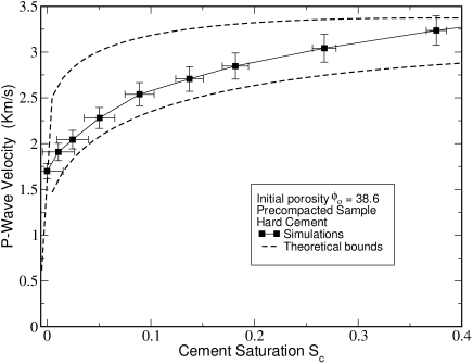
Figure 9: Pulse velocity for different cement saturations. Uncemented sample is compacted with $30MPa$ confining pressure. After compaction, cement is added preferentially near contacts. Theoretical predictions can be good estimates of velocity bounds for precompacted samples.

As expected, Figure 9 shows that for zero cement saturation, velocity is higher in the compacted sample than in the uncompacted sample. Additionally, the Figure shows that in the case of the compacted sample, velocity increases at a slower rate when cement saturation $S_{c}$ increases. The net result is that the velocity trend for the compacted sample lies between theoretical curves. In this case, for the range of cement saturation $S_{c}$ shown in the Figure 9, obtained results are in good quantitative agreement with available experimental data reported in previous works (Hezhu, 1994; Dvorkin et al., 1994; Dvorkin and Nur 1996). It should be noted that for the case of the compacted sample, theoretical curves are slightly different from those of the uncompacted sample, since coordination and porosity are different. Nevertheless, these variations are relatively small.

These results suggest that confining pressure of the initial uncemented sample is a crucial parameter which determines the velocity trends obtained after adding small amounts of cement. This is an intuitive result since for loose sediments close to suspension, stiffness can be negligible. Then, any stiffness increase due to cementation can be several times the initial one and represent a large fraction of the final stiffness of the cemented sample. When samples are previously compacted, the initial hosting medium for the cement becomes stiffer (despite fracturing). In this case, further addition of small amounts of cement can represent an smaller fraction of the final stiffness of the sample.

Results in Figure 8 and Figure 9, suggest that contact cement theory may work well for samples which are cemented after some compaction is achieved. However, it may overestimate sound velocity for the case of cement added to weakly compacted media. The latter case, can be that of artificially cemented granular materials such as young sediments cemented with perforation mud, or laboratory produced materials. We believe that the case where cement is added after some compaction is the most realistic for rocks, since chemical cementation is achieved after some pressure-temperature conditions are reached with burial.

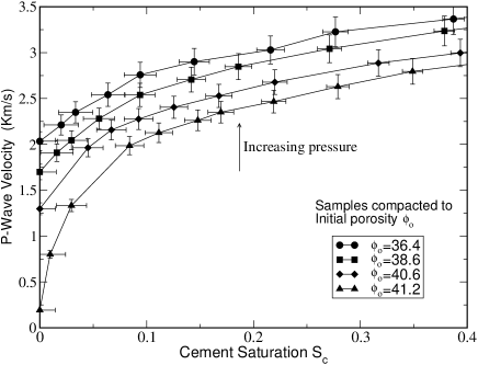
Figure 10: Each curve represents a possible diagenetic path for a granular material. Samples are first compacted to a porosity $\phi_{o}$ due to burial. Then, cementation process begin. The more compacted the samples, the smaller the relative increase of velocity with $S_{c}$.

This behaviour is further illustrated in Figure 10 where results are shown for several cases in which cementation starts after some compaction. In this Figure, each trend may represent a possible diagenetic path followed by a granular material. The starting framework in all cases is that of a very loose material of porosity $\phi=41.2\%$, representing sediments after settling. The initial loose pack is then compacted to a porosity $\phi_{o}$, simulating the mechanical effects of burial. After compaction, a relatively hard cementing material is added in varying amounts.

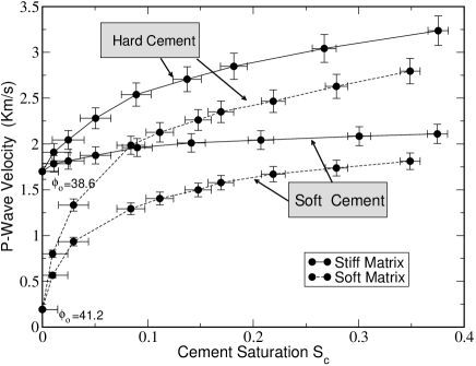
Figure 11: Velocity increase in soft samples depends mainly in the amount of cement. For stiff samples, velocity increase depends strongly on the elastic properties of cement.

As shown in Figure 11, we observed the same qualitative behaviour when considering cementing materials with different elastic properties. In the Figure, sound velocity in the uncompacted sample increases by a factor of $\approx 10$ when a relatively hard cement saturation varies from $0-0.1$. For the same cement saturation, a relatively soft cement increases sound velocity in a factor of $\approx 7$. In the case of a compacted (stiffer) sample, this variation approximates to $\approx 25\%$ in the case of the hard cement and $\approx 12\%$ for the soft cement. According with these results, velocity rise in soft samples mainly depends on the amount of cement while in stiff samples the most relevant factor is the type of cement.

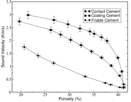
Figure 12: Acoustical response depends on microstructure details. Contact cement leads to a downward concavity in $V_{p}(S_{c})$ trend with decreasing slope as cement saturation increases. Friable cement leads to the opposite behaviour. Coating cement corresponds to an intermediate case.

Cements can also accumulate as a coating cement on grain surfaces, or at pore bodies far from contacts. The former, can be the case when cement precipitates as a solid material in low flux zones (Manmath and Lake, 1995). The latter case, is encountered in some sands which held together by confining pressure only. Following (Dvorkin and Nur, 1996), this kind of cement is termed here as friable or pore body cement. This geometric character of cementation process can be explored in our simulations by following details given in section III.4 for coating cement and section III.5 for friable cement. Methods to simulate the case of cement at contacts, treated previously, are discused in section III.3.

In Figure 12, the lowest velocity trend is obtained when solid cement is added preferentially as pore-filling material. Since this kind of cement accumulates far from contacts, it contributes marginally to rock stiffness. The main effect of this kind of cement is to reduce porosity. As more pore-filling material is added, cement particles start to bridge separated grains. Then, blocks of cement particles are also compressed during pulse propagation with the net effect of an increasing slope of velocity trend as porosity reduces.

It is to be noticed that if clays were added during settling, we should expect a different behaviour. In that case, above a critical concentration of clays (about $\approx 40\%$), they become load-bearing and completely surround disconnected quartz grains. In such case, soft clays dominate the acoustics and velocity decrease for porosities below some thereshold value (Hezhu, 1992).

In the case treated here, Figure 12 shows a monotonic velocity increase with cement saturation. Here, clays or any other cementing material is added after settling. Therefore, quartz grains remain in contact in the whole porosity range. As a consequence, soft clays may reduce porosity but sound velocity can only decrease slightly due to inertial effects. This result suggests that for low porosity sands with high clay content, high sound velocity should be expected if clays are of diagenetical origin. Low porosity-velocity can be related to the depositional origin of clays. This may be an important factor to consider when reconstructing the history of a reservoir sample.

The velocity trend for coating cement lies in between limiting cases of friable and contact cement. In this case, a fraction of cement deposits near contacts and contributes to rock stiffness, while a significant volume of cement mainly reduces porosity. Figure 12 shows that for the same porosity, this kind of cementation leads to higher velocities than those of friable sand and lower velocities than those of the contact-cemented sample. These results show that microstructural details are very important parameters which influence in the velocity-porosity trends of cemented samples.

To further compare our results with available experimental data, we calculated the P-Wave modulus from results in Figure 12. Computed moduli are shown against porosity in Figure 13.

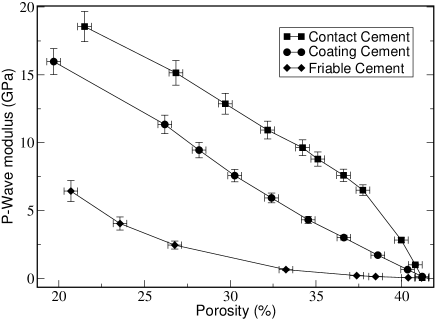
Figure 13: In the medium to high cement saturation, contact cement leads to a quasilinear trend for P-Wave modulus with porosity in agreement with experimental results (Dvorkin et al., 1994b). Coating cement and friable sands shows an upward concavity observed in some naturally occurring sands (Dvorkin and Nur, 1996).

As expected, results in Figure 13 show different trends for P-Wave modulus depending on the amount of cement and cementation scheme. In the case of contact cement, a quasilinear trend is observed for cement saturations above $\approx 10\%$. This result, qualitatively coincides with previous experimental results reported in (Dvorkin et al., 1994b) and references therein. Similar behavior was observed for the case of coating cement. Nevertheless, P-modulus is smaller for the range of cement saturation studied. Velocity trends obtained for the case of friable cement can be compared with experimental data obtained for some samples with scarce intergranular cement (Dvorkin and Nur, 1996). These results are in good agreement with the varios correlations between P-modulus and porosity observed in reservoir sands.

It must be noted that details of microstructure are hardly included in most theoretical approximations. Some models treat the case of two a phase composite and/or spherical inclusions, being useless in the range $0\%<S_{c}<100\%$. For instance, Hashin-Shtrikman model establish bounds to the maximum and minimum elastic moduli at zero porosity ($S_{c}=100\%$). Although a generalization of this model would allow us to calculate bounds for the moduli at intermediate porosities (Mavko et al., 1988), in our simulations and in the experiments considered, voids are filled with air with negligible elastic modulus. In this case, lower bound for the moduli is trivial(zero) in all the range of cement saturation considered. Although Contact Cement Model explicitly includes the microstructure, some the assumptions made in the theory are not supposed to be valid for large amounts of cement.

V Conclusions

Simulation results show that cements modify elastic properties of sands in different manner, depending on the relative stiffness of cement and the hosting medium, the amount of cement and its localisation within pores.

If cement is added preferentially near contacts, it can contribute noticeably to the stiffness of the composite, the effect being enhanced in uncompacted granular samples. Friable cement leads to relatively low velocity samples even when for moderate cement saturations. Velocity trends show characteristic concavities in each case.

As confining pressure increases, the hosting medium for the cement becomes stiffer by compaction and cements have an smaller effect on the sound velocity of the final composite. As a result, velocity-porosity trends differ for samples that follow different compaction-cementation paths. Although contact cement theory does not account for the confining pressure effects, it can give a good estimate for the sound velocity in precompacted samples with small amounts of contact cement($S_{c}<15\%$).

Simulation results presented, qualitatively and quantitatively reproduce the available experimental data where porosity reduces and velocity increases due to cementation. The proposed methods, are suited to take into account the microstructural details of cementation process and their acoustical implications. As these details are hardly included in most effective medium approximations, simulation techniques can be considered an alternative tool to model the acoustics of cemented sands and to get new insights on the underlying physics behind the phenomena.

Nomenclature

$FZI$ Geometric index to characterise microstructure

$P_{s}$ Pore shape related value

$S_{v}$, Pore specific surface

$\tau$ Tortuosity

${\bf F}_{c}$ Contact force

${\bf F}_{n}$ Hertz Force for a pair of grains in contact

${\bf F}_{s}$ Shear force of a grain-to-grain contact

${\bf\Delta F}_{s}$ Change in Shear force due to a perturbation

${\bf\Delta F}_{n}$ Change in Normal force due to a perturbation

$\Delta{\bf F}_{c}=\Delta{\bf F}_{n}+\Delta{\bf F}_{n}$

$a_{c}$ Radius of the contact area

$E_{i},E_{f}$ Young modulus of grain $i$ and effective Young modulus for a contact

$\kappa_{n}$ Hertz normal stiffness of a contact

$\kappa_{s}$ Shear stiffness of a grain-to-grain contact

${\bf\hat{n}}_{12}$ Unitary vector joining the centre of grains $1,2$.

$\hat{s}$ Unitary vector tangential to the contact

$\nu,\nu_{i},\nu_{c}$ Poisson coefficient of grains, particle $i$ and cement

$R,R_{f}$ Grain radius and effective radius for Hertzian contacts

${\bf r}_{i}$ Position vector of grain $i$

$\mu$ Poisson coefficient of dry friction between grains

$e_{n}$ Restitution coefficient for normal interaction

$\gamma_{n},\gamma_{s}$ Damping constants for normal and tangential directions to the contact.

$c_{w}$ Width of cells that discretise the sample

$\rho_{c},\rho_{g}$ Volumetric mass density of cement and grains

$\xi$ Overlapping between spheres in contact

$\xi_{0}$ Overlapping between spheres in mechanical equilibrium

$\zeta$ Relative displacement of contacting particles in direction tangential to the contact

$\zeta_{0}$ Relative displacement of contacting particles in direction tangential to the contact when particles are in mechanical equilibrium

$G$, $G_{c}$ Shear modulus of material composing grains and cement

$\lambda_{c}$ Lamé constant of cementing material

$C_{n}$ Normal stiffness for cement particles interaction

$C$ Elastic constant for the interaction between cement particles

${\bf x}_{12}$ Vector joining particles in the undisturbed cement lattice

${\bf u}_{12}$ Relative displacement of particles from their positions on the undisturbed lattice.

$m_{c}$ Mass of a cement particle

$V_{pc},V_{sc}$ P-wave and S-Wave velocities of cementing material

$V_{p}$ P-wave velocity of the grains and cement composite

$P_{c}$ Confining pressure

$\phi$ Porosity of the cemented sample.

$\phi_{o}$ Porosity before cementation.

$S_{c}$. Cement saturation

$K_{f},G_{f},M_{c}$ Bulk, Shear and Compressional modulus of cement

$\Omega$ Computational cost

$t_{c}$ Characteristic time for the interaction among particles

VI Acknowledgments

This work was supported by the IVIC Rocks project and by FONACIT through grant S1-2001000910.

Appendix A Effective medium approximation for cemented sands

According to the theoretical model proposed by Dvorkin et al. (1994a); Dvorkin et al. (1994b) and Dvorkin and Nur(1996), the initial porosity $\phi_{o}$ of an uncemented sample is decreased to $\phi$ by the addition of cementing material. Once a given volume of cement is added, the effective bulk $K_{f}$ and shear $G_{f}$ moduli of the composite is calculated according with Eq. 19.

$$\begin{array}[]{l}K_{f}=\frac{1}{6}N(1-\phi_{o})M_{c}\hat{S_{n}}\\ \\ G_{f}=\frac{3}{5}K_{f}+\frac{3}{20}N(1-\phi_{o})G_{c}\hat{S_{t}}\\ \\ M_{c}={V_{pc}}^{2}\rho_{c}\\ \\ G_{c}={V_{sc}}^{2}\rho_{c},\end{array}$$ (19)

where $\rho_{c},V_{pc},V_{sc}$ are mass density, P-wave and S-wave velocities of cementing material and $N$ is the average number of contacts per grain. The normal and tangential stiffness of the contacts in the cemented sample, denoted as $\hat{S}_{n}$ and $\hat{S}_{t}$ respectively, are given as function of porosity change due to cementation in Eq. 20 below.

$$\begin{array}[]{l}\hat{S}_{n}=A_{n}\alpha^{2}+B_{n}\alpha+C_{n}\\ \hat{S}_{t}=A_{s}\alpha^{2}+B_{s}\alpha+C_{s}\end{array}$$ (20)

where:

$$\begin{array}[]{l}\alpha=\left\{\begin{array}[]{ll}\left(\frac{2}{3}\frac{\phi_{0}-\phi}{1-\phi_{0}}\right)^{1/2}&\textrm{ for cement in layers}\\ 2\left(\frac{1}{3N}\frac{\phi_{0}-\phi}{1-\phi_{0}}\right)^{1/4}&\textrm{ for cement at contacts}\\ \end{array}\right\}\end{array}$$ (21)

The coefficients of the $\alpha$ powers in Eq. 20 are given in formulae 22:

$$\begin{array}[]{l}A_{n}=-0.024153{\Lambda}_{n}^{-1.3646}\\ B_{n}=0.20405\Lambda_{n}^{-0.89008}\\ C_{n}=0.00024649\Lambda_{n}^{-1.9864}\\ \\ A_{s}=-10^{-2}(2.26\nu^{2}+2.07\nu+2.3)\Lambda_{s}^{\omega_{1}}\\ B_{s}=(0.0573\nu^{2}+0.0937\nu+0.202)\Lambda_{s}^{\omega_{2}}\\ C_{s}=-10^{-4}(9.654\nu^{2}+4.945\nu+3.1)\Lambda_{s}^{\omega_{3}}\\ \\ \textrm{where}\\ \\ \omega_{1}={(0.08167\nu^{2}+0.4011\nu-1.8186)}\\ \omega_{2}={(0.027\nu^{2}+0.0529\nu-0.8765)}\\ \omega_{3}={(0.079\nu^{2}+0.1754\nu-1.342)}\\ \Lambda_{n}=\frac{2G_{c}}{\pi G}\frac{(1-\nu)(1-\nu_{c})}{1-2\nu_{c}}\\ \Lambda_{s}=\frac{G_{c}}{\pi G},\end{array}$$ (22)

where $\nu,\nu_{c}$ are respectively the grains and cement Poisson ratio, $G$ is the shear modulus of grains and the rest of symbols have the same denotation than in previous equation.

The theoretical predictions for the P-Wave velocity are then obtained for the cemented sample by substituting elastic moduli given in Eq. 19 in linear elasticity Eq. 23

$$V_{p}=\left(\frac{K_{f}+4/3G_{f}}{\rho_{f}}\right)^{1/2},$$ (23)

where $V_{p}$ is the sound velocity of the composite system of grains and cement and $\rho_{f}$ the effective mass density. In our simulations, we have used Eq. 23 to fit the obtained data.

Appendix B The effect of resolution in the computational cost

Resolution $\Omega$ affects computational cost in three different ways. First, cells width $c_{w}\approx R/\Omega$, being $R$ the average grain radii. As $\Omega$ increases, $c_{w}$ reduces and the number of cells to discretise the sample increases as $\approx\Omega^{3}$ in three dimensions. The larger the number of cells the larger the memory needed to store the information related with each cell. Additionally, as the number of cement particles raise, the number of operations to compute forces, velocities and actualise positions increases proportionally.

On the other hand, for smaller cells widths $c_{w}$, the mass of cement particles goes as $m_{c}\approx\Omega^{-3}$ and elastic stiffness constants goes as $\kappa\approx\Omega^{-1}$. The characteristic integration step $t_{c}$ is determined by the characteristic time related to interactions $t_{c}\approx(m_{c}/\kappa)^{1/2}\approx\Omega$. Therefore, as resolution $\Omega$ increases, the number of integration steps to simulate pulse propagation in the system during a unitary time rises linearly. As both the number of cement particles and integration steps increase, the computational cost is higher.

References

- (1) Adamson, A.W., Gast, A.P., 1982. Physical chemistry of surfaces. Willey Interscience, New York.
- (2) Bakke, S., Oren P.E., 1997. 3-D Pore-scale modelling of heterogeneous sandstone reservoir rocks and quantitative analysis of architecture, geometry and spatial continuity of the pore network. Society of petroleum engineering 35479, 35-45.
- (3) Bernabé, Y., Fryer, D.T., Hayes, J.A., 1992. The effect of cementation on the strength of granular rocks. Geophysical Research Letters 19 (14), 1511-1514.
- (4) Biswal, B., Manwart, C., Hilfer, R., Bakke, S., Oren P.E., 1999.Quantitative analysis of experimental and synthetic microstructures for sedimentary rock. Physica A 273 (3-4),452-475.
- (5) Bryant S., Cade, C., Mellor, D., 1993. Permeability prediction from geologic models. The American association of petroleum geologist bulletin 77 (8), 1338-1350.
- (6) Dvorkin J., Nur, A., Yin, H. 1994a. Effective properties of cemented granular materials. Mechanics of materials 18, 351-366.
- (7) Dvorkin, J., Nur, A., Yin, H. 1994b. Effective moduli of cemented sphere packs. Mechanics of materials 31, 461-469.
- (8) Dvorkin, J., Nur, A., 1996. Elasticity of high-porosity sandstones, theory for two North Sea datasheets. Geophysics 61, 1363-1370.
- (9) García, X., Araujo, M., Medina, E., 2004. Pwave velocityporosity relations and homogeneity lengths in a realistic deposition model of sedimentary rock. Waves in random media 14, 129-142.
- (10) Gundersen, E., Renand, F., Dysthe, D.K., Bjotlykke, K., Jamtveit, B., 2002. Coupling between pressure solution creep and diffusive mass transport in porous rocks. Journal of Geophysical Research 107, B11, 1-19.
- (11) Guodong, J., Patzek, T.W., Silin, D.B., 2003. Physics-based reconstruction of sedimentary rocks. Society of Petroleum Engineering 83587, 1-14.
- (12) Hezhu, Y., Dvorkin, J.,1994. Strength of cemented grains. Geophysical Research letters 21 (10), 903-906.
- (13) Hezhu, Y., 1992. Acoustic velocity and attenuation on rocks , isotropy, intrinsic anisotropy ans stress induced anisotropy. Ph.D. Thesis, Stanford University, Stanford, United States.
- (14) Kuwabara, G., Kono, K., 1987. Restitution coefficient in a collision between two spheres. Japanese Journal of Applied Physics 26, 1230-1233.
- (15) Love, A., 1944. A Treatise on the mathematical theory of elasticity. Dover Publications, New York.
- (16) Manmath, N., Lake, W.L., 1995. A Physical model of cementation and its effects on single-phase permeability. AAGP Bulletin 79 (3), 431-443.
- (17) Mavko G, M., Mukerji, T., Dvorkin, J., 1988. The Rock Physics Handbook. Cambridge University Press, Cambridge.
- (18) Nakagawa, K., Myer, L.R., 2001. Mechanical and acoustic properties of weakly cemented granular rocks. Energy citations database.
- (19) O’Brien, G.S., Bean J., 2004. A 3D discrete numerical elastic lattice method for seismic wave propagation in heterogeneous media with topography. Geophysical Research Letters 31 (14),L14608, doi:10.1029/2004GL020069, 1-4.
- (20) Prasad, M., 2003. Velocity-permeability relations within hydraulic units. Geophysics 68 (1), 108-117.
- (21) Rapaport, D.C., 1995. The art of molecular dynamics simulation. Cambridge University Press, Cambridge.
- (22) Schafer J., Dippel, S., Wolf, D.E., 1996. Force Schemes in Simulations of Granular Materials. Journal of Physics I 6, 5-20.
- (23) Schwartz, L.M., Kimminau, S.,1987. Analysis of electrical conduction in the grain consolidation model. Geophysics 52 (10), 1402-1411.