Normal state of a polarized Fermi gas at unitarity
Abstract
We study the Fermi gas at unitarity and at by assuming that, at high polarizations, it is a normal Fermi liquid composed of weakly interacting quasiparticles associated with the minority spin atoms. With a quantum Monte Carlo approach we calculate their effective mass and binding energy, as well as the full equation of state of the normal phase as a function of the concentration of minority atoms. We predict a first order phase transition from normal to superfluid at corresponding, in the presence of harmonic trapping, to a critical polarization . We calculate the radii and the density profiles in the trap and predict that the frequency of the spin dipole mode will be increased by a factor of 1.23 due to interactions.
Recent experiments on degenerate gases of 6Li with a mixture of two hyperfine species have explored the physics of Fermi gases experiment1 ; huletexp ; experiment2 and have led to a number of theoretical analyses theory1 ; yip ; mueller ; theory2 . One of the major experimental observations has been the occurrence of phase separation if the mixture contains more atoms of one species than of the other, i.e., if the gas is polarized. Some of the experiments suggest that in the unitary limit of strong interactions there are three phases: an unpolarized superfluid phase, a mixed phase which exhibits a partial polarization and a fully polarized gas. We now have a good understanding of the superfluid phase which has been the subject of numerous theoretical and experimental studies while the fully polarized phase is an ideal Fermi gas since atoms in the same spin state do not interact with each other. However, for intermediate polarizations, when both species are present, the nature of the mixed phase is not understood.
Here we study the mixed phase in the unitary limit by adopting an approach inspired by the theory of dilute solutions of 3He in 4He bardeen . We will assume that the majority species () forms a background experienced by the minority species () and that the latter behaves as a gas of weakly interacting fermionic quasiparticles even though the atomic interaction is very strong, being characterized by an infinite scattering length. In other words, we will assume that the system is a normal Fermi liquid, which will allow us to characterize the energy of the gas in terms of a few parameters and, by calculating these with a quantum Monte Carlo approach, allow us to make various predictions of experimental relevance.
We begin by writing the expression for the energy of a homogeneous system in the limit of very dilute mixtures and at zero temperature. The concentration of atoms is given by the ratio of the densities and we will take it to be small. If only atoms are present then the energy is that of an ideal Fermi gas , where is the total number of atoms and is the ideal gas Fermi energy. When we add a atom with a momentum (), we shall assume that the change in is given by
| (1) |
In other words, the atom in the gas behaves as a quasiparticle with a quadratic dispersion and an effective mass . In addition, there is a “binding” energy of the atom to the Fermi gas of atoms. This binding energy must be proportional to since there is no other energy scale in the unitary limit and we have used the factor for later convenience. We shall further assume that this quasiparticle is a fermion statistics .
When we add more atoms, creating a small finite density , they will form a degenerate gas of quasiparticles at zero temperature occupying all the states with momentum up to the Fermi momentum . The energy of the system can then be written in a useful form in terms of the concentration as:
| (2) |
Eq.(2) is valid for small values of the concentration , i.e. when interactions between quasiparticles as well as further renormalization effects of the parameters can be neglected.
In the following we will calculate and using a fixed-node diffusion Monte Carlo (FN-DMC) approach, already employed in earlier studies QMC1 ; QMC2 . We use the same attractive square-well potential to model the interactions between and atoms: for and otherwise. The short range is chosen as . The depth is fixed by the unitarity condition for the -wave scattering length and corresponds to the threshold for the first two-body bound state in the well: . For a single atom in a homogeneous Fermi sea of atoms the trial wave function , which determines the nodal surface used as an ansatz in the FN-DMC calculation, is chosen to be of the form boronat
| (3) |
where denotes the position of the atom and . In this equation the plane wave corresponds to the impurity travelling through the medium with momentum , where is the lenght of the cubic box and the are integers describing the momentum in each coordinate. Furthermore, is the Slater determinant of plane waves describing the Fermi sea of the atoms and the Jastrow term accounts for correlations between the impurity and the Fermi sea. The correlation function is chosen as in Ref. QMC1 . We consider a system of atoms and periodic boundary conditions. From the energy of the system with atoms we subtract the exact energy of the Fermi sea. The result is shown in Fig. 1 as a function of . From a linear best fit we obtain the following values: and which is consistent with the general inequality . We have checked that finite-size corrections associated with the number of atoms in the Fermi sea are below the reported statistical error. It is worth noticing that the binding energy of a single atom almost coincides with the average energy of an atom in the Fermi sea. A similar coincidence was found for the superfluid gap at unitarity Carlson .

A relevant question is to understand whether the equation of state (2) is adequate to describe regimes of large values of where interaction between quasiparticles and other effects might become important. To answer this question we have carried out a FN-DMC calculation of the equation of state at finite concentrations using the trial wave function
| (4) |
where and label, respectively, and atoms. The nodal surface of the wave function is determined by the product of Slater determinants and coincides with the nodal surface of a two-component ideal Fermi gas. As a consequence, the wave function in Eq. (4) is incompatible with off-diagonal long-range order (ODLRO) and describes a normal Fermi gas. In contrast, the BCS-type wave function used in Refs. QMC1 ; QMC2 is compatible with ODLRO and describes a superfluid state. A direct comparison between the groundstate energy of the normal and superfluid states can be carried out for equal numbers of and atoms, , with the result and showing the instability of the normal state for (see Fig. 2).
The results for the equation of state of the normal Fermi gas are shown in Fig. 2. To reduce finite-size effects we have considered closed-shell configurations =7,19,27,33 with =27,33. In Fig. 2 we also show the prediction of Eq.(2) based on noninteracting quasiparticles (dashed line). For small values of we find very good agreement, but for larger concentrations effects of interactions between quasiparticles start to be important and deviations from Eq.(2) become visible. The solid line is obtained from a polynomial best fit to the FN-DMC results.
From the equation of state of the mixed phase we can determine the transition between the fully polarized and the mixed phases as well as the transition between the mixed and the unpolarized superfluid phases psf . The equilibrium condition is obtained by imposing that the chemical potential and the pressure be the same in the two phases. It is useful to express the results in terms of the chemical potential and of the effective magnetic field . Here is the chemical potential of each spin species. The transition between the fully polarized and the mixed phase is second order and takes place at where we find , corresponding to . The transition between the mixed and the unpolarized superfluid phases is instead first order and is simply obtained via the standard Maxwell construction considering the tangent to the equation of state of Fig. 2 crossing the superfluid point at =1. We obtain the critical value at the transition. For smaller values of the system remains in the normal state, while above the critical concentration the system will begin nucleating the superfluid and phase separate into those two states. The phase transition is characterized by the value corresponding to Chevy . Note that at the critical value the difference between the best fit and the prediction of Eq.(2) is quite small so that this latter energy functional describes well the whole normal phase. This supports the idea that the normal state is a gas of weakly interacting quasiparticles. Eq.(2) would actually predict the value for the critical concentration, which corresponds to .

It is useful to compare the above results with BCS theory which also predicts 3 phases at unitarity yip ; mueller : a superfluid with energy , a mixed state which is a noninteracting partially polarized gas and a fully polarized gas. The mixed state energy is simply the kinetic energy and is an increasing function of . The tangent to the curve is at , corresponding to , thereby leading to a much reduced normal region with respect to the predictions of our FN-DMC calculation.
Now we turn to the trapped case. While we will discuss the situation only at zero temperature we should note that temperature can have an important effect on the density profile of the atoms. In experiments we usually have the condition . But since , we might be in a situation where and would therefore need to use the appropriate thermal distribution. With this caveat we turn to the inhomogeneous situation where we shall use the local density approximation (LDA) hulet . In a harmonic trap with potential , the local chemical potentials become . For small concentrations (in particular ), where only the normal state is present and where we can neglect the change in due to the attraction of the atoms, is the Thomas-Fermi density of an ideal gas whereas is a Thomas-Fermi profile with a modified harmonic potential . The potential seen by the atoms is more confining due to the attraction to the atoms. This also has consequences for the collective modes of the system: it leads us to predict that the spin dipole mode - the mode where the atoms oscillate as a whole in the midst of the atom cloud - will have a frequency given by
| (5) |
So, a direct measurement of the oscillation frequency of the atoms in a dilute mixture with would provide a useful test of this Fermi liquid theory and in particular of the numerical estimate of the parameters and damping .
For larger concentrations the system will exhibit a central superfluid core with chemical potential , whose radius in a spherical trap is given by
| (6) |
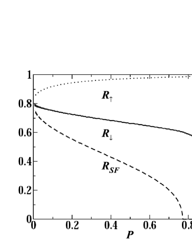
where is the radius of the component and is calculated at the transition point. In Fig. 3, we plot the radius of the superfluid component together with the radii of the minority and majority components, and respectively, in units of as a function of the polarization of the sample. We predict that the superfluid phase disappears at in good agreement with the experimental findings of experiment2 . Notice that as , while approaches the noninteracting value. In the opposite limit the radii converge to the known value . It is worth noticing that the BCS approach would predict the value at unitarity yip ; mueller pointing out the dramatic role played by the binding energy in the mixed state.
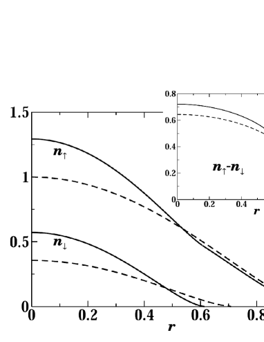
At the transition between the superfluid and the mixed normal phase the density of the two spin species exhibits a discontinuity, revealing the first order nature of the transition. The densities and jump from the superfluid value to the values and respectively, as one enters the normal phase. The discontinuity is an artifact of LDA and the inclusion of surface energy effects could In Fig. 4 we plot and as well as the difference as a function of position in a spherical trap when . These results, based on LDA, apply also to anisotropic traps through a simple scaling transformation. We find that both the total density and the density difference increase monotonically towards the center discrepancy . If then in the central superfluid region.
In conclusion, we study the polarized Fermi gas at unitarity as a normal Fermi liquid composed of weakly interacting quasiparticles associated with the minority atoms. These have a quadratic dispersion and, in the limit, have an effective mass with a binding energy , calculated with a FN-DMC approach. We derive an energy functional Eq.(2) with those parameters, assuming noninteracting quasiparticles and, using FN-DMC calculations at higher values of , show that corrections to the energy functional are small, even for relatively high concentrations. Assuming that no polarized superfluid phases exist, we predict a normal/superfluid first order phase transition at a critical value , corresponding, in the presence of harmonic trapping, to a critical total polarization . We also predict for small concentrations an increase by a factor of 1.23 of the frequency of the spin dipole mode with respect to the noninteracting value. A further application of the equation of state of the mixed phase could be, for example, the calculation of the dipole polarizability of the trapped Fermi gas dipole .
We acknowledge useful discussions with I. Carusotto, A. J. Leggett, L.P. Pitaevskii and N. Prokof’ev. We also acknowledge support by the Ministero dell’Istruzione, dell’Università e della Ricerca (MIUR).
References
- (1) G. B. Partridge, W. Li, R. I. Kamar, Y. Liao, and R. G. Hulet, Science, 311, 503 (2006); M. W. Zwierlein, C. H. Schunck, A. Schirotzek, W. Ketterle, Nature 442, 52 (2006); M. W. Zwierlein, W. Ketterle, cond-mat/0603489.
- (2) G. B. Partridge, W. Li, R. I. Kamar, Y. Liao, R. G. Hulet, cond-mat/0605581.
- (3) Y. Shin, M. W. Zwierlein, C. H. Schunck, A. Schirotzek, and W. Ketterle, Phys. Rev. Lett. 97, 030401 (2006).
- (4) J. Carlson and S. Reddy, Phys. Rev. Lett. 95, 060401 (2005); P. Pieri and G. C. Strinati Phys. Rev. Lett. 96, 150404 (2006); D. E. Sheehy and L. Radzihovsky, idem 060401 (2006); J. Kinnunen, L. M. Jensen, and P. T¨orm¨a, idem 110403 (2006), and cond-mat/0604424; M. Haque, H.T.C. Stoof, cond-mat/0601321; W. Yi and L.-M. Duan Phys. Rev. A 73, 031604(R) (2006) and cond-mat/0604558; K. Machida, T. Mizushime and M. Ichioka, cond-mat/0604339; M. M. Parish, F. M. Marchetti, A. Lamacraft, B. D. Simons, cond-mat/0605744; T. N. De Silva, E. J. Mueller, cond-mat/0604638 and cond-mat/0607491; F. Chevy, Phys. Rev. Lett. 96, 130401 (2006); A. Bulgac, M. M. Forbes, cond-mat/0606043; M. Iskin, C. A. R. Sa de Melo, cond-mat/0604184; C. Chien, Q. Chen, Y. He, K. Levin, cond-mat/0605039; K. B. Gubbels, M. W. J. Romans, H. T. C. Stoof, cond-mat/0606330.
- (5) C.-H. Pao, S.-K. Yip, J. Phys. C: Condens. Matter 18 5567 (2006).
- (6) T. N. De Silva, E. J. Mueller, Phys. Rev. A 73, 051602(R) (2006).
- (7) F. Chevy, cond-mat/0605751.
- (8) see e.g. J. Bardeen, G. Baym, and D. Pines, Phys. Rev. 156 207 (1967).
- (9) Adding a atom to a gas of atoms in the BEC limit would lead instead to the formation of a molecule. We would then have a mixture of atoms and a Bose-Einstein condensate of molecules.
- (10) G.E. Astrakharchik, J. Boronat, J. Casulleras and S. Giorgini, Phys. Rev. Lett. 93, 200404 (2004).
- (11) G.E. Astrakharchik, J. Boronat, J. Casulleras and S. Giorgini, Phys. Rev. Lett. 95, 230405 (2005).
- (12) F. AriasdeSaavedra, J. Boronat, A. Polls, and A. Fabrocini, Phys. Rev. B, 50, 4248 (1994).
- (13) J. Carlson, S.Y. Chang, V.R. Pandharipande and K.E. Schmidt, Phys. Rev. Lett. 91, 050401 (2003).
- (14) We do not take into account the possibility of a polarized superfluid which would modify the possible transitions.
- (15) Upper and lower bounds for at the the fully polarized/mixed and mixed/superfluid transitions (which are compatible with our values) were recently given in Ref.theory2 .
- (16) See mueller ; huletexp for a discussion of the validity of LDA.
- (17) One concern is the possibility that this mode be overdamped due to the nonsuperfluid nature of the system. However, at we expect that the damping of the oscillation will be sufficiently small.
- (18) A preliminary comparison with the profiles of experiment2 reveals a qualitative discrepancy: it is seen experimentally that the density difference has a minimum in the center also at high polarizations. This might be a signature of a polarized superfluid phase.
- (19) A. Recati, I. Carusotto, C. Lobo, and S. Stringari, cond-mat/0605754.