Discrepancy between sub-critical and fast rupture roughness: a cumulant analysis

Abstract

We study the roughness of a crack interface in a sheet of paper. We distinguish between slow (sub-critical) and fast crack growth regimes. We show that the fracture roughness is different in the two regimes using a new method based on a multifractal formalism recently developed in the turbulence literature Delour . Deviations from monofractality also appear to be different in both regimes.

Since the early description of rough fractures as self-affine surfaces MandelbrotBarabasi , the existence of universal roughness exponents has been strongly debated Bouchaud9097Maloy92 . There are now many experimental evidences for a non-unique value of the roughness exponent of fracture surfaces. Different exponents can be found due to the anisotropy of the fracturation process BouchbinderPonson , the anisotropy of the material structure Menezes or anomalous scaling related to finite-size effects Lopez . A recent observation also shows that, in rupture of paper, the crack interface can not be described with a single roughness exponent and would be multifractal Bouchbinder06 .

Most of the time, roughness exponents appear independent of crack velocity. For rather slow velocities, no effect of the velocity on roughness has been observed in plexiglas ($v=10^{-7}-5\,10^{-5}\,\rm{m.s}^{-1}$), glass ($v=10^{-9}-5\,10^{-8}\,\rm{m.s}^{-1}$), intermetallic alloys ($v=10^{-8}-5\,10^{-5}\,\rm{m.s}^{-1}$) or sandstone ($v=10^{-4}-10^{-2}\,\rm{m.s}^{-1}$) Schmittbuhl97Daguier97Boffa99 . On the contrary, in dynamic fracture of plexiglas ($v\gtrsim 600\,\rm{m.s}^{-1}\simeq 0.45\times$ Rayleigh wave speed), variations of the roughness exponents with the velocity have been observed Boudet . As pointed out in a recent review Alava , there is a lack of experimental studies concerning the influence of fracture kinetics on roughening.

In this Letter, we study the roughness of a crack interface in a sheet of paper HorvathSalminen for which multifractality was observed Bouchbinder06 . We show that it is crucial to take into account the non-stationarity of crack growth. Schematically, crack growth occurs in two different regimes: a sub-critical regime where the growth is slow ($v=10^{-5}-10^{-2}\,\rm{m.s}^{-1}$) and a regime where the crack growth is fast ($v\sim 300\,\rm{m.s}^{-1}$). We show that the fracture roughness is different in the two regimes. Various method of analysis of fracture roughness have been proposed Schmittbuhl95 . Here, we introduce a new method based on a multifractal formalism recently developed in the turbulence literature Delour . This formalism allows us to measure reliably scaling exponents in fracture and to quantify very precisely deviations from monofractal behavior.

Experiments. We recall briefly the experimental set-up described in Santucci0406 . We use paper which is a bi-dimensional brittle material with a quasi-linear elastic stress-strain response until rupture. Samples are fax paper sheets of size $24\times 21\,\rm{cm}^{2}$ manufactured by Alrey. Each sample has an initial crack at its center and is loaded in a tensile machine with a constant force $F$ perpendicular to the crack direction (mode I). The stress intensity factor $K(L)\propto F\sqrt{L}$, where $L$ is the crack length, determines the stress magnitude near the crack tip and is the control parameter of crack growth. For a given initial length $L_{i}$, sub-critical crack growth is obtained by choosing $F$ so that $K(L_{i})$ is smaller than a critical threshold $K_{c}$ corresponding to the material toughness. During an experiment, $L$ increases, and so does $K(L)$. It will make the crack accelerate until reaching the critical length $L_{c}$ for which $K(L_{c})=K_{c}$ and above which a sudden transition to fast crack propagation occurs. Using a high speed and high resolution camera (Photron Ultima $1024$), we have determined which part of the post mortem crack interface corresponds to slow or fast growth, and measure the velocity of the crack in each one. In the sub-critical regime, the velocity ranges from $10^{-5}$ to $10^{-2}\,\rm{m.s}^{-1}$. Recording at $4000\,\rm{fps}$, we find a crack velocity about $300\,\rm{m.s}^{-1}$ in the fast regime. Note that there are four to seven decades between the two growth regime velocities.

Figure 1: Digitized post mortem sample and corresponding extracted front showing three stages: (a) initial crack ($L_{i}=2\,\rm{cm}$), (b) sub-critical growth, (c) fast growth.

Crack profiles. Post mortem samples are digitized with a commercial scanner at $1600\,\rm{dpi}$, which corresponds to a pixel size $a_{0}=16\,\mu\rm{m}$ close to the typical diameter of cellulose fibers. Clearly, below this scale, there is no interesting information about the scaling behaviour of cracks. On Fig. 1, we show an example of a digitized sample compared with the extracted crack front $s(x)$. We distinguish between different stages corresponding to: ($a$) the initial crack, ($b$) the sub-critical crack growth and ($c$) the fast crack growth. We have digitized $51$ fractured samples, obtained with different forces $(200\,\rm{N}$, $230\,\rm{N}$, $250\,\rm{N}$, $280\,\rm{N}$) and initial crack sizes ($1\,\rm{cm}$, $2\,\rm{cm}$). Since the initial crack is centered, each sample give rise to two fronts. Thus, we have a total of $102$ independent fronts of about $10^{3}$ points for slow growth and $10^{4}$ points for fast growth.

Scale invariance. Let $\{s(x),x\in\mathbb{R}\}$ be a signal as a function of a coordinate $x$. Scale invariance of $s$ means that there is no characteristic scales in the signal. The scaling properties of $s$ can be characterized by introducing a multiresolution coefficient $T[s](x,a)$ defined at scale $a$ and position $x$. Scale invariance implies that the $q$-th order moments of the multiresolution coefficient follow a power law with exponents $\zeta(q)$:

$$M_{q}\equiv\langle|T[s](x,a)|^{q}\rangle\sim C|a|^{\zeta(q)}\;,$$ (1)

where the bracket denotes the average over the $x$ space. The increments over a scale $a$, $T[s](x,a)=s(x+a)-s(x)$, are standard multiresolution coefficients and the corresponding moments are the structure functions Parisi . It has been shown that a more general framework for defining multiresolution coefficients is the wavelet transform Muzy ; Mallat ; Simonsen . When the signal $s$ follows Eq. (1) with $\zeta(q)$ proportional to $q$, the signal is monofractal. The complete analysis of the deviations of $\zeta(q)$ from monofractality can be made through the multifractal formalism.

Multifractal analysis. Multifractal formalism is based on the mathematical definition of a local singularity exponent $h(x)$. Using the multiresolution coefficient $T[s](x,a)$, we write at each position $x$ Mallat :

$$T[s](x,a)\sim C|a|^{h(x)}\;,$$ (2)

where $h(x)$ is the Hölder exponent or local roughness exponent describing how singular the signal is at position $x$: the larger $h(x)$, the smoother $s(x)$. The statistical distribution of the Hölder exponents is quantified by the singularity spectrum $D(h)$ defined as Parisi ; Mallat :

$$D(h)=d_{H}\{x|h(x)=h\}\;.$$ (3)

where $d_{H}$ is the Haussdorf dimension. The probability to observe an exponent $h$ at scale $a$ is then proportional to $a^{1-D(h)}$. Thus, the $\zeta(q)$ spectrum can be related to the singularity spectrum $D(h)$ by a Legendre transform, i.e. $\zeta(q)=\min_{h}(1+qh-D(h))$. When $s(x)$ is monofractal, $h(x)$ is a constant $H$ independent of $x$, $D(H)=1$ and $\zeta(q)=qH$ is proportional to $q$. Conversely, if $s(x)$ is multifractal, $h(x)$ takes different values at different positions $x$, and $\zeta(q)$ is not proportional to $q$.

In practice, the values $\zeta(q)$ are obtained by fitting straight lines (when power law behavior is observed) on log-log plots of $M_{q}$ versus scale $a$ for different moment orders $q$. The singularity spectrum $D(h)$ is then deducted from $\zeta(q)$. To verify if $\zeta(q)$ differs from a linear monofractal behavior, one needs to obtain $\zeta(q)$ for a large range of $q$ values and then proceed to fit the $\zeta(q)$ curve (for instance, $1\leq q\leq 8$ in Bouchbinder06 , see also Barabasi ).

While this has been the traditional way of estimating $\zeta(q)$, an alternate method introduced recently in the turbulence literature Delour ; Chevillard0305 , involves only a few straight line fits (as low as 3) while still accurately estimating the non-linear behavior of the $\zeta(q)$ spectrum. To summarize this method, we start with the general expansion Delour :

$$\ln M_{q} = \sum_{n=1}^{\infty}C_{n}(a)\frac{q^{n}}{n!},$$ (4)

where $C_{n}(a)$ are the cumulants of $Q_{a}\equiv\ln|T[s](x,a)|$. One can demonstrate that the first three cumulants are the mean, standard deviation and skewness of $Q_{a}$:

$$C_{1}(a) = \langle Q_{a}\rangle,$$

$$C_{2}(a) = \langle Q_{a}^{2}\rangle-\langle Q_{a}\rangle^{2},$$ (5)

$$C_{3}(a) = \langle Q_{a}^{3}\rangle-3\langle Q_{a}^{2}\rangle\langle Q_{a}\rangle+\langle Q_{a}\rangle^{3}.$$

Identifying the first derivative of Eq. (4) and of the logarithm of Eq. (1) with respect to $\ln(a)$, one finds:

$$\zeta(q)=c_{1}q+c_{2}q^{2}/2!+c_{3}q^{3}/3!+\cdots$$ (6)

where $c_{i}\equiv\rm{d}C_{i}(a)/\rm{d}\ln(a)$ are constants in the case of scale invariant signals. It turns out that the average value of the Hölder exponent is $\langle h\rangle=c_{1}$ and its variance $\langle h^{2}\rangle-\langle h\rangle^{2}=-c_{2}/\ln(a)$. When the multiresolution coefficient $T[s](x,a)$ has Gaussian statistics (for example, when $s$ is a Brownian motion), $C_{2}(a)=\pi^{2}/8$ and $c_{2}=0$.

The above developments imply that $\zeta(q)$ can be estimated from linear regressions of the cumulants $C_{n}(a)\,{\rm vs}\,\ln(a)$ Delour . For a monofractal signal, $c_{n}=0,\forall n\geq 2$ and only one linear regression is needed. For a multifractal signal, a quadratic $\zeta(q)$ approximation requires only two linear regressions. In comparison with the standard method based on the $q$-th order moments, the efficiency of the cumulant method becomes apparent.

In the following, we will plot only results obtained using the increments for $T[s](x,a)$. Quantitative comparison with other methods will be presented afterwards.

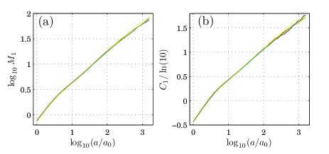
Figure 2: (a) $\log_{10}M_{1}$ and (b) $C_{1}/\ln(10)$ versus scale calculated by the increments method for five different couples $(F,L_{i})$ during fast crack growth.

Influence of force and initial length. On Fig. 2, we plot $\log_{10}M_{1}$ and $C_{1}/\ln(10)$ versus $\log_{10}(a/a_{0})$ for five different couples of values $(F,L_{i})$ during the fast growth stage. We see no dependence of $M_{1}$ and $C_{1}$ on the force or the initial crack size. The same independence is observed for the slow growth stage. These observations are independent of the definition chosen for $T[s](x,a)$ which means that our analysis is robust. In order to improve statistics, we will average the scaling laws obtained for data with different forces and initial crack lengths. We also notice that close to the discretization scale $a_{0}$ the slope becomes close to unity. This effect can be attributed to the discreteness of the signal Mitchell . In the following, we will concentrate on larger scales $a>4a_{0}$ ($\simeq$ maximum fiber diameter) where this effect can be neglected.

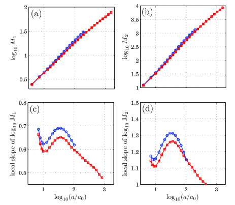
Figure 3: (a), (b): $M_{1}$ and $M_{2}$ for slow (circles) and fast (squares) crack growth. Statistical errors of the mean ($\equiv$ standard deviation $/\sqrt{N}$ with $N=102$) are smaller than symbol size. (c), (d): Corresponding local slope with an error comparable to the symbol size.

First and second order moments. Fig. 3(a) and (b) show log-log plots of $M_{1}$ and $M_{2}$ versus $a/a_{0}$ for slow and fast growth. The curves are slightly different for slow and fast crack growth. Another important observation is that they are not perfectly straight lines. To magnify the difference, we plot the local slope of those curves (estimated as the mean slope on a half-decade window) on Fig. 3(c) and (d). One can see an evolution of the slopes with scale, in a similar fashion for fast or slow cracks. However, we observe a systematic difference between the slope values which is almost independent of the scale but depends on the moment order. Also, assuming that the moments are approximately linear, it is not possible to conclude for a roughness exponent value since the typical slopes $\zeta(1)$ and $\zeta(2)$ are such that $\zeta(2)\neq 2\zeta(1)$.

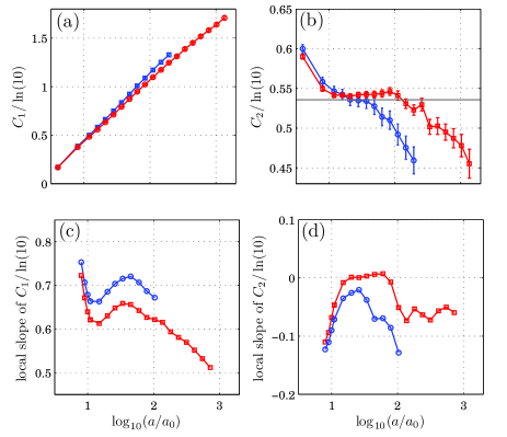
Figure 4: (a), (b): $C_{1}$ and $C_{2}$ versus scale with statistical error bars. In (b), the horizontal solid line corresponds to a signal with Gaussian statistics. (c), (d): Corresponding local slope of cumulants with an error comparable to the symbol size.

First and second order cumulants. On Fig. 4(a) and (b), we plot $C_{1}(a)$ and $C_{2}(a)$ divided by $\rm{ln}(10)$ versus $\rm{log}_{10}(a/a_{0})$ for slow and fast crack growth. $C_{1}(a)$ is almost linear, but has the same qualitative behavior than $M_{1}$ or $M_{2}$ when looking at the local slope (see Fig. 4(c)). We will note the local slope $c_{1}^{F}(a)$ for the fast regime and $c_{1}^{S}(a)$ for the slow one. The separation between fast and slow crack growth is clearer on $C_{1}$ than on $M_{1}$ and $M_{2}$, and the difference in local slopes $\Delta c_{1}(a)=c_{1}^{S}(a)-c_{1}^{F}(a)$ is also more regular. The local extremum observed for $a/a_{0}\simeq 10^{1.5}$ ($a\simeq 500\,\mu\rm{m}$) in Fig. 4(c) suggests the existence of a characteristic scale for both regimes. In contrast, $C_{2}(a)$ is hardly a linear function. We note that there is a range of scales ($10<a/a_{0}<10^{2}$) for which the value of $C_{2}$ is close to the theoretical value for a signal with Gaussian statistics (see also Santucci06 ). However, in this range, the values of the local slope can be non-zero, especially for the slow regime (see Fig. 4(d)).

Scaling laws. From the various plots, we can already conclude that it is not so easy to find a range of scales for which clear scaling laws are observed. For $a/a_{0}\lesssim 10$, the slope of $C_{1}(a)$ is changing a lot because we start to feel the discretization effect previously discussed Mitchell . We clearly see that for $a/a_{0}\gtrsim 10^{2}$, the slope of $C_{1}(a)$ is again changing significantly and seems to go towards $0.5$. This can be attributed to a change of statistics at large scales. Thus, if a scaling law exists, it is observed mainly at intermediate scales where a small oscillation of the local slope is observed. The same conclusion can be reached by looking at $C_{2}(a)$. At large scale, $C_{2}(a)$ decreases to values smaller than the Gaussian value that have no physical meaning. At small scales, $C_{2}$ is very sensitive to discretization effects. At intermediate scales ($10<a/a_{0}<10^{2}$), $C_{2}$ appears quasi-constant. If one tries to estimate the slope $c_{2}$, one finds that $c_{2}$ is very close to zero for the fast crack growth and between $-0.08$ and $-0.02$ for the slow part.

We notice that the extremum value of $c_{2}$ ($\sim-0.02$) observed at intermediate scales for slow crack growth is close to the one found in Bouchbinder06 where both regimes were mixed. It is still difficult to confirm multiscaling since $c_{2}$ can be considered constant only over a very small range of scales. Nevertheless, the non-zero values observed for $c_{2}$ are important to consider since they will lead to $\zeta(2)\neq 2\zeta(1)$. Indeed, stopping at the second order, Eq. (6) predicts: $\zeta(1)=c_{1}+c_{2}/2$, and $\zeta(2)=2(c_{1}+c_{2})$. Thus, $\zeta(1)$ and $\zeta(2)$ are both influenced by the mean value of the Hölder exponent and its variance. In order to give meaningful information about the scaling properties of the crack, it is best to estimate directly $c_{1}$ from $C_{1}$ since, in the case of scale invariant signals, $c_{1}=\langle h\rangle$.

Table 1: Scaling exponents $c_{1}(=\langle h\rangle$) for fast and slow crack growth, and their difference using various methods.

Method	Fast growth	Slow growth	Difference
SF	0.64 $\pm$ 0.02	0.70 $\pm$ 0.02	0.06 $\pm$ 0.01
CWT	0.65 $\pm$ 0.02	0.73 $\pm$ 0.02	0.07 $\pm$ 0.01
WTMM	0.64 $\pm$ 0.01	0.70 $\pm$ 0.02	0.06 $\pm$ 0.01

Scaling exponents. We have estimated the scaling exponents in the range of scales for which the scaling laws are reasonably good. We took $a/a_{0}=10$ for the lower cut-off value, and for the upper cut-off value the point where $C_{2}$ cross the Gaussian value ($a/a_{0}=10^{2}$ for fast cracks, $a/a_{0}=10^{1.7}$ for slow cracks). In this scale range, we measure the mean and standard deviation of $c_{1}^{F}$, $c_{1}^{S}$ and $\Delta c_{1}$. We show in Table 1 the mean values $\pm$ the standard deviation using various methods (SF: structure functions, CWT : Continuous Wavelet Transform Parisi and WTMM : Wavelet Transform Modulus Maxima Muzy using $1^{st}$ derivative of Gaussian). All methods give a difference between the two growth regimes. For instance, structure functions give a difference of $0.06\pm 0.01$ with a roughness exponent of $0.64\pm 0.02$ for the fast regime and $0.70\pm 0.02$ for the slow regime. Note that these values are consistent with the ones in the literature Menezes ; HorvathSalminen . The standard deviation is smaller on the difference than on the scaling exponents themselves due to the regular shift between local slopes seen on Fig. 4(c).

Conclusion. Whatever are the exact scaling properties of cracks in paper, we find that the roughness changes when the rupture mechanism goes from sub-critical to fast crack growth. A decrease of the roughness exponent due to dynamical instabilities was previously observed in the case of fast crack growth Boudet . It would be interesting to understand if the smaller roughness in the fast regime comes from a similar effect. Nevertheless, roughness in the slow regime is probably controlled more by the material disorder than by dynamical effects. There seems to be a characteristic scale $a\simeq 500\,\mu\rm{m}$ in both growth regimes where the local slope of moments or cumulants reach an extremum value. Whether this scale is related to some internal structure of paper, for instance the fiber length, is an open issue.

- (1) J. Delour, J. F. Muzy and A. Arneodo, Eur. Phys. J. B 23, 243 (2001).
- (2) B. B. Mandelbrot, D. E. Passoja and A. J. Paullay, Nature 308, 721 (1984); A. L. Barabási and H. E. Stanley, Fractal concepts in surface growth (University Press, Cambridge, 1995).
- (3) E. Bouchaud, G. Lapasset, and J. Planès, Eur. Phys. Lett. 13, 73 (1990); E. Bouchaud, J. Phys.: Condens. Matter 9, 4319 (1997); K. J. Måløy, A. Hansen, E. L. Hinrichsen, and S. Roux, Phys. Rev. Lett. 68, 213 (1992).
- (4) E. Bouchbinder, I. Procaccia, and S. Sela, Phys. Rev. Lett. 95, 255503 (2005); L. Ponson, D. Bonamy, and E. Bouchaud, Phys. Rev. Lett. 96, 035506 (2006).
- (5) I. L. Menezes-Sobrinho, M. S. Couto, and I. R. B. Ribeiro, Phys. Rev. E 71, 066121 (2005).
- (6) J. M. Lopez, M. A. Rodriguez, and C. Cuerno, Phys. Rev. E 56, 3993 (1997).
- (7) E. Bouchbinder, I. Procaccia, S. Santucci and L. Vanel, Phys. Rev. Lett. 96, 055509 (2006).
- (8) J. Schmittbuhl, and K. J. Måløy, Phys. Rev. Lett. 78, 3888 (1997); P. Daguier, B. Nghiem, E. Bouchaud, and F. Creuzet, Phys. Rev. Lett. 78, 1062 (1997); J. M. Boffa, C. Allain, R. Chertcoff, J.-P. Hulin, F. Plouraboué, and S. Roux, Eur. Phys. J. B 7, 179 (1999).
- (9) J.-F. Boudet, S. Ciliberto, and V. Steinberg, J. Phys. II 6, 1493 (1996).
- (10) M. J. Alava, P. K. V. V. Nukala, and S. Zapperi, Adv. in Phys. 55, 349 (2006).
- (11) V. Horvath, J. Kertész and F. Weber, Fractals 1, 67 (1993); L. I. Salminen, M. J. Alava, and K. J. Niskanen, Eur. Phys. J. B 32, 369 (2003).
- (12) J. Schmittbuhl, J.-P. Vilotte, and S. Roux, Phys. Rev. E 51, 131 (1995).
- (13) S. Santucci, L. Vanel, and S. Ciliberto, Phys. Rev. Lett. 93, 095055 (2004); S. Santucci et al., Europhys. Lett. 74, 595 (2006).
- (14) G. Parisi, and U. Frisch in Turbulence and Predictability in Geophysical Fluid Dynamics, ed. M. Ghil, R. Benzi and G. Parisi, North -Holland, Amsterdam, 84 (1985).
- (15) J. F. Muzy, E. Bacry and A. Arneodo, International J. Bifurcation and Chaos 4, 245 (1994).
- (16) S. Mallat, A Wavelet Tour of Signal Processing, Academic Press, Boston, (1997).
- (17) I. Simonsen and A. Hansen, Phys. Rev. E 58, 2779 (1998).
- (18) A. L. Barabási, R. Bourbonnais, M. H. Jensen, J. Kertész, T. Vicsek and Y. C. Zhang, Phys. Rev. A 45, R6951 (1992).
- (19) L. Chevillard, S.G. Roux, E. Leveque, et al., Phys. Rev. Lett. 91, 214502 (2003); 95, 064501 (2005).
- (20) S. J. Mitchell, Phys. Rev. E 72, 065103 (2005).
- (21) S. Santucci et al., cond-mat/0607372.