Nonlinear Diffusion Through Large Complex Networks Containing Regular Subgraphs

Abstract

Transport through generalized trees is considered. Trees contain the simple nodes and supernodes, either well-structured regular subgraphs or those with many triangles. We observe a superdiffusion for the highly connected nodes while it is Brownian for the rest of the nodes. Transport within a supernode is affected by the finite size effects vanishing as $N\to\infty.$ For the even dimensions of space, $d=2,4,6,\ldots$, the finite size effects break down the perturbation theory at small scales and can be regularized by using the heat-kernel expansion.

PACS codes: 87.15.Vv, 89.75.Hc, 89.75.Fb

Keywords: Structures and organization in complex systems, Networks and genealogical trees, Diffusion

1 Introduction

Complex networks have become a new paradigm in physics. They have been studied extensively due to their relevance to many real systems from the World Wide Web to the biological and social networks. Graph theory has been successfully applied to a wide range of different disciplines requiring a description of sets of elements either connected or interacting pairwise. Geometry and topology of underlying graphs have a deep influence on the physical properties of complex networks. In view of that one is interested in the properties of graphs which affect the dynamical behavior in the models defined on them. On the other hand, the study of large complex systems calls for the statistical methods, to give an effective description of collective dynamical behavior observed in them.

In the present paper, we study the nonlinear transport on large inhomogeneous graphs.

Diffusion processes defined on the 1-dimensional small world networks have been considered in [1]. It appears that the mean field theory breaks down for the small worlds models in dimensions $d<2$ [2] due to the emergence of strong site-to-site fluctuations of the Green’s functions. In [3], the $\epsilon$-expansion for a small world model has been developed where $\epsilon=2-d$ (quantifies the departure of the space dimension from $2$). The small world network is constructed by adding random shortcuts to a regular lattice, and the density of links $p>0$ has been taken enough small: $pa^{d}\ll 1$ where $a$ is the lattice scale. The Green’s functions have been computed for $d=2$, but the $\epsilon$-expansion breaks down for $\epsilon=1$ due to traps appearing in the system at $d=1$. In contrast to the small worlds model [3], we consider the diffusion processes defined on graphs approaching the networks known in the literature as ”froths” [4]; they could contain the regular subgraphs but are, in general, far from being the regular lattices. The space tiled by the froth can be curved, and, in such a case, the intrinsic dimension of the cellular system does not coincide with the dimension of the embedding space.

Transport phenomena had been extensively studied for the disordered media [5]-[7] and fractals [8]-[10]. It has been revealed that the transport properties depend upon the intrinsic dimension $d_{f}$ of disordered systems. In particular, the random walk probability $P$ is proportional to $t^{-d_{f}/2}f(x/\sqrt{t})$ where $f$ is a scaling function. Similar results have been reported for nonlinear diffusion processes [11]-[16].

In our model, we consider the complex networks as the generalized trees with two types of nodes: the simple nodes (more often of low connectivity) and the supernodes which are either the subgraphs containing many polygons or the $k$-regular subgraphs. In a continuous setting, the supernodes can be treated as complete compact curved Riemann surfaces characterized by the finite areas (see Sec. 3). The supernodes are bridged by the tree components. We study the large scale asymptotic behavior of nonlinear transport process defined on such the generalized trees. It is affected by both the space curvature within a supernode and the variation of space dimension between the supernodes.

Strictly speaking, the possibility to replace a finite graph by a compact continuous manifold for a nonlinear diffusion process is a challenging question. For the linear differential operators acting on the periodic functions, it requires that the spectra associated to the discrete and continuous problems are similar [17]. In particular, the multiplicities of the eigenvalues should be equal for both problems.

However, by this time, it is still not much known even about the spectral properties of Schrödinger operators defined on curved compact manifolds. Some estimations on the multiplicities of eigenvalues and the Euler characteristic of a surface can be found for the 2D-sphere, for the Klein’s bottle, and for the 2D-torus in [18]-[22]. Therefore, even in this case, the justification of the validity for the approximation of processes defined on the graphs by that ones defined on the compact continuous manifolds is a difficult problem. Concerning the nonlinear diffusion process, we should confess that such an approximation is always an assumption.

We consider the diffusion as a generalized Brownian motion with arbitrary boundary conditions described by a functional integral (see Sec. 4). The nonlinear term included into the diffusion equation models the effect of varying space dimension, the possible fluctuations of transport coefficient, the diffusion-reaction processes, and the possible queueing due to a bounded transport capacity of edges bridging the supernodes (see Sec. 5). The fluctuations have been treated in the framework of field theory approach.

The large scale asymptotic behavior of Green function is a superdiffusion for the nodes of high connectivity, while it is still Brownian for the rim nodes (see Sec. 6). In the regular subgraphs endowed with the standard orientation of edges, the effect of space ”curvature” within a supernode rises the finite size corrections to the scaling behavior (see Sec. 6 and Appendix A). In Sec. 7, we use the heat-kernel expansion to regularize the effective action functional at the small scales for the even dimensions of space $d=2,4,6,\ldots.$

2 Description of the model and the results

We are interested in the large scale asymptotic behavior of Green function for the diffusion equation for the density $u(x,t)$ defined on the curved Riemannian manifold with metric tensor $g_{ij}$, with the nonlinear term $\propto u^{\alpha}$ ($\alpha>1$) included. We assume the such a model can be considered as an approximation of nonlinear diffusion process defined on the graphs containing the large regular subgraphs. This approximation, however, is rather intuitive and cannot be proven nowadays rigorously. If the assumption is true, then $\log_{2}\mathrm{deg}(x)$ plays the role of effective local space dimension at node $x$ on the graph, $\mathrm{deg}(x)$ being the degree of $x$. The nonlinear diffusion term is relevant to the large scale asymptotic behavior if

$$\alpha\leq 1+\frac{2}{\log_{2}\textrm{deg}(x)}$$

and is irrelevant otherwise.

In the critical phenomena theory, the physical degrees of freedom are replaced by the scaling ones related to each other by the RG transformations. The large scale asymptotic behavior of physical system is then determined by the properties of scaling invariant system at a certain stable fixed point of the RG differential equation. The derived results are irrelevant to the order of space and time (infinite) limits.

Our main result is that for the large scale asymptote of Green function,

$$G(t)\sim\left\{\begin{array}[]{ll}t^{-\log_{2}\mathrm{deg}(x)/2},&\log_{2}\mathrm{deg}(x)>\frac{2}{\alpha-1},\quad x\in\Gamma,\\ t^{-1/\alpha-1},&\log_{2}\mathrm{deg}(x)\leq\frac{2}{\alpha-1},\quad x\in\Gamma,\end{array}\right.$$

The main technical difficulty of computations in the curved space metrics is the lack of the global frequency-momentum representation. In order to regularize the effective action at small scales in the one-loop order, we have used the heat-kernel expansion which does not depend upon the space-time topology. In the regular graphs endowed with the standard orientation of edges (the cycling ordering of edges to be the same for all nodes), the effect of curvature within the supernodes reveals itself by the finite size corrections to the scaling behavior.

3 The regular subgraphs viewed as Riemann surfaces

In the present paper, we consider the flat Euclidean space $\mathbb{R}^{d}$ as the limit $a\to 0$ of a regular lattice $\mathcal{L}_{a}=a\mathbb{Z}^{d}$ with lattice scale length $a$. For simulating the diffusion equation $u_{t}=\triangle u$ for the scalar function $u$ defined on the lattice, one uses its discrete representation,

$$u^{t+1}(x)=\frac{1}{2^{d}a^{2}}\left[\sum_{y\in U_{x}}u^{t}(y)-2^{d}u^{t}(x)\right],$$ (1)

where $U_{x}$ is the lattice neighborhood of $x\in\mathcal{L}_{a}$. The cardinal number $2^{d}$ is uniform for a given $\mathcal{L}_{a}$, and $d$ is interpreted as the dimension of Euclidean space.

Being defined on an arbitrary connected graph $\Gamma=(V_{\Gamma},E_{\Gamma}),$ in which $V_{\Gamma}$ is the set of its vertices and $E_{\Gamma}$ is the set of edges linking them, the discrete Laplace operator has actually the same form as in (1) excepting for the cardinality number changed to $2^{\delta_{x}}$ where $\delta_{x}=\log_{2}\mathrm{deg}(x)$ and $\mathrm{deg}(x)$ is the degree of vertex $x\in\Gamma$. By counting the number of vertices $|V_{\Gamma}|$, the number of edges $|E_{\Gamma}|$, and the number of faces $|F_{\Gamma}|$, one obtains the Euler characteristic of a planar graph $\Gamma$,

$$\chi(\Gamma)=|V_{\Gamma}|-|E_{\Gamma}|+|F_{\Gamma}|,$$

and its genus,

$$\mathrm{g}(\Gamma)=\frac{2-\chi(\Gamma)}{2},$$ (2)

the number of nonintersecting cycles on the graph $\Gamma$. We are interested in the subgraphs of $\Gamma$ ample with polygons, in particular, the triangles, which can be used as a base for a local mesh of a Riemann surface (the Delaunay triangulation).

An intuition on the deep relation between the triangle structures in the complex networks and their curvature has been expressed in [26]: ”Triangles capture transitivity, which we measure by the associated notion of curvature”. In [27], upper and lower bounds on the number of graphs of fixed degree which have a positive density of triangles have been estimated. In particular, it has been shown that the triangles seem to cluster even at low density. Then, in [28] it has been proven that the probability for a randomly selected vertex to participate in $T$ triangles decays with $T$ following a power-law, if the graph is scale free with the degree exponent satisfying $2<\beta<2.5$. Moreover, if $\beta=2+1/3$, the density of triangles appears to be finite in such graphs.

The Laplace-Beltrami operator on a triangle mesh has been defined in connection with the various graphical applications such as mesh fairing, smoothing, surface editing in $3D$-space [29]-[32]. The stiffness matrix correspondent to it can be computed for each triangle specified by its vertices $\mathbf{x}=(x_{1},x_{2},x_{3})$, $\mathbf{y}=(y_{1},y_{2},y_{3})$, $\mathbf{z}=(z_{1},z_{2},z_{3})$ as

$$\mathbf{K}=S_{\triangle}\mathbf{B}\mathbf{B}^{T},\quad\mathbf{B}=\frac{1}{2S_{\triangle}}\left(\begin{array}[]{ccc}x_{2}-x_{3}&y_{2}-y_{3}&z_{2}-z_{3}\\ x_{3}-x_{1}&y_{3}-y_{1}&z_{3}-z_{1}\\ x_{1}-x_{2}&y_{1}-y_{2}&z_{1}-z_{2}\end{array}\right)$$

where $S_{\triangle}$ is the area of triangle.

However, from the various models of complex networks, it seems rather easier to count the number of edges which link a node to others than to check out if its neighbors are really connected forming triangles. Instead of hunting for triangles, while analyzing the graphs of real world networks, one can search for the 3-regular subgraphs ${}_{3\mathrm{R}}\Gamma$ for which there are precisely three edges incident at each vertex (loops are counted twice, multiple edges are allowed). These graphs form a honeycomb. The idea of using 3-regular subgraphs to study the topological properties of rendered Riemann surfaces has been proposed in [33]. In [34, 35], it has been shown that for each 3-regular graph ${}_{3R}\Gamma$ of $2N$ nodes with an orientation $\mathcal{O}$ (which assigns to each vertex of ${}_{3R}\Gamma$ a cyclic ordering of edges incident at it) one can construct a complete Riemann surface $S({}_{3R}\Gamma,\mathcal{O})$ by associating the ideal hyperbolic triangles to each vertex of ${}_{3R}\Gamma$ and gluing sides together according to the edges of the graph ${}_{3R}\Gamma$ and the orientation $\mathcal{O}.$ The resulting surface is endowed with a metric excepting for the finitely many points (cusps) where the metric could be undefined. The surface area is finite and equals to $2\pi N$. The conformal compactification of $S({}_{3R}\Gamma,\mathcal{O})$ are dense in the space of Riemann surfaces. The standard orientation on the 3-regular graph which is the 1-skeleton of a cube contains six left-hand-turn paths on which a traveller always turns left, giving that the associated surface is a sphere with six punctures. The choice of different orientations can give surfaces of genus 0,1, and 2, [34].

The closed paths of length $k$ on ${}_{3\mathrm{R}}\Gamma$ are homotopic to the closed geodesic lines on $S(\Gamma,\mathcal{O})$. Their cardinality is defined by the spectral density of ${}_{3\mathrm{R}}\Gamma$-subgraph that is the density of eigenvalues of its adjacency matrix [23],

$$\varrho(\lambda)=\frac{1}{N}\sum_{j=1}\delta(\lambda-\lambda_{j}),$$

which converges to a continuous function with $N\to\infty$ ($\lambda_{j}$ is the $j-$th largest eigenvalue of adjacency matrix $\mathbf{A}$). The $k-$th moment $M_{k}$ of $\varrho(\lambda)$ scales with the number of cycles $C_{k}$ of length $k$,

$$M_{k}=\frac{1}{N}\sum_{j=1}^{N}\lambda_{j}^{k}=\frac{1}{N}\mathrm{Tr}(\mathbf{A}^{k})=\frac{k}{N}C_{k},$$

$C_{k}$ can be computed by using of the zeta-function,

$$\zeta(z)=\frac{1}{\det(\mathbf{1}-z\mathbf{A})}.$$

Namely,

$$C_{k}=\left.\frac{1}{(k-1)!}\frac{d^{k}}{dz^{k}}\zeta(z)\right|_{z=0}.$$

All roots of the polynomial $\det(\mathbf{1}-z\mathbf{A})$ lay on the unit circle and coincide with the inverse of the eigenvalues $\lambda_{j}^{-1}$ of adjacency matrix excepting for the zeros, $\{\lambda=0\}$. It is worth to mention that $S({}_{3R}\Gamma,\mathcal{O})$ allows for a conformal compactification, [34].

4 Model of nonlinear diffusion through complex networks

In the previous section, we have supposed that a regular subgraph in a complex network can be treated, in a continuous setting, as a Riemann space of finite area characterized by some metric tensor. For a particular time slice, the line element $ds$ between each pair of neighboring points on the spatial surface is given by

$$ds^{2}=\sum_{ij}g_{ij}(x)dx^{i}dx^{j}$$

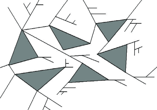
Figure 1: In the model, we consider the complex networks as the generalized trees with two types of nodes: the simple nodes (probably of low connectivity) and the supernodes which are either the subgraphs with many triangles or the $k$-regular subgraphs.

where $dx^{k}$ denote the differences between neighboring points, and $g_{ij}$ denotes the metric tensor. Then, the complex network as a whole can be considered as a disordered media in which the compact islands $S$ of curved Riemann space (with the ”effective” space dimensions $\delta_{S}$) are bridged by the tree like graph components (see Fig. 1) in which the local space dimension $\delta_{x}$ can vary from point to point.

The transport properties through such a disordered media is essentially of nonlinear nature. In the previous studies of nonlinear diffusion [11] -[16], the authors had introduced various nonlinear terms into the diffusion equation modelling the possible fluctuations of transport coefficient, the diffusion-reaction processes, and the queuing due to a bounded transport capacity of edges. We also introduce it for accounting the effect of varying dimension of space in the complex network (see the discussion below). To be certain, let us consider the equation for the scalar density field $u(\mathbf{x},t)$ defined on a Riemann surface,

$$\nabla_{t}u=g_{0}^{ij}\nu_{0}\frac{\partial^{2}u}{\partial x_{i}\partial x_{j}}-\xi_{0}\nu_{0}Ru-\eta_{0}\nu_{0}u^{\alpha},\quad\nabla_{t}\equiv\partial_{t}+b_{0}^{i}\frac{\partial}{\partial x_{i}}.$$ (3)

All $0$-subscripted variables denote their bare values before the application of the renormalization group transformation. In Eq. (3), the Riemann metric tensor $g_{0}^{ij}$ depends upon the chosen conformal parameterization of regular subgraphs, $R$ is the scalar curvature. We prefer to keep the entries of $g_{0}^{ij}$ dimensionless therefore we have introduced the parameter $\nu_{0}$ having the dimension of a viscosity. For the purpose of this paper, we will examine metric rescalings that are spacetime constants (we suppose that the subgraph of $\Gamma$ is regular and the edges do not rewire with time). However, it is possible to consider the effect of a rescaling given by a spacetime-dependent function.

The covariant derivative $\nabla_{t}$ contains the curvature drift term proportional to $b_{0}^{i}=g_{0}^{jk}\Gamma^{i}_{jk}$ (the curvature drift velocity) which expresses the local anisotropy of space because of its curvature. $\Gamma^{i}_{jk}$ are the Christoffel symbols calculated out from the metric tensor $g^{ij}$ in the standard way, $\Gamma^{i}_{jk}=g^{il}(g_{kl,j}+g_{jl,k}-g_{jk,l})/2$. While being interested in the long time large scale ranges, one usually keeps only the first order derivative term $\partial_{i}$ if it presents in the linear part of equation since its contribution $O(k)$ should dominate over the diffusion $O(k^{2})$ for small $k$. Nevertheless, we keep both terms to ensure the convergence of integrals in time, in the limit of flat metric. However, in the general curved spacetime, the homogeneity required for the existence of a global momentum space representation is lacking.

The real valued parameters $\xi_{0}$ and $\eta_{0}$ are the bare coupling constants governing the coupling of configurations $u$ to the scalar curvature of space $R$ and to the varying effective space dimensionality $\delta_{x}$ respectively. We assume them to be small. The nonlinearity exponent is $\alpha>1$ ($\alpha$ is not necessary integer) [11] -[16].

Let us explain the role played by the nonlinear term in (3) in more details. In the critical phenomena theory, the physical degrees of freedom are replaced by the scaling degrees of freedom. In particular, one considers the canonical dimension $d_{F}$ instead of time and space physical dimensions of the quantity $F$. The analysis of canonical dimensions allows for the selection of relevant interactions among all possible interaction which could arise in the model. In the spirit of critical phenomena theory, the nonlinear term that could affects substantially the large scale asymptotic behavior typical for the diffusion process should have the same canonical dimension as the normal diffusion. If the canonical dimension of the nonlinear term added to the equation is less than of the ordinary diffusion, it has to be neglected. The opposite is also true: if the nonlinear term provides the leading contribution to the asymptotic behavior, then the diffusion term has to be dropped.

Therefore, it is interesting to consider the model in which the nonlinear term would play an important role. Below, we demonstrate that the exponent $\alpha$ is related to the dimension of space $d$ and the dimension $[\eta_{0}]$ of coupling constant $\eta_{0}$. If we assume for a moment that in the vicinity of some point the dimension of space $d$ is changed to some other value $\delta$, then, strictly speaking, Eq. (3) could have no sense therein: either the diffusion term or the nonlinearity should be neglected. For given $\alpha$ and $[\eta_{0}]$, there is only one value $d$ at which the Eq. (3) is relevant with respect to the large scale asymptotic behavior of diffusion process. If we consider the plane of parameters $[\eta_{0}]$ and $\alpha$, then the relevant space dimensions $d$ is a line on it. Therefore, by tuning the values of $\alpha$ and $[\eta_{0}]$, one can ”modify” the space dimension $d$ in the model of nonlinear diffusion. It is indeed unphysical to change the nonlinearity exponent $\alpha$ (we suppose that $\alpha$ is a property of a certain physical process), however, one can tune the value of $[\eta_{0}]$ and use it as the small expansion parameter of perturbation theory (like the parameter $\varepsilon=4-d$ in the Wilson’s theory of critical phenomena).

A similar idea is used in the usual dimensional regularization of Feynman diagrams. In the continuous Euclidean space, the dimensional regularization scheme does not look natural and therefore is usually treated as a formal trick which helps to reformulate the singularities arisen in the Feynman graphs in the form of poles in $\varepsilon$. However, if the dimension of physical space could vary, than the dimensional regularization would acquire the natural meaning provided the nonlinearity exponent $\alpha$ is fixed and the correspondent nonlinear diffusion process is relevant with respect to the large scale asymptotic behavior.

As we have mentioned above, such a relevance can be justified by means of dimensional analysis [12, 16]. Dynamical models have two scales: the length scale $L$ and the time scale $T$. The physical dimension of viscosity is $[\nu_{0}]=L^{2}T^{-1},$ of the scalar curvature is $[R]=L^{-2}$, and of the drift velocity is $[b_{0}^{i}]=LT^{-1}$. Let us choose the physical dimension for the coupling constant to be $[\eta_{0}]=L^{-2\varepsilon}$ (assuming that $\varepsilon=0$ in the logarithmic theory when the nonlinear interaction is marginal) and note that the dimension of a scalar quantity is $[u]=L^{-d}.$ In the free theory, $\partial_{t}\propto\partial^{2}$ and in the analysis of canonical dimensions one has $L^{2}\sim T$. All terms in (3) should be of the same canonical dimension, in particular $[\partial_{t}u]=[\eta_{0}\nu_{0}u^{\alpha}]$, therefore $-2+\log_{L}[u]=\alpha\log_{L}[u]-2\varepsilon$ and finally, $[u]=L^{2(1-\varepsilon)/(1-\alpha)}$, from which it follows that

$$d=2\cdot\frac{1-\varepsilon}{1-\alpha}.$$ (4)

The above relation gives us a hint of that the space dimension in the model of a nonlinear diffusion can be effectively tuned by the parameters $\alpha$ and $\varepsilon.$ We choose the parameter $\varepsilon$ to quantify the local irregularity of the graph by measuring the relative deviation of the node degree $2^{\delta_{x}}$ from the cardinality number $2^{d}$ in the regular lattice,

$$\varepsilon=1-\frac{d}{\delta_{x}}.$$ (5)

The nodes with $\mathrm{deg}(x)<2^{d}$ correspond to $\varepsilon<0$, while the nodes for which $\mathrm{deg}(x)\geq 2^{d}$ are described by $\varepsilon\geq 0.$

We supply Eq. (3) with the locally integrable initial condition $u(\mathbf{x},0)$ and study the standard Cauchy problem being interested in the large scale asymptotic Green’s functions $G(\mathbf{x},\mathbf{x_{0}};t,t_{0}).$ For a curved space, the natural way to proceed is to examine the change to the Green’s functions as the metric is scaled. This can be achieved by moving the points along the geodesics (cycles in the graph $\Gamma$) connecting them or alternatively by scaling the geodesic distance function (the metric).

The Green’s functions of nonlinear problem (3) supplied with the integrable initial conditions can be formally calculated by the perturbation series with respect to the nonlinearity (as the coupling parameter $\eta_{0}$ is small) followed by the integrations over the initial condition $u(\mathbf{x},0).$ Some integrals estimating corrections to the linearized diffusion problem diverge logarithmically since the integration domain is not compact. If we introduce the $\varepsilon$-parameter in accordance to (5), the divergences reveal themselves by the poles in

$$\varepsilon=1+d\cdot\frac{1-\alpha}{2}.$$

Therefore, the nonlinear interaction is irrelevant (in the sense of Wilson) for $\varepsilon<0$ ($d>2/(\alpha-1)$), but is essential as $\varepsilon\geq 0$ when the ordinary perturbation expansion (in the form of series in $\eta_{0}$) fails to give the correct large scale asymptotic behavior and the whole series has to be summed up. For instance, it happens at $d=2$ for $\alpha=2$.

In other words, the logarithmic (marginal) value of $\alpha$ is determined by comparison of the nonlinear contribution with that of the linear dissipative term, $\alpha{\ }_{\mathrm{log}}=1+2/d$. While introducing the parameter $\varepsilon$ accounting for the local change of connectivity in the graph, we effectively pass from $\alpha{\ }_{\mathrm{log}}$ to its new value $\alpha{\ }^{\prime}_{\mathrm{log}}=1+2/\delta_{x}$. Then it turns that the nonlinear contribution to the long range asymptotic transport through the rims ($\varepsilon<0$) is irrelevant in comparison with the linear diffusion and therefore can be neglected. In contrast to it, the contribution coming from hubs ($\varepsilon\geq 0$) is more essential than the linear one and has to be taken into account in all orders of perturbation theory since the relevant fluctuations dominate the diffusion at large scales.

We calculate the asymptotic Green’s functions for the model (3) in the logarithmic theory (on the regular subgraphs with the cardinality number $2^{d}$) in curved space metric and develop the $\varepsilon-$expansion accounting for the corrections in the long time large scale region due to the irregularity of graph. The relevant contributions to the nonlinear transport coming from hubs are summed by the field-theoretic renormalization group method. Herewith, the real values of parameter $\varepsilon$ has to be taken as $\varepsilon_{x}=1-{d}/{\delta_{x}},$ the excess of hub’s connectivity over the regular cardinality number $2^{d}$.

We conclude this section by remarking that the problem of renormalization in a curved spacetime has been discussed extensively in the literature ([37]-[45] and by other authors). However, it has never been studied in connection with the critical phenomena theory. The analysis of transport through the graphs would provide us with such a model. It is worth to mention that in contrast to the case of the gravitational field, we are not restricted on graphs by the equivalence principle, so that the curved space has not to be flattened in any sufficiently small region.

5 Diffusion as a generalized Brownian motion

We set up a field theory formalism for the study of asymptotic properties of the Green’s function by means of the renormalization group (RG) equations which are valid in the curved spaces. Our method is closely related to the approach discussed in [38] regarding the Green’s functions as the functions of metric and scaling the metric instead of scaling the coordinates or moments.

It is well known that many problems of stochastic dynamics (and of the transport through a disordered media, in particular) can be treated as a generalized Brownian motion, $P(u)={\left\langle{\delta\left({u-u\left({\mathbf{x},t}\right)}\right)}\right\rangle},$ in which the average is taken over all configurations of field $u(\mathbf{x},t)$ satisfying the dynamical equation

$$\nabla_{t}u-\nu_{0}\Delta_{LB}u+\nu_{0}\eta_{0}u^{\alpha}+\xi_{0}\nu_{0}Ru=\frac{1}{\sqrt{g}}\delta(t-t_{0})\delta(\mathbf{x}-\mathbf{x}_{0}),$$ (6)

for the integrable initial condition $u(\mathbf{x},0)$ and arbitrary conditions on the boundaries of the graph. The Laplace-Beltrami operator $\Delta_{LB}$ is given by (3), and $g=|\det g_{0}^{ij}|.$

We use the functional representation of the $\delta-$function for expressing the probability,

$$P(u)=\int\mathcal{D}u\int\mathcal{D}u^{\prime}\exp\left(u^{\prime}\left(u-u(\mathbf{x},t)\right)\right),$$ (7)

in which $u$ marks the position of a ”particle”, and the auxiliary field $u^{\prime}$ (of the same nature as $u$) is not inherent to the original model, but appears since we treat the dynamics as a Brownian motion. The formal convergence requires the field $u$ to be real and the field ${u}^{\prime}$ to be purely imaginary. Should a unique solution of dynamic equation exists, we perform the natural change of variables in (7),

$$\left(u-u(\mathbf{x},t)\right)\to-\nabla_{t}u+\nu_{0}\Delta_{LB}u-\nu_{0}\eta_{0}u^{\alpha}-\xi_{0}\nu_{0}Ru-\frac{1}{\sqrt{g}}\delta(t-t_{0})\delta(\mathbf{x}-\mathbf{x}_{0})=0,$$

from which it follows that

$$P(u)=\int\mathcal{D}u\int\mathcal{D}u^{\prime}\exp\mathcal{S}(u,u^{\prime})\det\mathbf{M}$$

where $\det\mathbf{M}$ is the Jacobian associated to the change of variable, and $\mathcal{S}(u,u^{\prime}),$ the action functional,

$$\mathcal{S}=\mathcal{S}_{0}-\eta_{0}\nu_{0}\mathrm{Tr}_{g}(u^{\prime}u^{\alpha})-\frac{1}{\sqrt{g}}u^{\prime}(\mathbf{x}_{0},t_{0}),\quad\mathcal{S}_{0}=\mathrm{Tr}_{g}\left(-u^{\prime}\nabla_{t}u+\nu_{0}u^{\prime}\Delta_{LB}u-\xi_{0}\nu_{0}Ru^{\prime}u\right).$$ (8)

The trace $\mathrm{Tr}_{g}$ means the summation over the discrete indices and the integration $\int dv_{x}\int dt$ over the invariant volume element on the $d$-dimensional manifold, $dv_{x}=\sqrt{g(x)}d^{d}x.$

The Jacobian $\det\mathbf{M}$ deserves a thorough consideration. The linear part of the variable transformation can be factorized from it,

$$\det\mathbf{M}=\det\mathbf{M}_{0}\det(1-\Delta_{uu^{\prime}}\mathbf{M}_{1})$$ (9)

where $\mathbf{M}_{0}=-\nabla_{t}+\nu_{0}\Delta_{LB}-\xi_{0}\nu_{0}R$, the interaction part $\mathbf{M}_{1}=\alpha\nu_{0}\eta_{0}u^{\alpha-1}\delta(t-t^{\prime})$, and $\Delta_{uu^{\prime}}$ is the Feynman propagator in curved Riemann space, [46, 47], defined as the solution of linearized problem

$$(-\nabla_{t}+\nu_{0}\Delta_{LB}-\xi_{0}\nu_{0}R)\Delta_{uu^{\prime}}(\mathbf{x}-\mathbf{x}^{\prime},t-t^{\prime})=\frac{1}{\sqrt{g}}\delta(t-t^{\prime})\delta(\mathbf{x}-\mathbf{x}^{\prime}).$$

For more details as well as its explicit form see Appendix A.

It is important for us that the propagator $\Delta_{uu^{\prime}}$ is proportional to the Heaviside function $\theta(t-t^{\prime})$ as a consequence of causality principle. The first factor in (9) does not depend upon fields and therefore can be scaled out of the functional integration. The second factor in (9) can be expanded into the ”diagram” series,

$$\log\det(1-\Delta_{uu^{\prime}}\mathbf{M}_{1})=-\mathrm{Tr}_{g}(\Delta_{uu^{\prime}}\mathbf{M}_{1}+\frac{1}{2}\Delta_{uu^{\prime}}\mathbf{M}_{1}\Delta_{uu^{\prime}}\mathbf{M}_{1}+\ldots)$$

comprising of cycles of retarded Feynman propagators proportional to the Heaviside functions and therefore being trivial, excepting for the very first term, $\mathrm{Tr}_{g}(\Delta_{uu^{\prime}}\mathbf{M}_{1})$, in which the operator $\mathbf{M}_{1}$ contains $\delta(t-t^{\prime})$. The first term in the expansion is proportional to the undefined quantity $\theta(0)$ which value is usually taken as $1/2$. However, in the critical dynamics, another convention is used [48], $\theta(0)=0$ , under which the Jacobian $\det\mathbf{M}$ turns to be just a constant and therefore may be scaled out away at the irrelevant cost of changing only the normalization.

The action functional of type (8) in the problem of nonlinear diffusion in the flat metric has been introduced in [16]. In [49], the functional with an ultra-local interaction term like in (8) has been derived as a limiting one in the framework of MSR formalism (stochastic quantization, [50]). The renormalization of field theoretic models with ultralocal terms, located on surfaces, had been studied in [51] in details.

Further insight into the field theory representation of Brownian motion and the properties of auxiliary field $u^{\prime}$ can be obtained from the equations for the saddle-point configurations. The first equation, $\delta\mathcal{S}/\delta u^{\prime}=0,$ recovers the original Cauchy problem. The other one, $\delta\mathcal{S}/\delta u=0,$ reads as following

$$\nabla_{t}u^{\prime}+\nu_{0}\Delta_{LB}u^{\prime}-\xi_{0}\nu_{0}R=\alpha\eta_{0}\nu_{0}u^{\prime}u^{\alpha}$$

and is characterized by a negative viscosity. One can conclude from it that the auxiliary field should be trivial for positive time, $u^{\prime}(t>0)=0$, and decays as $t\to-\infty$.

In the framework of field theory approach, the Green function $G(x,t;x_{0},t_{0})$ for the Cauchy problem (6) can be computed as the functional average,

$$G(x,t;x_{0},t_{0})={\left\langle{u}\right\rangle}={\frac{{\int\mathcal{D}u\int\mathcal{D}u^{\prime}{u(x,t)\exp S(u,u^{\prime})}}}{{\int\mathcal{D}u\int\mathcal{D}u^{\prime}{\exp\left({S_{0}}\right)}}}},$$ (10)

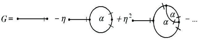
Figure 2: Three diagrams of the Feynman diagram expansion for the Green function of the nonlinear diffusion equation.

in which $\mathcal{S}$ is the action functional (8). The Green function (10) and all higher moments of fields $u$ and $u^{\prime}$ allow for the standard Feynman diagram series expansions. The diagram technique with the ultralocal interaction terms has been discussed in [16]. A special feature of such diagrams is that the final point of any diagram corresponds to $(\mathbf{x}_{0},t_{0})$. It is worth to mention that diagrams could formally contain a non-integer number of lines (since the nonlinearity exponent could deviate from an integer number). Diagrams are drawn of three elements: i) the final point $(\mathbf{x}_{0},t_{0})$ with an arbitrary number of attached $u^{\prime}$-legs (we mark them by a slash, see Fig.2); ii) the interaction vertex with one $u^{\prime}$-leg and $\alpha$ $u$-legs attached to it (we put the letter $\alpha$ inside the loop to stress that it is not necessarily integer); iii) the propagator $\Delta_{uu^{\prime}}$ is only available. The first three diagrams for the Green function (10) are sketched in Fig. 2.

6 Renormalization Group equation and scaling behavior of scalar field coupled to a complex network

Power-counting arguments [16] show that the divergent Feynman diagrams are those which involve any number of external $u^{\prime}$-legs (lines with slashes). For all these functions the formal index of divergence equals to zero, therefore all divergent contributions are logarithmic (the correspondent counterterms are constants). It is worth to mention that the model is renormalizable despite the fact that it requires an infinite number of counterterms. It is sufficient to renormalize the only ”one-particle-irreducible” Green function (the only diagram block which can be drawn using the elements i) - iii) mentioned above) to render the model finite.

Moreover, the counterterm corresponding to this block is sufficient to regularize all higher moments of fields $u$ and $u^{\prime}$, since any diagram of perturbation series is expressed as a convolution of equivalent blocks. Diagrams contain no additional superficial divergences [16]. We recall that all loops which could arise in the diagram expansions are created by the single local vortex with any number of $u^{\prime}-$legs incident at it. The counterterm corresponding to the elementary divergent block is constant and local in configuration space, i.e. $\propto\delta(t-t_{0})\delta(\mathbf{x}-\mathbf{x}_{0})$. In the action functional (8), the same local term appears, so that the model is renormalized multiplicatively, and only the renormalization constant $Z$ is required. To keep the interaction coupling constant $\eta$ dimensionless, one must introduce a mass parameter $\mu$.

The bare parameters are related to the renormalized parameters by

$$\nu_{0}=\nu,\quad\xi=\xi_{0},$$

$$\quad\eta_{0}=\eta\mu^{2\varepsilon}Z^{\alpha-1}.$$ (11)

The auxiliary fields and the Green function are related to their renormalized analogs by:

$$u^{\prime}=u^{\prime}_{R}Z,\quad G(\nu_{0},\xi_{0},\eta_{0})=Z^{-1}G_{R}(\nu,\xi,\eta,\mu).$$

The only renormalization constant required in the model is

$$Z=1+\sum_{l=1}\frac{c_{l}(\xi,\eta,\mu)}{\varepsilon^{l}}$$ (12)

where the amplitudes $c_{l}$ are defined to be precisely those needed to subtract the poles in the corresponding Feynman integrals. The derivation of the RG equation is carried through in a standard way since the curvature coupling parameter $\xi$ is not renormalized. We apply the standard RG differential operator $\mu\partial_{\mu}$ (for fixed $\nu_{0}$, $\eta_{0}$, $\xi_{0}$) to $G_{R}$ to obtain

$$\left[\mu\frac{\partial}{\partial\mu}+\mu\frac{\partial\eta}{\partial\mu}\frac{\partial}{\partial\eta}-\mu\frac{\partial}{\partial\mu}\ln Z\right]G_{R}(\nu,\mu,\xi,\eta)=0.$$ (13)

It follows from the relation (11) that for the RG functions (the coefficients in the RG equation) one has

$$\gamma(\eta)=\mu\frac{\partial}{\partial\mu}\ln Z,\quad\beta(\eta)=\eta\left(-2\varepsilon-(\alpha-1)\gamma(\eta)\right).$$ (14)

In the forthcoming section, we discuss the existence of a fixed point of RG transformation stable with respect to the long time large scale asymptotic behavior, that is a solution $\eta_{*}$ of equation $\beta(\eta)=0$ such that $\beta^{\prime}(\eta_{*})>0$ in the physical range of parameter $\eta>0$.

In the equation of critical scaling for the curved space, one has to take into account the new mass parameter $\varpi$ in addition to $\eta,$ $\xi$, and $\mu$. It had been introduced in [38] to quantify the dilatation $\varpi^{-1}g_{ij}$ of the background metric $g_{ij}$. The derivation of the scaling equation is standard: the canonical scale invariance of the renormalized Green function $G_{R}(\xi,\mu,\nu,\eta)$ with respect to dilatations of all variables is expressed by the equations

$$\left[\mu\frac{\partial}{\partial\mu}+\varpi\frac{\varpi}{\partial\varpi}-2\nu\frac{\partial}{\partial\nu}-x\frac{\partial}{\partial x}-d\right]G_{R}(\xi,\mu,\nu,\eta)=0,$$ (15)

$$\left[-t\frac{\partial}{\partial t}+\nu\frac{\partial}{\partial\nu}\right]G_{R}(\xi,\mu,\nu,\eta)=0.$$

In the IR fixed point of RG-transformation, one excludes the differential operations $\mu\partial_{\mu}$ and $\nu\partial_{\nu}$ using the RG equation (13) to obtain the equation of critical scaling,

$$\left[-\varpi\frac{\varpi}{\partial\varpi}+d-\gamma\right]G_{R}(\xi,\mu,\nu,\eta)=0,$$ (16)

where $\varpi$ is now interpreted as the metric scaling variable. If a stable point of RG transformation relevant to the long range asymptotical behavior $\eta_{*}$ exists in the model, the value of the anomalous dimension $\gamma$ at the fixed point is found exactly, owing to the relation between $\beta$ and $\gamma$,

$$\gamma_{*}=\gamma(\eta_{*})=-\frac{2\varepsilon}{\alpha-1}=-\frac{2}{\alpha-1}\left.\left(1-\frac{\delta_{x}}{d}\right)\right|_{\alpha=\alpha{}_{\log}}=\delta_{x}-d.$$ (17)

In agreement to dimensional considerations, the renormalized Green function has the form

$$G_{R}(t,r)=(\nu t)^{-d/2}\chi\left(\frac{r^{2}}{\nu t},\varpi\nu t,\frac{1}{t\mu^{2}\nu}\right),\quad r=|\mathbf{x}-\mathbf{x}^{\prime}|,$$

where $\chi$ is a scaling function of the dimensionless variables. The dependence on $\eta$ is not displayed explicitly, because the derivatives with respect to this parameter do not enter into the scaling equation. It follows from (16) that at the fixed point $\chi$ satisfies the equation

$$\left[z\frac{\partial}{\partial z}-\frac{\gamma_{*}}{2}\right]\chi(s,y,z)=0,$$

its general solution is $\chi(s,y,z)=s^{\gamma_{*}/2}\psi(s,y)$ where $\psi$ is an arbitrary function of the first and second arguments. For the Green function (10) we then obtain

$$G(t,r)\sim t^{-d/2-\gamma_{*}/2}\psi\left(\frac{r^{2}}{\nu t},\varpi\nu t\right)=t^{-\delta_{x}/2}\psi\left(\frac{r^{2}}{\nu t},\varpi\nu t\right),\quad\delta_{x}>d,$$ (18)

where the form of the scaling function $\psi$ is not determined by the equation (16). Although the value of $\gamma_{*}$ in (17) and the solution (18) have been obtained without calculation of the constant $Z$, such a calculation is necessary to check the existence and stability of the fixed point. Within the $\varepsilon-$expansion these facts can be verified already in the one-loop order. We perform it in the forthcoming section.

We conclude the section with a remark on the arguments of scaling function $\psi$ for the planar 3-regular graphs of order $2N$ with the standard orientation (i.e. the $2N$-honeycomb). In the Sec. 2, we have mentioned that they are equivalent to the sphere of radius $\rho$. The surface area of the sphere equals to $2\pi N=4\pi\rho^{2},$ and therefore $\rho=\sqrt{N/2}.$ The relevant Gilkey coefficients and the asymptotic behavior of the Feynman propagator as $t\to 0$ are given at the end of Appendix A. One can see that the corrections to the standard diffusion kernel risen by the space curvature can be naturally interpreted as the corrections due to the finite size of the 3-regular subgraph. Then, the scaling function $\psi$ is

$$\psi=\psi\left(\frac{r^{2}}{\nu t},\frac{2\nu t}{N}\right),$$

and it can be calculated by means of diagram expansion. In the thermodynamic limit, $N\to\infty,$ (when the the graph $\Gamma$ is large and regular) these corrections vanish and the scaling function depends only on one argument $r^{2}/\nu t$ relevant to the flat space. The result on the critical scaling (18) is still valid in the thermodynamic limit.

7 A fixed point of RG transformation and heat-kernel expansion

The main technical difficulty concerning diagram computations in curved spacetime is the lack of a global momentum-frequency representation. The momentum space is associated to each point $x^{\prime}$ by the Fourier transformation

$$f(x,x^{\prime})=\int\frac{d^{d}x}{(2\pi)^{d}}e^{iky}F(k;x^{\prime})$$

where $ky=g^{ij}k_{i}y_{j}$ which does not help much in calculations. In the flat metric, the calculation of the residue $c_{1}$ in (12), in the one-loop order, can be performed in the standard way using the momentum-frequency representation [16],

$$\left.c_{1}\right|_{\mathrm{flat}}=\frac{\eta\nu}{4\pi}\alpha^{-1/(\alpha-1)},\quad Z=1+\frac{c_{1}}{\varepsilon}.$$ (19)

It corresponds to the fixed point

$$\left.\eta_{*}\right|_{\mathrm{flat}}=\frac{\varepsilon}{\nu(\alpha-1)}$$ (20)

which is positive and stable for small $\varepsilon>0$ and $\alpha>1$. In the curved space the new singularities would arise at small scales (as $\mathbf{x}\to\mathbf{x}^{\prime}$) even for the metrics of constant curvature. They do not affect the renormalization group procedure (at least at the one-loop order) at large scales, but breaks down the perturbation theory for the even space dimensions.

The necessary regularization of effective action can be performed by using the heat-kernel expansion which does not depend on the spacetime topology (see, for instance, [39]). We consider the operator $Q_{2}$ with the kernel

$$Q_{2}=-\frac{\delta^{2}\mathcal{S_{R}}}{\delta U{\ }\delta V},\quad U,V=u,u^{\prime},$$

where $\mathcal{S}_{R}$ is the renormalized action functional of the model we consider. The one-loop amendment to the renormalized action is given by

$$L_{1}=-\frac{1}{2}\mathrm{Tr}\ln\left(Q_{2}\mathbf{\Delta}^{-1}\right)$$ (21)

where the propagator matrix is given by

$$\mathbf{\Delta}=\left(\begin{array}[]{cc}0&\Delta_{uu^{\prime}}\\ \Delta_{u^{\prime}u}&0\end{array}\right).$$

The counterterm corresponding to the only divergent diagram block is linear in the auxiliary field $u^{\prime}$. Variation of $L_{1}$ with respect to the auxiliary field

$$\delta_{u^{\prime}}L_{1}=\frac{1}{2}\mathrm{Tr}\left(\mathbf{\Delta}Q^{-1}_{2}\delta_{u^{\prime}}(Q_{2}\mathbf{\Delta}^{-1})\right),\quad\delta_{u^{\prime}}(Q_{2}\mathbf{\Delta}^{-1})=-\alpha(\alpha-1)\eta\nu u^{\alpha-2}\mathbf{\Delta}^{-1},$$

can be written as

$$\delta_{u^{\prime}}L_{1}=-\frac{1}{2}\delta_{u^{\prime}}\left\{\mathrm{Tr}\int_{0}^{\infty}\frac{d\tau}{\tau}\exp(-\tau\cdot Q_{2}\mathbf{\Delta}^{-1})\right\}.$$

Let us suppose that $\Lambda(t,\mathbf{x},\mathbf{y},Q_{2}{\mathbf{\Delta}}^{-1})$ is the kernel associated with the operator $\exp(-\tau\cdot Q_{2}{\mathbf{\Delta}}^{-1})$. Then, the one-loop contribution (21) reads as

$$L_{1}=-\frac{1}{2}\int dv_{x}\int^{\infty}_{0}\frac{d\tau}{\tau}\Lambda(\tau,\mathbf{x},\mathbf{x},Q_{2}{\mathbf{\Delta}}^{-1}).$$ (22)

Since the divergences are purely logarithmic, one can neglect the inhomogeneity of the scalar field $u$ in $\mathbf{x}$ while calculating the relevant counterterm. Being treated as a constant, the scalar $u$ renormalizes the scalar curvature,

$$R\to R-\frac{\alpha\nu\eta}{\xi}u^{\alpha-1},$$

so that one can define the modified Feynman propagator, $\Delta_{uu^{\prime}}\to\Delta_{uu^{\prime}}^{\prime}$.

Then, it appears that the kernel $\Lambda(\tau,\mathbf{x},\mathbf{x},(\mathbf{\Delta}^{\prime})^{-1})$ meets the ”heat equation”

$$[\partial_{\tau}+(\mathbf{\Delta}^{\prime})^{-1}]\Lambda(\tau,\mathbf{x},\mathbf{x},(\mathbf{\Delta}^{\prime})^{-1})=0$$

and therefore allows for the asymptotic expansion as $\tau\to 0+$, in the limit $\mathbf{x}\to\mathbf{x}^{\prime},$

$$\Lambda(\tau,\mathbf{x},\mathbf{x},Q_{2}{\mathbf{\Delta}}^{-1})\sim(4\pi\tau)^{-d/2}\sum_{m=0}^{\infty}\tau^{m}E_{m}(\mathbf{x},\mathbf{\Delta}^{\prime}),$$ (23)

in which $E_{m}(\mathbf{x},\mathbf{\Delta}^{\prime})$ are the relevant Gilkey coefficients [40]-[43]. In the case of a constant curvature metric, the first coefficients can be found in the Appendix A (27). Substituting the expansion (23) into the integral representation (22), one can perform the integrations with respect to the parameter $\tau$ with a cut off $\tau_{0}$. As a result, one arrives at the power series,

$$-\frac{1}{(4\pi)^{d/2}}\sum_{m=0}^{\infty}\frac{\tau_{0}^{m-d/2}}{m-d/2}E_{m}(\mathbf{x},\mathbf{\Delta}^{\prime}),$$ (24)

being singular for integer $m$ such that $d=2m$. It is obvious that the breakdowns of perturbation theory at small scales would happen for the even space dimensions. Extracting the pole part of $L_{1}$ one finds that

$$P.P.[L_{1}]=\frac{1}{(\delta_{x}-d)}\frac{1}{(4\pi)^{d/2}}\int dv_{x}E_{d/2}(x)=\frac{1}{\varepsilon}\frac{\delta_{x}}{(4\pi)^{d/2}}\int dv_{x}E_{d/2}(x)$$ (25)

where $E_{d/2}$ are the relevant Gilkey coefficient provided that $d$ is even. It is important to mention that in (25) the singularity coincides with that of (19). The residue in (25) has the ”good” signature and does not break the stability of the fixed point of RG transformation.

8 Discussion and Conclusion

In the present paper, we have studied the transport through the large complex networks containing regular subgraphs. We have considered such networks as generalized trees in which two types of nodes are allowed: simple nodes and supernodes. We have supposed that the supernodes are either the subgraphs with many polygons or $k$-regular subgraphs. In particular, we have discussed the case of 3-regular subgraphs which can be treated as the complete Riemann curved surfaces characterized by finite areas and can be compactified.

The diffusion process taking place on such a complex network is considered as a generalized Brownian motion with arbitrary boundary conditions. Its random dynamics is then described by a functional integral. We have studied the long time large scale asymptotic behavior of the Green function for the nonlinear diffusion equation defined on the complex network supplied with an integrable initial condition. The transport trough the complex network is of a strongly nonlinear nature being affected by both the varying effective space dimension between supernodes and the space curvature within a supernode.

In the regular graphs endowed with the standard orientation of edges (the cyclic ordering of edges to be the same for all nodes), the effect of curvature within the supernodes reveals itself by the finite size corrections to the scaling behavior. In the space of even dimensions , the curvature results in the additional singularities of Green function at small scales and calls for the special regularization. We have to stress that in contrast to the case of gravitational field, we are not restricted by the equivalence principle while considering models of complex networks. The main technical difficulty of computations in the curved space metrics is the lack of the global frequency- momentum representation. We have used the heat-kernel expansion which does not depend on the space time topology to regularize the effective action at small scales in the one-loop order.

Our approach to the complex networks containing large well-structured regular subgraphs could be used in studies of spreading of viruses [52] or social epidemics [53], traffic properties and the modelling of various ecological webs.

9 Acknowledgements

One of the authors (D.V.) benefits from a scholarship of the Alexander von Humboldt Foundation (Germany) and of a support of the DFG-International Graduate School ”Stochastic and real-world problems” that he gratefully acknowledges.

Appendix A. Feynman propagator in curved space

We present the explicit solution of the linearized diffusion problem, in the $d$-dimensional curved space metric, for $G(\mathbf{x},\mathbf{x}^{\prime},t)$ satisfying $\lim_{\mathbf{x}^{\prime}\to 0}G(\mathbf{x},\mathbf{x}^{\prime},t)=G(\mathbf{x},t)$ and $\lim_{t\to 0}G(\mathbf{x},\mathbf{x}^{\prime},t)=\delta(\mathbf{x}-\mathbf{x}^{\prime})$. The details can be found in [46] for field theories and in [47] (see also references therein) for classical models.

The general solution is

$$\Delta_{uu^{\prime}}(\mathbf{x},\mathbf{x}^{\prime},t)=\theta(t)\frac{\exp(-\xi_{0}\eta_{0}Rt)}{(4\pi t)^{d/2}}\exp\left(-\frac{\sigma(\mathbf{x},\mathbf{x}^{\prime})}{2t}\right)\Delta^{1/2}(\mathbf{x},\mathbf{x}^{\prime})\Omega(\mathbf{x},\mathbf{x}^{\prime},t)$$ (26)

where $\theta(t)$ is the Heaviside function, $\sigma(\mathbf{x},\mathbf{x}^{\prime})$ equals to half the square of the geodesic distance between $\mathbf{x}$ and $\mathbf{x}^{\prime}$, and $\Delta(\mathbf{x},\mathbf{x}^{\prime})$ is the van Vleck determinant,

$$\Delta(\mathbf{x},\mathbf{x}^{\prime})=-\frac{\det\left(\partial_{i}\partial_{j}\sigma(\mathbf{x},\mathbf{x}^{\prime})\right)}{\sqrt{g(\mathbf{x})g(\mathbf{x}^{\prime})}},$$

which reduces to unity in flat space, $R$ is the scalar curvature. The function $\Omega(\mathbf{x},\mathbf{x}^{\prime},t)$ allows for the following series expansion in the limit $\mathbf{x}^{\prime}\to\mathbf{x}$:

$$\lim_{\mathbf{x}^{\prime}\to\mathbf{x}}\Omega(\mathbf{x},\mathbf{x}^{\prime},t)=1+\sum_{l=1}^{\infty}t^{l}E_{l}(\mathbf{x})$$

valid in the limit $t\to 0$ where $E_{l}(\mathbf{x})$ are known in the literature as Gilkey coefficients [40]-[43]. For the diffusion equation, in the flat metric, the only coefficient which contributes is $E_{0}$ and we recover the well known standard diffusion kernel.

The planar 3-regular graph of order $2N$ with the standard orientation (the cyclic ordering of edges is taken the same for each node), a $2N$-honeycomb, corresponds to a sphere of radius $\rho=\sqrt{N/2}.$ The Ricci scalar curvature is then

$$R=\frac{2}{\rho^{2}}=\frac{4}{N},$$

and the Gaussian curvature equals to $\kappa=2/N.$ The Gilkey coefficients reduces to

$$E_{0}=1,\quad E_{1}=\frac{2}{3N},$$

$$E_{2}=\frac{4}{15}\frac{1}{N^{2}},\quad E_{3}=\frac{32}{315}\frac{1}{N^{3}}.$$ (27)

Then, in the limit $\mathbf{x}^{\prime}\to\mathbf{x}$ and $t\to 0$, the Feynman propagator exhibits the following dependence on the size of 3-regular subgraph:

$$\Delta_{uu^{\prime}}(\mathbf{x},t)=\theta(t)\frac{\exp\left(-\frac{x^{2}}{4\nu_{0}t}\right)}{4\pi\nu_{0}t}\left(1+\frac{1}{3}\left(\frac{2\nu_{0}t}{N}\right)+\frac{1}{15}\left(\frac{2\nu_{0}t}{N}\right)^{2}+\frac{4}{315}\left(\frac{2\nu_{0}t}{N}\right)^{3}+\ldots\right).$$ (28)

References

- [1] R. Monason, Eur. Phys. J. B 12, 555 (1999).
- [2] B. Kozma, M.B. Hastings, G. Korniss, Phys. Rev. Lett. 98 (10), 108701 (2004).
- [3] M. B. Hastings, Eur. Phys. Jour. B 42, 297 (2004).
- [4] T. Aste, Random walk on disordered networks , oai:arXiv.org:cond-mat/9612062 (2006-06-17).
- [5] Y. Limoge, J.L. Bocquet, Phys. Rev. Lett. 65, 60 (1990).
- [6] D. H. Zanette, P.A. Alemany, Phys. Rev. Lett. 75, 366 (1995)
- [7] M.U. Vera, D.J. Durian Phys. Rev. E 53, 3215 (1996).
- [8] S. Boettcher, M. Moshe, Phys. Rev. Lett. 74, 2410 (1995)
- [9] C.M. Bender, S. Boettcher, P.N. Meisinger, Phys. Rev. Lett. 75, 3210 (1995).
- [10] D. Cassi, S. Regina, Phys. Rev. Lett. 76, 2914 (1996).
- [11] N. Goldenfeld, O. Martin, Y. Oono, F. Liu, Phys. Rev. Lett. 64 (12), 1361 (1990).
- [12] J. Bricmont, A. Kupiainen, Comm. Math. Phys. 150, 193 (1992).
- [13] J. Bricmont, A. Kupiainen, G. Lin, Comm. Pure Appl. Math. 47, 893 (1994).
- [14] J. Bricmont, A. Kupiainen, J. Xin, Journ. Diff. Eqs. 130, 9 (1996).
- [15] E.V. Teodorovich, Lourn. Eksp. Theor. Phys. (Sov. JETP) 115, 1497 (1999).
- [16] N.V. Antonov, J. Honkonen, Phys. Rev. E 66, 046105 (2002).
- [17] Y. Colin de Verdiére, Spectres de Graphes, Cours Spécialisés 4, Société Mathématique de France (1998).
- [18] S.Y. Cheng, Eigenfunctions and nodal sets, Comm. Math. Helv. 51, 43 (1976).
- [19] G. Besson, Sur la multiplicité des valeurs propres du laplacien, Séminaire de théorie spectrale et géométrie (Grenoble) 5, 107-132 (1986-1987).
- [20] N. Nadirashvili, Multiple eigenvalues of Laplace operators, Math. USSR Sbornik 61, 325-332 (1973).
- [21] B. Sévennec, Multiplicité du spectre des surfaces : une approche topologique, Preprint ENS Lyon (1994);
- [22] Y. Colin de Verdiére , Ann. Sc. ENS. 20, 599-615 (1987).
- [23] I.J. Farkas, I. Derenyi, A.-L. Barabasi, T. Vicsek, Phys. Rev. E 64, 026704:1-12 (2001).
- [24] Van Loan, Journ. Comput. Appl. Math. 123, 85 (2000).
- [25] A. N. Langville. W.J. Stewart, Journ. Comput. Appl. Math. 167, 429 (2004).
- [26] J.-P. Eckman, E. Moses, Curvature of Co-Links Uncovers Hidden Thematic Layers in the World Wide Web, Proc. Nat. Acad. Science, 99, 5825 (2002).
- [27] P. Collet, J.-P. Eckmann, The Number of Large Graphs with a Positive Density of Triangles, Journ. of Stat. Phys., 109 (5-6), 923 (2002).
- [28] D. Sergi, Phys. Rev. E, 72, 025103 (2005).
- [29] L. Kim, A. Kyrikou, M. Desbrun, G. Sukhatme, An implicit based haptic rendering technique in Proc. IEEE/RSJ nternational Conference on Intelligent Robots (2002).
- [30] K. Salisburym D. Brock, T. Massie, N. Swarup, C. Zilles, Haptic Rendering: Programming touch interaction with virtual objects in Proc. 1995 Symposium on Interactive 3D Graphics, 123-130 (1995).
- [31] R. Schneider, L. Kobbelt, Computer Aided Geometric Design 4 (18), 159 (2001).
- [32] B.M. Kim, J. Rossignac, Localized bi-Laplacian Solver on a Triangle Mesh and Its Applications, GVU technical Report Number: GIT-GVU-04-12, College of Computing, Georgia Tech. (2004).
- [33] P. Buser, Math. Z. 162, 87 (1978), Discrete Appl. Math. 9, 105 (1984).
- [34] R.Brooks, E.Makover, Random Construction of Riemann Surfaces, arXiv:math.DG/0106251 (2001).
- [35] D. Mangoubi, Riemann Surfaces and 3-Regular Graphs, Research MS Thesis, Technion- Israel Instute of Technology, Haifa (January, 2001).
- [36] B.L. Nelson, P. Panangaden, Phys. Rev. D 25 (4), 1019 (1982).
- [37] B.S. De Witt, Phys. Rep. 19, 295 (1975).
- [38] B.S. Nelson, P. Panangaden, Phys. Rev. D 25, 1019 (1982).
- [39] D.J. Toms, Phys. Rev. D 26, 2713 (1982).
- [40] P.Gilkey, J.Diff.Geom.10, 601 (1975).
- [41] B.S.DeWitt, Dynamical Theory of Groups and Fields, (Gordon & Breach, N.York, 1965).
- [42] L.Parker and D.J.Toms, Phys.Rev.D31, 953 (1985).
- [43] L.Parker and D.J.Toms, Phys.Rev.D31, 3424 (1985); L.Parker in Recent Developments in Gravitation Cargese 1978 Lectures, eds. M.Levy and S.Deser (Plenum Press, New York, 1979).
- [44] D.J. Toms, Phys. Rev. D 27, 1803 (1983).
- [45] D.J. Toms, Phys. Lett. B 126, 37 (1983).
- [46] T.S. Bunch, L. Parker, Phys. Rev. D 20 (10), 2499 (1979).
- [47] J.Balakrishnan, Phys.Rev. E 61, 4648 (2000).
- [48] L. Ts. Adzhemyan, N. V. Antonov, A. N. Vasiliev, The field theoretic renormalization group in fully developed turbulence, Gordon and Breach Publ. (1999).
- [49] D. Volchenkov, R. Lima, On the convergence of multiplicative branching processes in dynamics of fluid flows, arXiv:cond-mat/0606364 (2006).
- [50] P. C. Martin, E. D. Siggia, and H. A. Rose, Phys. Rev. A 8, 423 (1973); H. K. Janssen, Z. Phys. B 23, 377 (1976); R. Bausch, H. K. Janssen, and H. Wagner, Z. Phys. B 24, 113 (1976); C. De Dominicis, J. Phys. (Paris) 37, Colloq. C1, C1-247 (1976).
- [51] K. Symanzik, Nucl. Phys. B 190, 1 (1981).
- [52] D. Volchenkov, L. Volchenkova, and Ph. Blanchard, Phys. Rev. E 66, 046137 (2002).
- [53] Ph. Blanchard and T. Krueger, J. Stat. Phys. 114, 1399 (2004).