Relation between directed polymers in random media and random bond dimer models

Abstract

We reassess the relation between classical lattice dimer models and the continuum elastic description of a lattice of fluctuating polymers. In the absence of randomness we determine the density and line tension of the polymers in terms of the bond weights of hard-core dimers on the square and the hexagonal lattice. For the latter, we demonstrate the equivalence of the canonical ensemble for the dimer model and the grand-canonical description for polymers by performing explicitly the continuum limit. Using this equivalence for the random bond dimer model on a square lattice, we resolve a previously observed discrepancy between numerical results for the random dimer model and a replica approach for polymers in random media. Further potential applications of the equivalence are briefly discussed.

I Introduction

Dimer coverings of different lattice types have been employed recently as a starting point to study more complex physical systems like quantum dimer models Rokhsar-Kivelson-PRL ; Moessner-RVB , geometrically frustrated Ising magnets with simple quantum dynamics induced by a transverse magnetic field Moessner-Sondhi-PRB ; Jiang-Emig-PRL and elastic strings pinned by quenched disorder Zeng-Middleton-Shapir-PRL ; Bogner-Emig-Taha-Zeng-PRB . The common concept of these approaches is to add to a classical dimer model with a hard-core interaction a perturbation in form of simple quantum dynamics, quenched disorder (random bonds) or additional (classical) dimer interactions. The classical hard-core dimer model can be solved on arbitrary planar graphs Kasteleyn-61-Fisher-61 ; Kasteleyn-63-Fisher-66 . For bipartite lattices there exists a representation of the dimer model in terms of a height profile of a two-dimensional surface Henley-JSP ; Bloete . Steps separating terraces of equal height form a lattice of directed and non-crossing polymers Zeng-Middleton-Shapir-PRL . This polymer lattice has been used to study the effect of quantum fluctuations for a Ising antiferromagnet on a triangular lattice in a transverse field Moessner-Sondhi-PRB ; Jiang-Emig-PRL ; Jiang-Emig-preprint-2005 . Moreover, the dimer model with random bond energies can be simulated in polynomial time and provides an independent test of the replica theory for the pinning of elastic polymers by quenched disorder Nattermann-Scheidl-AP . Hence it is important to understand the relation between lattice dimer models and the elastic continuum description of the corresponding polymers and to relate the parameters of the two models.

Here we show that the canonical dimer ensemble in the classical case maps to the grand canonical ensemble of the polymer system. Regarding the polymers as imaginary-time world lines of free fermions in one dimension, we give a simple derivation of the continuum free energy of lattice dimer models which agrees with the exact result if the continuum limit is taken properly. Applying the relation between dimers and polymers to the dimer model with random bond energies, we resolve a previously observed discrepancy between numerical simulations of the dimer system and a replica theory for the polymers. We analyze which quantities of the pinned polymers can be probed by simulations of the random dimer model. More specifically, we study the dimer model both on the hexagonal and the square lattice, and discuss the meaning of the different lattice symmetries for the polymer representation. In the presence of bond disorder, we focus on the square lattice since its polymer density is conserved independently of the disorder configuration, and hence shows no sample-to-sample variations. Our results should provide a starting point for other situations where no exact solution of the dimer model is possible as, e.g., in a recently studied case of nearest neighbor dimer interactions Alet+05 . The analogy between directed polymers in two dimensions and Luttinger liquids could be applied to understand more general interacting dimer models.

II Models: Dimers and polymers

The partition function of the dimer model on the hexagonal lattice is given by

$$Z_{\hexagon}=\sum_{\{D\}}z_{1}^{n_{1}}z_{2}^{n_{2}}\,,$$ (1)

where the sum runs over all complete hard-core dimer coverings of the lattice, and $n_{1}$ and $n_{2}$ are the numbers of dimers occupying the two types of non-vertical bonds of the hexagonal lattice, see Fig.1, which carry weights $z_{1}$ and $z_{2}$, respectively. The weights on the vertical bonds are assumed to be unity. Using the same notation, we define for the square lattice the partition function as

$$Z_{\Box}=\sum_{\{D\}}z_{1}^{n_{1}}\,,$$ (2)

where $n_{1}$ is now the number of dimers covering horizontal bonds which have a weight of $z_{1}$ while all vertical bonds carry unity as weight. For these clean dimer models the partition function and correlation functions are known from exact results Kasteleyn-63-Fisher-66 ; Kasteleyn-61-Fisher-61 . For random weights, only numerical results are available, see, e.g., Refs. Zeng-Middleton-Shapir-PRL, ; Bogner-Emig-Taha-Zeng-PRB, . However, there is a useful connection between the dimer models and non-crossing directed polymers in $(1+1)$ dimensions. This relation is independent of the actual bond energies, and hence applies also to random dimer models. This is particularly interesting since the random bond energies translate to a pinning potential for the polymers, a problem whose continuum version can be studied in $(1+1)$ dimensions by a replica Bethe ansatz Kardar-NPB ; Emig-Kardar-NPB . Numerical algorithms for the random dimer model provide hence a unique opportunity to probe the replica symmetric theory which is commonly used to describe pinning of elastic media.

The relation between dimers and polymers is established by superposing every dimer configuration by a fixed reference dimer configuration. For the hexagonal lattice, the reference state consists of a covering of all vertical bonds, whereas for the square lattice a staggered covering of the vertical bonds is chosen, see Fig. 1. In the superposition state, a bond is covered by a dimer (or polymer segment) if either it is covered only in the original state or only in the reference state. Because of the hard core constraints for the dimers, the polymers are non-crossing and they are oriented along the vertical direction due to the choice of the reference state.

The resulting lattice of polymers can be described in the continuum limit by an elastic theory which is of the form

$$H_{\rm el}=\int\!d^{2}\!{\bf{r}}\left\{\frac{c_{11}}{2}(\partial_{x}u)^{2}+\frac{c_{44}}{2}(\partial_{y}u)^{2}+\rho({\bf{r}})V({\bf{r}})\right\}$$ (3)

with compression modulus $c_{11}$, tilt modulus $c_{44}$ and local polymer density $\rho({\bf{r}})=\sum_{j}\delta(x-x_{j}(y))$, where $x_{j}(y)$ is the path of the $j^{\rm th}$ polymer. The random bond energies are accounted for by a random pinning potential $V({\bf{r}})$ which is uncorrelated, i.e.,

$$\overline{V({\bf{r}})V({\bf{r}}^{\prime})}=\Delta\delta({\bf{r}}-{\bf{r}}^{\prime})$$ (4)

so that $\Delta$ measures the strength of disorder. In order to compare results for the dimer and the polymer model, we establish a relation between the dimer weights and the elastic constants and mean density of the polymers. Let us consider first the clean limit with $\Delta\equiv 0$. It is obvious from the mapping between dimers and polymers that the polymer density can vary with the dimer covering. For example, if the dimer state matches exactly the reference state, the polymer density is zero. However, one can define a mean polymer density by averaging over all dimer coverings.

For the hexagonal lattice the mean density is determined by the mean number of occupied non-vertical bonds in the original dimer configuration so that $\rho_{\hexagon}=\langle n_{1}+n_{2}\rangle/(\sqrt{3}b_{\hexagon}N)$ where $N$ is the total number of dimers, $b_{\hexagon}$ the lattice constant and $\langle\ldots\rangle$ denotes here an ensemble average over all dimer coverings. This yields Jiang-Emig-preprint-2005 ; Yokoi-Nagle-Salinas-JSP

$$\rho_{\hexagon}=\frac{2}{\pi\sqrt{3}b_{\hexagon}}\arcsin\left[\frac{\left(z_{1}+z_{2}\right)^{2}-1}{4z_{1}z_{2}}\right]^{1/2}$$ (5)

if $z_{1}+z_{2}>1$ and $\rho_{\hexagon}=0$ if $z_{1}+z_{2}\leq 1$. For the square lattice, the mean number of polymers is determined by the probability that a vertical bond is occupied by a segment of the polymer. This is case if the bond is covered by a dimer in the original dimer configuration and not covered in the reference state, or in the other way around. The probability that a vertical bond is covered by a dimer in the original covering is $p_{d}=1/2-\phi(z_{1})$ with $\phi(z_{1})=\arctan(z_{1})/\pi$. For the reference state it is simply $p_{r}=1/2$. Hence after the superposition of the two dimer states, the probability that a vertical bond is covered by a polymer is given by $p_{d}(1-p_{r})+p_{r}(1-p_{d})=1/2$ independent of $z_{1}$. This fixes the mean density at Bogner-Emig-Taha-Zeng-PRB

$$\rho_{\Box}=\frac{1}{2b_{\Box}}\,,$$ (6)

where $b_{\Box}$ is the lattice constant. Notice that the density on the square lattice does not change with the bond weight $z_{1}$.

The elastic constants are length scale dependent due to renormalization effects from the non-crossing constraint. Since their is no additional interaction between the dimers than the hard core repulsion, the compression modulus $c_{11}$ is zero on microscopic scales. A finite macroscopic $c_{11}$ is generated by a reduction of entropy due to polymer collisions, see below. The tilt modulus $c_{44}=g\rho$ on microscopic scales (or at very low density) is given by the line tension $g$ of a single polymer and the mean polymer density. The reduced line tension $g/T$ of an individual polymer at temperature $T$ can be obtained from a simple random walk on the lattice Jiang-Emig-preprint-2005 which performs transverse steps according to the weights of the dimer model. For the hexagonal lattice it reads Jiang-Emig-preprint-2005

$$\frac{g_{\hexagon}}{T}=\frac{2+\eta+1/\eta}{2b_{\hexagon}}$$ (7)

with $\eta=z_{1}/z_{2}$, and for the square lattice one has

$$\frac{g_{\Box}}{T}=\frac{2z_{1}+1}{2z_{1}b_{\Box}}.$$ (8)

From this result we see that the polymers become stiffer if one decreases the weights on (one type of) the non-vertical bonds, hence preventing transverse wandering.

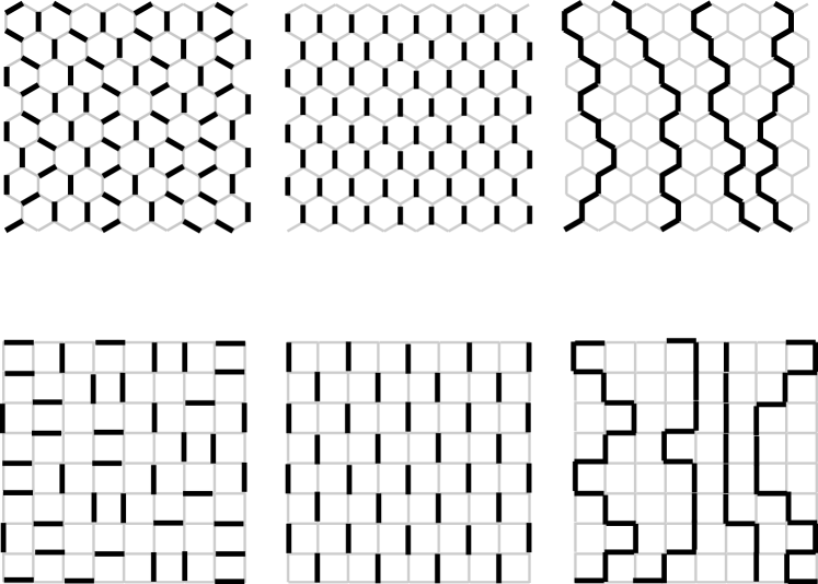
Figure 1: Mapping of dimer configurations to directed polymers by superposition with a fixed reference covering (middle).

III Clean system: continuum limit and thermodynamic ensembles

Before treating the random system, let us first compare the free energy density of the dimer models and the corresponding polymer lattice by taking the continuum limit. The free energy of dimer model on the hexagonal lattice can be computed exactly Yokoi-Nagle-Salinas-JSP . By changing variables from $z_{1}$, $z_{2}$ to $\eta=z_{1}/z_{2}$ and $\rho_{\hexagon}$, one can express the free energy density in terms of the physical quantities of the polymers on the lattice Jiang-Emig-preprint-2005 . The result is

$$f_{\rm dimer}=-\frac{2\pi}{\sqrt{3}}\int_{0}^{\rho_{\hexagon}}d\rho^{\prime}\frac{\eta\rho^{\prime}\sin(\pi\sqrt{3}b_{\hexagon}\rho^{\prime})}{1+\eta^{2}+2\eta\cos(\pi\sqrt{3}b_{\hexagon}\rho^{\prime})}\,,$$ (9)

where the energy is measured relative to the line $z_{1}+z_{2}=1$ of vanishing polymer density. For this expression we can take explicitly the continuum limit by sending $b_{\hexagon}\to 0$ while keeping the polymer density $\rho_{\hexagon}$ fixed, i.e., we adjust $z_{1}$ and $z_{2}$ so that the arcsin in Eq. (5) tends to zero $\sim b_{\hexagon}$ while $\eta=z_{1}/z_{2}$ is kept fixed. This yields the free energy density for the continuum version of the dimer model, expressed in terms of the polymer parameters,

$$f_{\rm dimer}=-\frac{\pi^{2}}{3}\frac{T}{g_{\hexagon}}\rho_{\hexagon}^{3}\,,$$ (10)

where we used Eq. (7).

An alternative approach to treat a system of interacting polymers in $(1+1)$ dimensions is to regard each polymer as a world line of a boson in imaginary time, leading to the quantum theory of interacting bosons in one spatial dimension. Choosing the imaginary time direction along the occupied bonds in the dimer reference state, the non-crossing constraint is naturally implemented by a hard core repulsion between the bosons which in one dimension is equivalent to non-interacting fermions. The Pauli principle then automatically prevents crossing. If the length $L_{y}$ of the polymers tends to infinity, their reduced free energy $L_{y}E_{0}/\hbar$ is given by ground state energy $E_{0}=(\pi^{2}/6)(\hbar^{2}/m)\rho^{3}L_{x}$ of 1D fermions at density $\rho$. Using the mapping $m\to g$ and $\hbar\to T$, one gets for the reduced free energy density of the polymers at fixed density

$$f_{\rm{poly}}=\frac{\pi^{2}}{6}\frac{T}{g}\rho^{3}\,.$$ (11)

Although the scaling of this result with the physical parameters is the same as for the free energy in the continuum limit of the dimer model, Eq. (10), the amplitudes do not agree. However, since in the dimer model the number of polymers is not fixed, we have to compare the dimer free energy with the potential of the grand canonical ensemble of the polymers. The chemical potential is obtained as $\mu=\partial f_{\rm poly}/\partial\rho=(\pi^{2}/2)(T/g)\rho^{2}$, yielding the grand canonical potential density

$$j_{\rm poly}=f_{\rm poly}-\mu\rho=-\frac{\pi^{2}}{3}\frac{T}{g}\rho^{3}\,,$$ (12)

which is in full agreement with the continuum limit of the exact solution of the dimer model of Eq. (10). This demonstrates that dimer model can be described on large length scales as free fermions where their mass is determined in terms of the bond weights by a random walk of a single polymer on the lattice.

It is instructive to compare the exact lattice result for the dimer free energy of Eq. (9) and the potential $j_{\rm poly}$ with $g_{\hexagon}$ of Eq. (7) even for larger $b_{\hexagon}\rho_{\hexagon}$. By numerical integration of Eq. (9), we obtain the ratio $f_{\rm dimer}/j_{\rm poly}$ over the entire range of possible polymer densities shown in Fig. 2. Up to approximately $1/4$ of the maximal density, we find reasonable agreement between the lattice and continuum results, almost independent of the anisotropy $\eta=z_{1}/z_{2}$. For larger densities the value of $\eta$ becomes important. There is an optimal value of $\eta$ close to $1/3$ for which the continuum description gives accurate results (within a few percent) even for all densities.

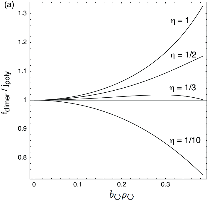
Figure 2: Comparison of the free energy $f_{\rm dimer}$ of the hexagonal lattice dimer model, Eq. (9), and the grand canonical potential $j_{\rm poly}$ of the continuum polymer system, Eq. (12) with the expression of Eq. (7) for $g/T$ substituted. The curves extend to $\rho_{\hexagon}=2/(3^{3/2}b_{\hexagon})$ which is the maximal polymer density on the lattice for $\eta=1$. However, in the lattice model, the density cannot become larger than $\rho_{\hexagon}=2/(\pi\sqrt{3})\arcsin(\sqrt{2+\eta}/2)$ by tuning the weights at a fixed ratio $\eta$.

The anisotropy of the dimer model can be tuned by changing the relative magnitude of the weights $z_{1}$ and $z_{2}$. The exact solution of the dimer model on the hexagonal lattice yields for the correlation lengths the result Yokoi-Nagle-Salinas-JSP

$$\xi_{x}=\frac{\sqrt{3}b_{\hexagon}}{2\phi_{0}}=\frac{1}{\pi\rho_{\hexagon}},\ \ \xi_{y}=\frac{3b_{\hexagon}}{4z_{1}z_{2}\phi_{0}\sin 2\phi_{0}}\,$$ (13)

with $\phi_{0}=\arcsin\sqrt{((z_{1}+z_{2})^{2}-1)/(4z_{1}z_{2})}$. Hence the correlation length perpendicular to the direction of the polymers is set by their mean distance $1/\rho_{\hexagon}$. The length $\xi_{y}$ should then be set by the typical scale a polymer can wander freely before it reaches a transverse displacement of the order of the mean distance between polymers. In the continuum description of the polymers, the random walk description of a single polymer then implies the relation

$$\xi_{x}^{2}=\frac{T}{g_{\hexagon}}\xi_{y}$$ (14)

between the correlation lengths. Together with the first relation of Eq. (13), this yields the anisotropy

$$\frac{\xi_{x}}{\xi_{y}}=\pi\frac{T}{g_{\hexagon}}\rho_{\hexagon}\,.$$ (15)

That this result is consistent with the anisotropy of the elastic description of the polymer system follows from the macroscopic compression modulus which is given by the compressibility, i.e., $c_{11}=T\rho^{2}\partial^{2}f_{\rm poly}/\partial\rho^{2}$ in terms of the reduced free energy of Eq. (11). This yields $c_{11}=\pi^{2}(T^{2}/g)\rho^{3}$ and hence together with $c_{44}=g\rho$

$$\frac{\xi_{x}}{\xi_{y}}=\sqrt{\frac{c_{11}}{c_{44}}}\,.$$ (16)

In order to connect the lattice and continuum description further, one would like to know under what conditions the lattice correlations lengths of Eq. (13) fulfill the continuum relation of Eq. (14). To address this question we change again variables from $z_{1}$, $z_{2}$ to $\eta=z_{1}/z_{2}$ and $\rho_{\hexagon}$. If one uses the result for $g_{\hexagon}$ of Eq. (7) one can easily check that Eq. (14) is indeed fulfilled in the continuum limit $b_{\hexagon}\to 0$. Hence, the exact anisotropy factor $\sqrt{c_{11}/c_{44}}$ of the continuum elastic model is recovered. This is important if one compares free energy densities of systems with different anisotropies since then the ratio of system sizes must be chosen as to match the ratio of their anisotropies.

For the dimer model on the square lattice, there is no direct analog of the previous analysis since the mean polymer density cannot be tuned by changing the weight $z_{1}$ but is fixed, see Eq. (6). Hence, one cannot take the continuum limit explicitly. Nevertheless, the square lattice is particular useful if one wants to study the effect of random bonds since the polymer density is robust against variations of the weights and thus shows no disorder induced fluctuations. For the clean square lattice dimer model, we can use the insight we gained from the previous analysis of the hexagonal lattice to compare the free energies of the square lattice and the continuum model. The exact reduced free energy density of the lattice model is known to be Kasteleyn-61-Fisher-61

$$f_{\rm dimer}=-\frac{1}{\pi b_{\Box}^{2}}\int_{0}^{z_{1}}dv\,\frac{\arctan v}{v}\,.$$ (17)

The continuum free fermion result of Eq. (12) yields in combination with the random walk result of Eq. (8) for the line tension on the square lattice the estimate for the reduced free energy density

$$f_{\rm dimer}=-\frac{\pi^{2}}{3}\frac{z_{1}b_{\Box}}{z_{1}+1/2}\,\rho_{\Box}^{3}\,.$$ (18)

Below we will study the square lattice with bond energies that are randomly distributed with mean zero so that the clean limit corresponds to the isotropic case $z_{1}=1$. For this case Eq. (17) yields the exact result $f_{\rm dimer}b_{\Box}^{2}=-G/\pi=-0.2916$ which is close to the continuum approximation of Eq. (18) which predicts $f_{\rm dimer}b_{\Box}^{2}=-\pi^{2}/36=-0.2742$ at the fixed density $\rho_{\Box}=1/(2b_{\Box})$.

IV Random bonds and pinned polymers

In this section we will consider exclusively the square lattice but with random energies $\epsilon_{ij}$ assigned to all vertical bonds so that $z_{ij}=\exp(-\epsilon_{ij}/T_{d})$, where $z_{ij}$ denotes now the weight on the bond $(ij)$. The dimer temperature $T_{d}$ measures the strength of disorder. The energies $\epsilon_{ij}$ are drawn for each bond independently from a Gaussian distribution with zero mean and unit variance. On all horizontal bonds we set $\epsilon_{ij}=0$ so that for $T_{d}\to\infty$ the isotropic clean dimer model is recovered. The partition function can be written as

$$Z_{\Box}=\sum_{\{D\}}\exp\left(-\sum_{(ij)\in D}\epsilon_{ij}/T_{d}\right)\,,$$ (19)

where the second sum runs over all occupied bonds. The disorder averaged free energy and correlations of this model have been computed by a polynomial algorithm Zeng-Leath-Hwa-PRL ; Elkies-Kuperberg-Larsen-Propp-JAC for system sizes up to $512\times 512$ lattice sites and typically $6000$ disorder samples Zeng-Leath-Hwa-PRL ; Bogner-Emig-Taha-Zeng-PRB .

On the analytical side, progress has been made for the polymer system with random pinning by applying the replica method. Regarding again each polymer of the replicated theory as a fermion in imaginary time, and applying the Pauli principle for all particles within the same replica, the replica free energy can be obtained again as the ground state energy of a one-dimensional system of fermions. Due to the replication, the fermions carry now $n$ spin components and interact via an attractive $\delta$-function potential arising from the short ranged disorder correlations. This $SU(n)$ fermi gas can be studied by a series of nested Bethe Ansätze Kardar-NPB . In the limit $n\to 0$, the Bethe Ansatz equations can be solved exactly for arbitrary disorder strength $\Delta$, yielding the disordered averaged reduced free energy density of the polymers Emig+03 ,

$$\bar{f}_{\rm poly}=\bar{f}_{0}(\Delta)\rho+\frac{\pi^{2}}{6}\frac{T}{g}\rho^{3}+\frac{\Delta}{2T^{2}}\rho^{2}\,,$$ (20)

where $\bar{f}_{0}(\Delta)$ represents the disorder dependent free energy of a single polymer. Notice the simple form of the disorder contribution to the free energy of the pure system, cf. Eq. (11). Interestingly, in the limit of strong interactions (disorder) the $SU(n)$ fermi gas in the limit $n\to 0$ becomes identical to the (pure) interacting Bose gas studied by Lieb and Liniger Lieb+Liniger . Since it was shown that the interaction strength scales as $n^{2}$, perturbation theory for the ground state energy of the Bose gas yields a series expansion in $n$ of the replica free energy for large disorder. The coefficients of this expansion correspond to the disorder averaged cumulants of the free energy which hence are known exactly from the replica Bethe Ansatz Emig-Kardar-NPB .

The prediction of the replica approach can be compared to the numerical evaluation of the free energy and its cumulant averages for the random bond dimer model. This has been done in Ref. Bogner-Emig-Taha-Zeng-PRB, , neglecting however fluctuations in the polymer density induced by the statistics of the pure dimer model. While nice agreement was found for the second and third cumulant of the free energy, the averaged free energies were only consistent if a term $\sim\Delta^{2}$ of the single polymer contribution $\bar{f}_{0}$ was dropped by hand. However, contributions $\sim n^{3}\Delta^{2}$ from the replica free energy of a single polymer were found to be crucial for the agreement of the third cumulant of the total free energy. A similar observation was made Bogner-Emig-Taha-Zeng-PRB for the data obtained previously for a single pinned polymer Krug+92 . This is in particular unsatisfying due to the model character of the directed polymer in a random potential for the theory of disordered systems. Below, we show that the differences between the replica approach for polymers and the numerical results on the dimer model can be fully reconciled when polymer density fluctuations are included. As demonstrated for the clean system, this can be done by comparing the canonical dimer ensemble to the grand canonical ensemble of polymers. From Eq. (20) follows the disorder averaged chemical potential $\bar{\mu}=\partial\bar{f}_{\rm poly}/\partial\rho$ since disorder induces no (additional) fluctuations in $\rho$. Thus, the average grand canonical potential density is

$$\bar{j}_{\rm poly}=-\frac{\pi^{2}}{3}\frac{T}{g}\rho^{3}-\frac{\Delta}{2T^{2}}\rho^{2}\,,$$ (21)

so that the single polymer term $\bar{f}_{0}$ cancels. Notice that $\bar{f}_{0}$ is exactly the term which was in disagreement with numerical results for the random bond dimer model. Hence, the disorder averaged free energy of a single directed polymer cannot be determined from numerical computations of the free energy of the dimer model. However, it is the disorder induced effective interaction of the polymers which determines the dimer free energy. To obtain the latter, we substitute the dimer parameters $\rho=\rho_{\Box}=1/(2b_{\Box})$ and $g/T$ from Eq. (8) into Eq. (21). The disorder strength $\Delta/T^{2}$ must be related to the dimer temperature $T_{d}$ which measures the variance of the bond energies. As was shown in Ref. Bogner-Emig-Taha-Zeng-PRB, the relation is

$$\frac{\Delta}{T^{2}}=\frac{\xi_{d}}{b_{\Box}}\frac{1}{T_{d}^{2}}\,,$$ (22)

where the length $\xi_{d}$ acts as a cutoff in the continuum model over which the $\delta$ function of Eq. (4) is smeared out. The ratio $\xi_{d}/b_{\Box}$ must be considered as a fitting parameter which should turn out to be of order unity. As we are comparing energy densities, the disorder dependent anisotropy $\sqrt{c_{11}/c_{44}}$ of the polymer system must be included Bogner-Emig-Taha-Zeng-PRB . This yields for the disorder averaged free energy density of the dimers

$$\bar{f}_{\rm dimer}=b_{\Box}^{2}\,\sqrt{\frac{c_{44}}{c_{11}}}\,\bar{j}_{\rm poly}\,.$$ (23)

The compression modulus can be obtained again from the (averaged) polymer free energy of Eq. (20), $c_{11}=T\rho^{2}\partial^{2}\bar{f}_{\rm poly}/\partial\rho^{2}$, yielding for the anisotropy

$$\sqrt{\frac{c_{44}}{c_{11}}}=\frac{1}{\pi\rho}\frac{g}{T}\left(1+\frac{g\Delta}{\pi^{2}T^{3}\rho}\right)^{-1/2}\,.$$ (24)

In order to correct for a (small) difference between lattice and continuum model, we match with the exact result $f_{\rm dimer}=-G/\pi$ of Eq. (17) with $z_{1}=1$ in the clean limit $T_{d}\to\infty$. Then we obtain in terms of the dimer parameters the final result

$$\bar{f}_{\rm dimer}=-\frac{G+\frac{3}{8}\frac{\xi_{d}}{b}T_{d}^{-2}}{\sqrt{\pi^{2}+3(\xi_{d}/b)T_{d}^{-2}}}\,,$$ (25)

which has to be compared to the result for $\overline{\ln Z_{l}}/L^{2}=-\bar{f}_{\rm dimer}$ of Eq. (32) in Ref. Bogner-Emig-Taha-Zeng-PRB, . The expression of Eq. (25) is plotted in Fig. 3 together with simulation data for the random dimer model, demonstrating indeed nice agreement for $\xi_{d}/b_{\Box}=1.33$.

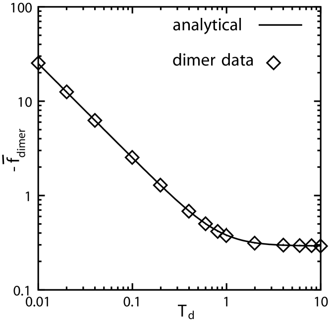
Figure 3: Disorder averaged free energy density for the random bond dimer model, Eq. (25) with $\xi_{d}/b_{\Box}=1.33$, and corresponding simulation data, taken from Ref. Bogner-Emig-Taha-Zeng-PRB, .

Finally, we comment on higher cumulant averages of the dimer free energy. They were also measured in simulations, and were shown to agree with the free energy fluctuations of the polymer system Bogner-Emig-Taha-Zeng-PRB . This can be easily understood from the fact that on the square lattice there are no sample-to-sample variations of the mean polymer density. Hence the shift of the polymer free energy by $-\mu\rho$ in Eq. (12) is independent of disorder so that one has identical disorder averaged cumulants in the canonical and grand canonical ensembles, $[j^{p}]_{c}=[f^{p}]_{c}$ for $p\geq 2$, where $[\ldots]_{c}$ denotes a cumulant average over disorder. Because of that, fluctuations of the single polymer free energy $f_{0}$ are important for the dimer model. This explains why contributions $\sim n^{3}\Delta^{2}$ from a single polymer to the replica free energy had to be included in Ref. Bogner-Emig-Taha-Zeng-PRB, to obtain agreement for the third cumulant of the free energy between polymer and dimer model.

V Outlook

We have shown that a continuum polymer model can provide a good approximation to dimer models on bipartite lattices. Although the polymer description yields in general not the exact result, it provides a more physical picture of the dimer model as its exact solution which, moreover, is available only in the clean limit. Lattice Ising spin models with geometric frustration can be mapped at zero temperature exactly to classical dimer models on the dual lattice Bloete . The effect of thermal fluctuations and/or a transverse magnetic field can be understood in terms of topological defects in the polymer representation of the dimer model Jiang-Emig-preprint-2005 . Here we have shown that the influence of random bonds in the dimer model can be described as pinning of polymers. This implies that the glassy state of certain spin models with random couplings could be related to the glass phase of polymers in a random environment. For example, it can be easily checked that random dilution of the triangular Ising antiferromagnet leads to a pinning of the polymers at the non-magnetic lattice sites. Another potential application of our results is the study of classical dimers which in addition to the hard-core repulsion interact in a more general way. Since the mapping to polymers is independent of the dimer interaction, one can use the analogy between directed polymers and world lines of bosons in imaginary time to explore dimer interactions in terms of interacting bosons in one dimension. Recently, the classical limit (without kinetic term) of the quantum dimer model on the square lattice has been shown to have a phase transition between a critical and a columnar phase due to the aligning interaction Alet+05 . The correlations in the critical phase are found to decay with an exponent that varies continuously with the interaction amplitude. Using the mapping to world lines of bosons, that exponent is determined by the compressibility of the bose gas which presumably can be modeled by a tight-binding Hamiltonian with an infinite on-site repulsion and a nearest neighbour interaction Affleck+04 .

- (1) D.S. Rokshar and S.A. Kivelson, Phys. Rev. Lett. 61, 2376 (1988)
- (2) R. Moessner and S.L. Sondhi, Phys. Rev. Lett. 86, 1881 (2001); G. Misguich, D. Serban and V. Pasquier, ibid. 89, 137202 (2002); R. Moessner and S.L. Sondhi, Phys. Rev. B 68, 184512 (2003)
- (3) R. Moessner and S.L. Sondhi, Phys. Rev. B 63, 224401 (2001)
- (4) Y. Jiang and T. Emig, Phys. Rev. Lett. 94, 110604 (2005)
- (5) S. Bogner, T. Emig, A. Taha, and C. Zeng, Phys. Rev. B 69, 104420 (2004)
- (6) C. Zeng, A. Middleton and Y. Shapir, Phys. Rev. Lett. 77, 3204 (1996)
- (7) P.W. Kasteleyn, Physica 27, 1209 (1961); M.E. Fisher, Phys. Rev. 124, 1664 (1961); M.E. Fisher and J. Stephenson, Phys. Rev. 132, 1411 (1963)
- (8) P.W. Kasteleyn, Jour. Math. Phys. 4, 287 (1963); M.E. Fisher, ibid. 7, 1776 (1966)
- (9) C.L. Henley, Jour. Stat. Phys. 89, 483 (1997)
- (10) H.W.J. Blöte and H.J. Hilhorst, Jour. Phys. A 15, L631 (1982); B. Nienhuis, H.J. Hilhorst and H.W.J. Blöte, ibib. 17, 3559 (1984)
- (11) Y. Jiang and T. Emig, Phys. Rev. B 73, 104452 (2005)
- (12) For a review, see T. Nattermann and S. Scheidl, Adv. Phys. 49, 607 (2000)
- (13) F. Alet, J. L. Jacobsen, G. Misguich, V. Pasquier, F. Mila, M. Troyer, Phys. Rev. Lett. 94, 235702 (2005).
- (14) M. Kardar, Nucl. Phys. B 290, 582 (1987)
- (15) T. Emig and M. Kardar, Nucl. Phys. B 604, 479 (2001)
- (16) C.S.O. Yokoi, J.F. Nagle, and S.R. Salinas, Jour. Stat. Phys. 44, 729 (1986)
- (17) C. Zeng, P.L. Leath, and T. Hwa, Phys. Rev. Lett. 83, 4860 (1999)
- (18) N. Elkies, G. Kuperberg, M. Larsen, and J. Propp, Jour. Algebr. Comb. 1, 111 (1992); 219 (1992)
- (19) T. Emig and S. Bogner, Phys. Rev. Lett. 90, 185701 (2003).
- (20) E.H. Lieb, W. Liniger, Phys. Rev. 130, 1605 (1963).
- (21) J. Krug, P. Meakin, and T. Halpin-Healy, Phys. Rev. A 45, 638 (1992).
- (22) I. Affleck, W. Hofstetter, D. R. Nelson, and U. Schollwöck, J. Stat. Mech.: Theor. Exp. P10003 (2004).