Many-body studies
on atomic quantum systems

          Many-body studies
          on atomic quantum systems

Memòria presentada per	Programa de doctorat
Jordi Mur Petit	Física Avançada
per optar al títol de	del Departament d’Estructura
Doctor en Ciències Físiques.	i Constituents de la Matèria,
Barcelona, novembre 2005.	bienni 2000-2002,
	Universitat de Barcelona.

Director de la tesi:	Prof. Artur Polls Martí
	Catedràtic de Física Atòmica, Molecular i Nuclear
	Universitat de Barcelona

Tribunal:	Dr. Martí Pi, president del tribunal
	Dra. Muntsa Guilleumas, secretària del tribunal
	Prof. Maciej Lewenstein
	Prof. Giancarlo C. Strinati
	Dr. Jordi Boronat

a

A la meva família
i en especial a la meva mare

a

Contents

1. Agra ments
2. Plan of the thesis
3. I Ultracold gases
   1. 1 The pairing solution
      1. 1.1 Historical background: before bcs theory
      2. 1.2 The Bardeen-Cooper-Schrieffer theory
         1. 1.2.1 Premier: Cooper pairs
         2. 1.2.2 Formalism for the theory
         3. 1.2.3 An easy example: the symmetric case
      3. 1.3 Summary
   2. 2 Pairing in density-asymmetric fermionic systems
      1. 2.1 Introduction
      2. 2.2 Pairing in $s$-wave
      3. 2.3 Numerical results
         1. 2.3.1 The algorithm
         2. 2.3.2 Symmetric case
         3. 2.3.3 Asymmetric case
      4. 2.4 Pairing in $p$-wave
      5. 2.5 Summary
   3. 3 Pairing with broken space symmetries: loff vs. dfs
      1. 3.1 Introduction
      2. 3.2 Breaking the symmetry: loff and dfs
         1. 3.2.1 Description of the loff state
         2. 3.2.2 Description of the dfs state
      3. 3.3 The gap in the bcs, loff and dfs phases
      4. 3.4 Excitation spectra in the superfluid phases
      5. 3.5 Determining the ground state
         1. 3.5.1 Calculation of the free energy
         2. 3.5.2 Analytical estimation of the optimal deformation
         3. 3.5.3 Numerical results
      6. 3.6 Detecting the dfs phase in experiments
      7. 3.7 Summary
   4. 4 Pairing in boson-fermion mixtures
      1. 4.1 Introduction
      2. 4.2 Three-dimensional mixtures
      3. 4.3 Two-dimensional mixtures
         1. 4.3.1 Constant T-matrices
         2. 4.3.2 Energy-dependent T-matrices
         3. 4.3.3 Prospects of experimental detection
      4. 4.4 Discussion
   5. 5 Dynamics of spin-1 condensates at finite temperatures
      1. 5.1 Introduction
      2. 5.2 Formalism
         1. 5.2.1 Ground state of the homogeneous system
         2. 5.2.2 Dynamical equations and transfer of population
      3. 5.3 Numerical procedure
      4. 5.4 Dynamical evolution at zero temperature
      5. 5.5 Dynamical evolution at finite temperature
         1. 5.5.1 Introducing temperature fluctuations
         2. 5.5.2 Results for a ‘ferromagnetic’ system: ⁸⁷Rb
         3. 5.5.3 An ‘antiferromagnetic’ system: ${}^{87}\mbox{Rb}_{\mathrm{AF}}$
      6. 5.6 Conclusions
4. II Two-dimensional helium systems
   1. Motivation: helium as ‘the’ quantum liquid
   2. 6 Quantum Monte Carlo study of ⁴He clusters
      1. 6.1 Short introduction to Quantum Monte Carlo methods
         1. 6.1.1 Importance sampling and Metropolis algorithm
         2. 6.1.2 Variational Monte Carlo
         3. 6.1.3 Diffusion Monte Carlo
         4. 6.1.4 Building the trial function
      2. 6.2 vmc ground-state energies
      3. 6.3 dmc ground-state energies
      4. 6.4 Energy and line tension: introducing the mass formula
      5. 6.5 vmc and dmc density profiles
         1. 6.5.1 Calculating pure estimators
         2. 6.5.2 Numerical results
      6. 6.6 Summary and conclusions
   3. 7 Density Functional study of ⁴He non-homogeneous systems
      1. 7.1 Introduction to Density Functional theory
         1. 7.1.1 The Hohenberg-Kohn theorem
      2. 7.2 Semi-infinite system and slabs
      3. 7.3 Drops and line tension
      4. 7.4 Hydrodynamic equilibrium in a droplet
      5. 7.5 Discussion of the results
         1. 7.5.1 2D and 3D slabs in Density Functional theory
         2. 7.5.2 2D clusters according to df and qmc calculations
      6. 7.6 Summary and conclusions
   4. A Summing up over fermionic Matsubara frequencies
   5. B Deduction of the equations of motion of spin-$f$ condensates
      1. B.1 Introduction
      2. B.2 Mean-field dynamical equations for a spin-1 condensate
      3. B.3 Mean-field dynamical equations for a spin-2 condensate

List of Figures

1. 1.1 The Cooper problem
2. 1.2 Momentum distribution and excitation energies in bcs
3. 1.3 Diagrammatic representation of the T-matrix
4. 2.1 Evaporative cooling procedure
5. 2.2 The two possible lowest-order pairing interactions
6. 2.3 bcs momentum distributions in asymmetric matter
7. 2.4 Numerical solution for the symmetric case varying $k_{F}|a|$
8. 2.5 Numerical solution for the symmetric case varying $T$
9. 2.6 Numerical solution for the asymmetric case varying $\alpha$
10. 2.7 Variation of the gap with density asymmetry
11. 2.8 Third order diagrams in a one-component system
12. 3.1 Dependence of loff and dfs gaps on asymmetry
13. 3.2 bcs and dfs quasiparticle spectra
14. 3.3 bcs, loff and dfs critical asymmetries
15. 3.4 loff and dfs free energies vs. density asymmetry
16. 3.5 Occupation probabilites of the two hyperfine states
17. 4.1 Boson-induced interactions in two and three dimensions
18. 4.2 Diagrammatic contributions to the induced interaction
19. 4.3 Possible collision events in a Bose-Fermi mixture
20. 4.4 The optimal values $x_{\rm opt}$ and $h_{\rm opt}$ for the induced interaction
21. 4.5 The pairing gap for optimal boson concentration
22. 5.1 The Euler angles $\{\alpha,\beta,\gamma\}$ that define a rotation
23. 5.2 Population of the spin components vs. time at $T=0$
24. 5.3 Density profiles of the spin components vs. time at $T=0$
25. 5.4 Effective potentials and population transfers vs. time at $T=0$
26. 5.5 Population of the spin components vs. time at $T=0.2T_{c}$
27. 5.6 Density profiles of the spin components vs. time at $T=0.2T_{c}$
28. 5.7 Populations vs. time for an ‘antiferromagnetic’ system
29. 5.8 Density profiles for an ‘antiferromagnetic’ system at $T$=$0.2T_{c}$
30. 6.1 Flow chart of the Metropolis algorithm
31. 6.2 Aziz HFD-B(HE) interaction potential for ⁴He atoms
32. 6.3 Energies per particle of $N$-atom puddles vs. $N^{-1/2}$
33. 6.4 Why do we loose binding energy in a finite system?
34. 6.5 Convergence of the future walking method
35. 6.6 Density profiles of ⁴He puddles with various numbers of atoms
36. 7.1 Sketches of the semi-infinite medium and a slab
37. 7.2 Energy per particle and chemical potential of slabs
38. 7.3 Density profiles of slabs with varying central densities
39. 7.4 Radius and thickness of slabs as a function of coverage
40. 7.5 Energy per particle and chemical potential of droplets
41. 7.6 Density profiles of droplets with varying number of atoms
42. 7.7 Central density and rms radius of various droplets
43. 7.8 Pressure profile in the clusters with $N=36,10^{4}$ atoms
44. 7.9 Forces on an area of a two-dimensional drop
45. 7.10 Comparison of the 2D and 3D equations of state
46. 7.11 Comparison among vmc, dmc and df density profiles
47. A.1 Complex $z$-plane with the contours $C$ and $C^{\prime}+\Gamma$.

List of Tables

1. 3.1 The various candidates for a superfluid ground state studied.
2. 6.1 vmc ground-state energy per particle of various ⁴He clusters
3. 6.2 dmc ground-state energy per particle of various ⁴He clusters
4. 6.3 Coefficients of a fit of the mass formula and line tension
5. 6.4 Parameters of a Fermi-profile fit to the dmc density profiles
6. 7.1 Parameters of the two-dimensional zero-range functional
7. 7.2 Parameters of a Fermi-profile fit to the df density profiles

Agra ments

Buf! Vet-ho aqu el primer que em ve al cap en pensar que ja he acabat d’escriure el que hauria de ser el resum de la meva tasca els darrers cinc anys i escaig. Unes cent seixanta p gines de ci ncia <<pura i dura>>. Quina pallisa, no? Per aquest resum estaria excessivament esbiaixat cap a la feina feta si no dediqu s ni que fossin quatre ratlles per mirar enrere tamb en el pla personal. Ben mirat, dif cilment hauria pogut fer res del que cont aquesta tesi sense la interacci amb una petita multitud de gent amb qui sens dubte he evolucionat tamb com a persona. Probablement m s que no pas com a cient fic; al capdavall, tot just ara puc comen ar a anomenar-me aix .

En primer lloc, haig d’agrair a l’Artur haver-me acollit com a doctorand i haver-se <<atrevit>> a iniciar amb mi la recerca en un camp nou, el dels toms freds, que l’any 2000 —que lluny sona, sembla que parli del segle passat!— estava en plena explosi … i encara no ha parat. Els mal-de-caps que hem tingut perseguint la literatura per posar-nos al dia! La teva voluntat pel di leg de ben segur ha estat ingredient imprescindible per l’ xit d’aquesta empresa. Vull agrair tamb a la Muntsa, la nostra experta local en BEC, estar sempre disposada a escoltar-me i xerrar una estona, ja sigui de f sica o del que convingui.

No puc oblidar-me tampoc dels altres membres del grup, passats i presents, que han fet de les moltes hores passades al departament una experi ncia d’all m s enriquidora. L’ ngels, que em va acollir iniciament amb l’Artur, si b despr s els nostres camins cient fics s’han separat lleugerament. L’Isaac i, especialment, la Laura amb qui vaig compartir no nom s l’assoleiat despatx 652 sin tamb moltes bones estones. I l’Assum, baixllobregatina com un servidor i amb qui vaig connectar r pidament (potser per all de compartir el tel fon durant tant de temps?). Dels primers temps a ECM tamb haig de recordar el Hans, il tedesco piu’ specialle che ho mai trovato, amante della montagna, di Catania e della <<Cerveceria Catalana>>, con cui ho imparato una sacco su pairing.

M s recentment, ha estat especialment engrescadora i estimulant la relaci amb els <<encontradors>>, l’Arnau i l’Oliver, amb qui hem demostrat que disposar d’un pressupost zero no s obstacle per organitzar un exit s cicle de xerrades. Les reunions d’organitzaci , sovint sessions de deliri mental conjunt, ens han dut a reinterpretar Einstein i fins i tot sortir a la p gina web de la UB i a <<el Pa s>>. Qu m s podem demanar? Amb l’Arnau tamb vam tenir el plaer d’estrenar el nou despatx <<cara al sol>>, juntament amb el Chumi, que amb els seus apunts tutti colori i cartells teatrals hi ha aportat un toc ben especial.

Per acabar amb l’entorn <<laboral>>, vull mencionar il professore Brualla, de capacitat verbal inacabable, sigui en catal , angl s o itali i que sempre t una an cdota a la butxaca per il$\cdot$lustrar una conversa. El Jes s, <<catal del sud>> que em va acollir durant un parell de visites a Val ncia i pel qual vaig anar a Finl ndia —afortunadament, a l’agost— per aprendre density functional. I, com no, la Mariona, que no es va espantar en fer la beca de col$\cdot$laboraci i s’ha incorporat definitivament al grup. Et desitjo molta sort en aquesta aventura que ara emprens. Per comen ar, la cosa pinta b : t’acaben d’atorgar una beca de la famosa(?) Fundaci Agust Pedro i Pons. La mateixa beca a mi em va permetre de sobreviure durant el primer any de doctorat, cosa que vull agrair tamb aqu .

Dit aix potser hauria d’agrair tamb la Gene, no? Deixant de banda les lli ons de <<burocr cia creativa>> que les renovacions anuals comporten, vull agrair sobretot les borses de viatge, que m’han perm s agafar el <<gustet>> a aix de viatjar. He pogut anar per mitja Europa i un bon tros dels E.U.A., i he fet una colla d’amics. Primer vaig anar a Pisa, a treballar amb Adelchi Fabrocini: grazie per accogliermi e per aiutarmi a imparare un po’ la lingua di Dante. Anche altri membri del gruppo (sopratutto Ignazio), del dipartimento (Marco e i suoi collegi sperimentali, insieme a Eleonora) e dell’Universit (ricordo specialmente i miei coinquillini a via San Frediano: Manu, Gigi, Max e anche Maria Luisa) hanno fatto un buon lavoro in questo senso.

Posteriorment vaig anar a treballar amb el grup d’Anna Sanpera i Maciej Lewenstein a Hannover. Els agraeixo, juntament amb els altres membres del grup (Ver nica, Kai, Florian, Helge, Alem) la seva amistat i les estimulants xerrades mantingudes.

Finalment, fa pocs mesos he pogut <<fer les Am riques>> visitant el grup de Murray Holland al JILA de Boulder. My stay turned out to be too short to finish a project, but long enough to enjoy the hospitality and friendship of you and the people in your group (Meret, Stefano, Rajiv, Brian, Jochen, Lincoln and Maril ). I also want to thank Svet, Michele and Cindy for friendship and illustrative discussions. Y, como no, la pe a de ‘exiliados hispanohablantes’ (Manolo de Madrid, Fernando, Mar a, Elena y B rbara, Vitelia, Manolo de Sevilla) que hicieron m s llevadera la distancia espacial y temporal con mi ‘casita’.

Parlant d’amics, vull mencionar tamb l’H ctor, amic literalment <<de tota la vida>> i amb qui el b squet m’ha unit de nou per viure grans moments al Palau. I l’Ivan, amic amb qui em trobo menys del que voldria, gr cies al qual vaig contactar amb l’Esther que, en una recerca digna de Sherlock Holmes, va ser capa de trobar una agulla en un paller, o el que s el mateix, una cita dins tota l’obra de Shakespeare.

I aix em porta a recordar els de casa, indispensables en la meva vida i sense els quals no seria res. Durant aquests darrers anys hem passat per moltes coses; hi ha qui ha marxat, i qui ha arribat, i mai m’ha faltat el vostre suport. Sobretot vull destacar la meva mare, Teresa, que s qui m’ha hagut de suportar m s hores —i aix de vegades s ben dif cil!—: perqu la teva capacitat d’esfor i superaci en l’adversitat s n un model a seguir. El meu pare, Miquel, que no es va voler rendir mai en la dificultat: cada cop que viatjo enyoro m s els teus consells —que abans no sempre vaig saber apreciar. Els meus germans, Rosa i Ferran, aix com el Pep i la Viole: no puc oblidar els vostres nims en els meus primers viatges a fora, quan no estava segur de com aniria tot plegat i rebre una trucada o un mail era sempre una alegria. I els <<reis de la casa>>, l’Enric i la N ria, font inesgotable d’an cdotes per compartir i recordar, i amb qui s ben f cil d’aprendre una cosa nova cada dia.

Sant Boi de Llobregat, 22 de novembre de 2005

Plan of the thesis

During the last five years, I have been learning some of the theoretical tools of Many-Body physics, and I have tried to apply them to the fascinating world of quantum systems. Thus, the studies presented in this thesis constitute an attempt to show the usefulness of these techniques for the understanding of a variety of systems ranging from ultracold gases (both fermionic and bosonic) to the more familiar helium. The range of techniques that we have used is comparable to the number of systems under study: from the simple, but always illustrative mean-field approach, to the powerful Green’s functions’ formalism, and from Monte Carlo methods to the Density Functional theory.

I have made an effort to present the various works in an understandable way. I would like to thank Prof. Artur Polls, my advisor, and Dr. Lloren Brualla, Dr. Muntsa Guilleumas, Prof. Jes s Navarro and Dr. Armen Sedrakian for carefully reading various parts of the manuscript, raising interesting questions and suggesting improvements. In any case, of course, any error or misunderstanding should be attributed only to me. I’ll be glad to receive questions or comments on any point related to this work.

The plan of the thesis is as follows. In a first part, we study ultracold gases of alkali atoms. The first three chapters are devoted to the evaluation of the possibilities of having and detecting a superfluid system of fermionic atoms. The first chapter introduces the idea of pairing in a Green’s functions’ formulation of the theory of superconductivity by Bardeen, Cooper and Schrieffer. Chapter 2 presents the application of this theory to the case of a two-component system where the two species may have different densities, a fact that has important consequences for the prospects of superfluidity. This work was performed in collaboration with Dr. Hans-Josef Schulze who, at that time, was a post-doc in Barcelona. Many of the results expounded here have appeared in the article [MPS01].

Chapter 3 generalizes the structure of the bcs ground state to the cases of finite-momentum Cooper pairs (the so-called loff or fflo phase) and deformed Fermi surfaces (dfs). This last state was first proposed by Prof. Herbert M ther and Dr. Armen Sedrakian from Universit t T bingen, with whom we have worked together and who I would like to thank for their warm hospitality during my visits to T bingen. As a result of this work, we have recently published the paper [SMPM05].

Chapter 4 introduces for the first time bosons into this thesis. They are used to cool a one-component system of fermions, and their capacity to help the fermions to pair is studied, with emphasis in the case of a two-dimensional configuration. This research, which appeared in [MPBS04b] and in [MPBS04a], was performed again with Dr. Schulze, then in Catania, and with Prof. Marcello Baldo. I want to thank both of them, and the rest of the infn group for their friendship and hospitality during my visit in 2003.

In chapter 5 we enter boldly into the world of bosonic systems and analyze the dynamical evolution of a set of bosons whose spin degree of freedom is free to evolve inside an optical trap, only restricted by the conservation of magnetization. An attempt to incorporate temperature effects is also performed. Thanks to this project I could enjoy for a couple of months the stimulating atmosphere in the group of Prof. Maciej Lewenstein and Prof. Anna Sanpera at Universit t Hannover, just before they moved to Catalonia. This work, developed in close collaboration with the experimental group of Prof. K. Sengstock and Dr. K. Bongs from Universit t Hamburg, has been submitted for publication to Physical Review A [MGS⁺05].

At the conceptual half of the thesis (p. II), we leave ultracold gases and start the study of helium-4 in two dimensions, which constitutes the second part of the work. First, in chapter 6, we present a Monte Carlo study of the ground-state structure and energetics of ⁴He puddles, with an estimation of the line tension. The results obtained here are incorporated in chapter 7 to build a Density Functional appropiate to study two-dimensional helium systems. This functional is then used to analyze a variety of such systems, and a comparison with previous studies in two and three dimensions is presented. Both these works have been developed in collaboration with Prof. Jes s Navarro, from CSIC-Universitat de Val ncia, and Dr. Antonio Sarsa, who is now at Universidad de C rdoba. Some of the results presented here have appeared in [SMPN03] and [MSNP05].

The conclusions of the thesis are finally summarized.

Part I Ultracold gases

Chapter 1 The pairing solution

—Bien parece —respondi don Quijote— que no est s cursado en esto de las aventuras: ellos son gigantes; y si tienes miedo, qu tate de ah , y ponte en oraci n en el espacio que yo voy a entrar con ellos en fiera y desigual batalla. (…) ¡Non fuyades, cobardes y viles criaturas, que un solo caballero es el que os acomete!

Miguel de Cervantes, Don Quijote de la Mancha (I, 8)

1.1 Historical background: before bcs theory

The bcs  theory of superconductivity [BCS57, Sch88] has been one of the most successful contributions to physics in the 20^th century, because it was the first microscopic theory of a truly macroscopic quantum phenomenon. It explains the mechanisms behind dissipation-free electric transport in a number of materials. Indeed, since its formulation, this theory has been applied to such different systems as solid metals and alloys [Sch88, dG66], atomic nuclei and neutron stars [BMP58, DH03], elementary particle physics (see, e. g., [CN04]) and superfluid ³He [ORL72, Leg75].

The theory developed by Bardeen, Cooper and Schrieffer appeared as a final step in the theoretical understanding of a long series of experimental discoveries. In 1911 Heike Kamerling Onnes [Kam11] observed that mercury below 4.2 K looses its electrical resistance and enters ‘a new state, which, owing to its particular electrical properties, can be called the state of superconductivity’ [Kam67]. In 1933 Meissner and Ochsenfeld [MO33] observed that a superconductor has also notable magnetic properties, namely it is a perfect diamagnet: a (small) applied magnetic field vanishes in the interior of a bulk superconductor. Another important contribution was the discovery in 1950 of the isotope effect (i. e., the dependence of the critical temperature on the mass of the ions of a superconducting solid) by Maxwell [Max50] and Reynolds et al. [RSWN50]. Finally, let us mention the experimental determination of the quantization of the magnetic flux traversing a multiply-connected superconductor by Deaver and Fairbank [DF61] and Doll and N bauer [DN61] following an initial prediction of the London model.

There were many theoretical attemps to explain the experimental results prior to the theory of Bardeen, Cooper and Schrieffer. In a first phenomenological theory, Gorter and Casimir [GC34] formulated a two-fluid model (similar to that of Tisza [Tis38, Tis40] and Landau [Lan41] for ⁴He) where electrons can be either in a superconducting state or in the normal state. At $T=0$ all electrons are in the superfluid, while the fraction of normal electrons grows with temperature and finally equals one at the critical temperatre $T_{c}$. The fraction of normal electrons was calculated by minimazing a free energy interpolated between the limits of a superfluid system at $T=0$ and a normal one at $T=T_{c}$. This model, however, had a number of artificial points (such as the way to construct the free energy), just intended to reproduce the experimental results known at the moment, but without a microscopic physical motivation.

A more successful theory was that of F. London and H. London [LL35, Lon35] based on the electromagnetic phenomenology of supercondutors. It explained the Meissner-Ochsenfeld effect [MO33], introduced a ‘penetration length’ $\lambda$ of magnetic fields into superconductors and also predicted the quantization of magnetic flux in a multiply-connected superfluid. F. London’s work also speculated on the possible existence of a gap in the excitation spectrum of a superfluid, a crucial ingredient in bcs theory.

In 1950 Ginzburg and Landau [LG50] formulated a non-local theory of superconductivity by generalizing the ideas of the London brothers: they introduced a spatially-varying ‘order parameter’ closely related to Londons’ superfluid density. This theory was valid only near $T_{c}$, but nevertheless it became of great interest with the discovery of type II superconductors. It is worth noticing that Ginzburg and Landau’s theory can be also derived from the bcs microscopic theory [Gor59].

In 1956, Cooper [Coo56] studied the problem of an interacting pair of fermions above a frozen Fermi sea and showed that, for an attractive interaction (no matter how weak it was), the pair would be bound, with an exponentially small binding energy in the limit of small coupling. These bound pairs are called ‘Cooper pairs’, and are a central ingredient of the bcs theory of superconductivity: Assuming that all the electrons in a metal are forming such pairs one can show that the total energy of the system is lowered with respect to that of the normal system.

1.2 The Bardeen-Cooper-Schrieffer theory

In this section, we introduce the microscopic theory of superconductivity of Bardeen, Cooper and Schrieffer (know as ‘bcs theory’) in a way that will later allow us to apply it to a variety of atomic gases as we shall do in the following chapters. We will start in Sect. 1.2.1 by introducing the idea of Cooper pairs and show how the presence of a Fermi sea allows an interacting pair of fermions to bind itself at arbitrary small attraction. This many-body effect (in the sense that the pair would not be bound in the absence of the Fermi sea unless the attraction was greater than a minimum value) is the essence of bcs theory, which we present in a formal way in Sect. 1.2.2. Finally, we present some basic results of the theory in Sect. 1.2.3.

1.2.1 Premier: Cooper pairs

Consider a pair of fermions of mass $m$ in homogeneous space above a ‘frozen’ Fermi sea of non-interacting particles with Fermi energy $\varepsilon_{F}=\hbar^{2}k_{F}^{2}/2m$. Let us assume that these two particles are distinguishable (for example, they can be electrons with different spins, atoms of the same chemical element with different hyperfine spins, neutrons and protons, or quarks of different colors), and that they interact through a two-body spin-independent potential. The presence of the Fermi sea forbids the particles from occupying the energy levels below $\varepsilon_{F}$ (see Fig. 1.1). Therefore, we can take $\varepsilon_{F}$ as their zero-energy level. This problem was originally solved by Cooper [Coo56], so it is usually called the ‘Cooper problem’ and the bound pairs are known as ‘Cooper pairs’. The solution we describe is based on [Sch88].

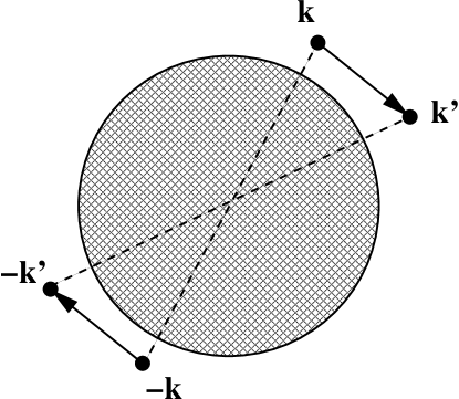
Figure 1.1: The Cooper problem: two fermions in states $|\bm{k}\rangle$ and $|-\bm{k}\rangle$ interact above a frozen Fermi sea (filled sphere). The fermions form a pair (dashed line) with center-of-mass momentum $\bm{q}=\bm{0}$ and can scatter into states $|\bm{k^{\prime}}\rangle$ and $|-\bm{k^{\prime}}\rangle$ for $|\bm{k^{\prime}}|>k_{F}$.

The wave function of a pair with momentum $\bm{q}$ in the center-of-mass system (c.m.s.) can be written

$$\psi(\bm{x}_{1},\bm{x}_{2})=\phi_{\bm{q}}(\bm{r})\exp\{i\bm{q}\cdot\bm{R}\}\;,$$

where we have defined the centre-of-mass coordinate $\bm{R}=(\bm{x}_{1}+\bm{x}_{2})/2$ and the relative coordinate $\bm{r}=\bm{x}_{1}-\bm{x}_{2}$. Taking for simplicity $\bm{q}=\bm{0}$, we have

$$\psi=\phi(\bm{r})=\sum_{k>k_{F}}a_{\bm{k}}e^{i\bm{k}\cdot\bm{r}}=\sum_{k>k_{F}}a_{\bm{k}}e^{i\bm{k}\cdot\bm{x}_{1}}e^{-i\bm{k}\cdot\bm{x}_{2}}\;.$$ (1.1)

Here we have applied Pauli’s exclusion principle to restrict the summations over momenta to the region outside the filled Fermi sea. This wave function can be interpreted as a superposition of configurations with single-particle wave functions with momenta $|\bm{k}\rangle$ and $|-\bm{k}\rangle$.

The corresponding Schr dinger equation can be written

$$(E-H_{0})\psi =V\psi\quad\Rightarrow\quad(E-2\epsilon_{\bm{k}})a_{\bm{k}}=\sum_{k^{\prime}>k_{F}}V_{\bm{k}\bm{k^{\prime}}}a_{\bm{k^{\prime}}}\;,$$ (1.2)

$$V_{\bm{k}\bm{k^{\prime}}} :=\left\langle\bm{k},-\bm{k}|V|\bm{k}^{\prime},-\bm{k}^{\prime}\right\rangle\;,$$

where we have introduced the single-particle spectrum $\epsilon_{\bm{k}}$ corresponding to $H_{0}=-\hbar^{2}\nabla^{2}/(2m)$.

If we take the simple case of a constant, attractive interaction constrained to a shell of width $\Omega$ above the Fermi surface, that is,

$$V_{\bm{k}\bm{k^{\prime}}}=\left\{\begin{array}[]{cl}-|\lambda|&\varepsilon_{F}<\epsilon_{\bm{k}},\epsilon_{\bm{k^{\prime}}}<\varepsilon_{F}+\Omega\\ 0&\mathrm{otherwise}\end{array}\right.\;,$$

then the lowest eigenenergy is

$$E=2\varepsilon_{F}-\frac{2\Omega}{\exp\left[\frac{2}{\nu(k_{F})|\lambda|}\right]-1}\simeq 2\varepsilon_{F}-2\Omega e^{-\frac{2}{\nu(k_{F})|\lambda|}}\;,$$ (1.3)

where $\nu(k_{F})=mk_{F}/(2\pi^{2}\hbar^{2})$ is the density of single-particle states for a single spin projection at the Fermi surface. The last result is valid in the weak-coupling approximation, $\nu(k_{F})|\lambda|\ll 1$.

Therefore, the pair will be bound ($E<2\varepsilon_{F}$) no matter how small $|\lambda|$ is. Note that this is a truly many-body effect as, in the absence of the underlying, filled Fermi sea, the pair would not bind for too weak an interaction. Furthermore, the non-analytic behavior in the weak-coupling limit shows that this result could not be found by perturbation theory, as it corresponds to a deep modification of the ground state as compared to the ideal Fermi gas.

1.2.2 Formalism for the theory

Let us study now a more realistic problem in which we have an interacting system of fermions with an internal degree of freedom, that we indicate by a (pseudo)spin variable $s=\uparrow,\downarrow$. This problem can be modeled by the following second-quantized Hamiltonian

$$\hat{H}=\sum_{s}\int\mathrm{d}^{3}x\,\hat{\psi}^{\dagger}_{s}(\bm{x})\left(-\frac{\hbar^{2}}{2m}\nabla^{2}\right)\hat{\psi}_{s}(\bm{x})\\ +\frac{1}{2}\int\mathrm{d}^{3}x\,\int\mathrm{d}^{3}x\,\!^{\prime}\,V(\bm{x}-\bm{x^{\prime}})\hat{\psi}^{\dagger}_{\downarrow}(\bm{x})\hat{\psi}^{\dagger}_{\uparrow}(\bm{x^{\prime}})\hat{\psi}_{\uparrow}(\bm{x^{\prime}})\hat{\psi}_{\downarrow}(\bm{x})$$ (1.4)

Here, $\hat{\psi}_{s}(\bm{x})\leavevmode\nobreak\ (\hat{\psi}^{\dagger}_{s}(\bm{x}))$ is the operator that destroys (creates) a particle of (pseudo)spin $s$ at position $\bm{x}$, and $V(\bm{x}-\bm{x^{\prime}})$ is the interaction potential between the fermions. We will be interested in low-density, low-temperature systems where the most important contribution to interactions is the $s$-wave one.

We look for a solution to this problem using the tools of quantum field theory, in particular, the Green’s functions’ formalism. We start linearizing the interaction and transforming it into a one-body operator by means of a Hartree-Fock-like approximation,

$$\hat{V}_{\rm HF}=\sum_{s}\int\mathrm{d}^{3}x\,\!\!\int\mathrm{d}^{3}x\,\!^{\prime}\;V(\bm{x}-\bm{x^{\prime}})\Big{\{}\left\langle\hat{\psi}^{\dagger}_{s}(\bm{x})\hat{\psi}_{s}(\bm{x})\right\rangle\hat{\psi}^{\dagger}_{-s}(\bm{x^{\prime}})\hat{\psi}_{-s}(\bm{x^{\prime}})\\ +\left\langle\hat{\psi}^{\dagger}_{s}(\bm{x})\hat{\psi}_{-s}(\bm{x^{\prime}})\right\rangle\hat{\psi}^{\dagger}_{-s}(\bm{x^{\prime}})\hat{\psi}_{s}(\bm{x})\Big{\}}\>.$$ (1.5)

The first term inside the curly brackets is the direct (or Hartree) term, while the second one is the exchange (or Fock) one. In the next step, we consider a new term in the linearization process which accounts for the possibility, outlined in the previous section, that two fermions with opposite spins form a bound pair (cf. Sec. 51 in [FW71] or Sec. 7-2 in [Sch88]). Even though $\hat{H}$ commutes with the number operator $\hat{N}$, this pairing possibility is more easily implemented if we work in the grand-canonical ensemble. Physically, we can understand this in the following way: for a large number of particles $N$ in the system, the ground state energies of the system with $N$ and $N\pm 1$ particles are nearly degenerate if we substract from them the chemical potential. Then, it is reasonable that a wave function in Fock space, with only the average value $N=\langle\hat{N}\rangle$ fixed, is more flexible from a variational point of view than one with a fixed number of particles. In this way, the function can be closer to the true ground state of the system immersed in the ‘bath’ of condensed pairs. In fact, it is customary to assume that the Hartree-Fock potential above is the same in the normal and superfluid states, so that we can disregard it from now on as its inclusion would not affect the comparison between both states. Therefore, we will work with the following effective (grand-canonical) Hamiltonian

$$\hat{K}=\sum_{s}\int\mathrm{d}^{3}x\,\hat{\psi}^{\dagger}_{s}(\bm{x})\left(-\frac{\hbar^{2}}{2m}\nabla^{2}-\mu_{s}\right)\hat{\psi}_{s}(\bm{x})+\int\!\mathrm{d}^{3}x\int\!\mathrm{d}^{3}x^{\prime}\,V(\bm{x}-\bm{x^{\prime}})\times\\ \times\left[\left\langle\hat{\psi}^{\dagger}_{\downarrow}(\bm{x})\hat{\psi}^{\dagger}_{\uparrow}(\bm{x^{\prime}})\right\rangle\hat{\psi}_{\uparrow}(\bm{x^{\prime}})\hat{\psi}_{\downarrow}(\bm{x})+\hat{\psi}^{\dagger}_{\downarrow}(\bm{x})\hat{\psi}^{\dagger}_{\uparrow}(\bm{x^{\prime}})\left\langle\hat{\psi}_{\uparrow}(\bm{x^{\prime}})\hat{\psi}_{\downarrow}(\bm{x})\right\rangle\right].$$ (1.6)

The angular brackets $\langle\cdots\rangle$ denote a thermal average with $\hat{K}$:

$$\langle\cdots\rangle:=\frac{\mathrm{Tr}\left[e^{-\beta K}\cdots\right]}{\mathrm{Tr}\left[e^{-\beta K}\right]}\;,\qquad\beta=\frac{1}{k_{B}T}\;,$$

where $k_{B}$ stands for Boltzmann’s constant.

Introducing now the imaginary-time variable $\tau\in[0,\hbar\beta]\subset\mathbb{R}$ (see Appendix A) and the field operators in the Heisenberg picture,

$$\hat{\psi}_{s}(\bm{x}\tau) :=e^{\hat{K}\tau/\hbar}\hat{\psi}_{s}(\bm{x})e^{-\hat{K}\tau/\hbar}$$ (1.7a)

$$\hat{\psi}^{\dagger}_{s}(\bm{x}\tau) :=e^{\hat{K}\tau/\hbar}\hat{\psi}^{\dagger}_{s}(\bm{x})e^{-\hat{K}\tau/\hbar}\>,$$ (1.7b)

one can show that they satisfy these equations of motion:

$$\hbar\frac{\partial\hat{\psi}_{\uparrow}(\bm{x}\tau)}{\partial\tau}= -\left(-\frac{\hbar^{2}}{2m}\nabla^{2}-\mu_{\uparrow}\right)\hat{\psi}_{\uparrow}(\bm{x}\tau)$$

$$+\int\mathrm{d}^{3}y\,V(\bm{y}-\bm{x})\left\langle\hat{\psi}_{\uparrow}(\bm{x})\hat{\psi}_{\downarrow}(\bm{y})\right\rangle\hat{\psi}^{\dagger}_{\downarrow}(\bm{y}\tau)\>,$$ (1.8a)

$$\hbar\frac{\partial\hat{\psi}^{\dagger}_{\downarrow}(\bm{x}\tau)}{\partial\tau}= +\left(-\frac{\hbar^{2}}{2m}\nabla^{2}-\mu_{\downarrow}\right)\hat{\psi}^{\dagger}_{\downarrow}(\bm{x}\tau)$$

$$-\int\mathrm{d}^{3}y\,V(\bm{x}-\bm{y})\left\langle\hat{\psi}^{\dagger}_{\downarrow}(\bm{x})\hat{\psi}^{\dagger}_{\uparrow}(\bm{y})\right\rangle\hat{\psi}_{\uparrow}(\bm{y}\tau)\>.$$ (1.8b)

The solution of the problem is more naturally found by introducing the temperature Green’s function (or normal propagator) $G$ corresponding to each species $s=\uparrow,\downarrow$,

$$G_{s}(\bm{x}\tau;\bm{x^{\prime}}\tau^{\prime}):=\left\langle-T_{\tau}\left[\hat{\psi}_{s}(\bm{x}\tau)\hat{\psi}^{\dagger}_{s}(\bm{x^{\prime}}\tau^{\prime})\right]\right\rangle\;,$$ (1.9)

where $T_{\tau}$ is the imaginary-time ordering operator [FW71]. The equation of motion for $G_{\uparrow}$ is easily seen to be

$$\hbar\frac{\partial G_{\uparrow}(\bm{x}\tau;\bm{x^{\prime}}\tau^{\prime})}{\partial\tau}=-\hbar\delta(\tau-\tau^{\prime})\delta(x-x^{\prime})-\left(-\frac{\hbar^{2}}{2m}\nabla^{2}-\mu_{\uparrow}\right)G_{\uparrow}(\bm{x}\tau;\bm{x^{\prime}}\tau^{\prime})\\ +\int\mathrm{d}^{3}y\,V(\bm{y}-\bm{x})\left\langle\hat{\psi}_{\uparrow}(\bm{x})\hat{\psi}_{\downarrow}(\bm{y})\right\rangle\left\langle-T_{\tau}\left[\hat{\psi}^{\dagger}_{\downarrow}(\bm{y}\tau)\hat{\psi}^{\dagger}_{\uparrow}(\bm{x^{\prime}}\tau^{\prime})\right]\right\rangle\>.$$ (1.10)

Defining the anomalous propagators $F$ and $F^{\dagger}$ by

$$F(\bm{x}\tau;\bm{x^{\prime}}\tau^{\prime}) :=\left\langle-T_{\tau}\left[\hat{\psi}_{\uparrow}(\bm{x}\tau)\hat{\psi}_{\downarrow}(\bm{x^{\prime}}\tau^{\prime})\right]\right\rangle\;,$$ (1.11a)

$$F^{\dagger}(\bm{x}\tau;\bm{x^{\prime}}\tau^{\prime}) :=\left\langle-T_{\tau}\left[\hat{\psi}^{\dagger}_{\downarrow}(\bm{x}\tau)\hat{\psi}^{\dagger}_{\uparrow}(\bm{x^{\prime}}\tau^{\prime})\right]\right\rangle\;,$$ (1.11b)

we can rewrite Eq. (1.10) as

$$\left[-\hbar\frac{\partial}{\partial\tau}-\left(-\frac{\hbar^{2}}{2m}\nabla^{2}-\mu_{\uparrow}\right)\right]G_{\uparrow}(\bm{x}\tau;\bm{x^{\prime}}\tau^{\prime})\\ +\frac{1}{\cal V}\int\mathrm{d}^{3}y\,\Delta(\bm{x},\bm{y})F^{\dagger}(\bm{y}\tau;\bm{x^{\prime}}\tau^{\prime})=\hbar\delta(\tau-\tau^{\prime})\delta(\bm{x}-\bm{x^{\prime}})\,,$$ (1.12)

where we defined the two-point gap function

$$\Delta(\bm{x},\bm{y}):=V(\bm{y}-\bm{x})\left\langle\hat{\psi}_{\uparrow}(\bm{x})\hat{\psi}_{\downarrow}(\bm{y})\right\rangle{\cal V}\equiv-V(\bm{y}-\bm{x})F(\bm{x}\tau^{+},\bm{y}\tau){\cal V}\;.$$ (1.13)

Here we wrote explicitly the volume $\cal V$ of the system to make clear that $\Delta(\bm{x},\bm{y})$ has dimensions of energy. Note that all propagators in space coordinates have dimensions of density. Moreover, note that $F$ and $F^{\dagger}$ are not operators, neither is one the Hermitian adjoint of the other (as the $\dagger$ symbol might seem to indicate): they are just $c$-functions, as can be seen from their definitions as expectations values.

In a similar way, we can find the equations of motion for $G_{\downarrow}$, $F^{\dagger}$ and $F$:

$$\left[\hbar\frac{\partial}{\partial\tau}-\left(-\frac{\hbar^{2}}{2m}\nabla^{2}-\mu_{\downarrow}\right)\right]G_{\downarrow}(\bm{x^{\prime}}\tau^{\prime};\bm{x}\tau)$$

$$+\frac{1}{\cal V}\int\mathrm{d}^{3}y\,\Delta^{*}(\bm{y},\bm{x})F(\bm{y}\tau;\bm{x^{\prime}}\tau^{\prime}) =\hbar\delta(\tau-\tau^{\prime})\delta(\bm{x}-\bm{x^{\prime}})\,,$$ (1.14)

$$\left[\hbar\frac{\partial}{\partial\tau}-\left(-\frac{\hbar^{2}}{2m}\nabla^{2}-\mu_{\downarrow}\right)\right]F^{\dagger}(\bm{x}\tau;\bm{x^{\prime}}\tau^{\prime}) =\int\frac{\mathrm{d}^{3}y}{\cal V}\Delta^{*}(\bm{y},\bm{x})G_{\uparrow}(\bm{y}\tau;\bm{x^{\prime}}\tau^{\prime})\,,$$ (1.15)

$$\left[-\hbar\frac{\partial}{\partial\tau}-\left(-\frac{\hbar^{2}}{2m}\nabla^{2}-\mu_{\uparrow}\right)\right]F(\bm{x}\tau;\bm{x^{\prime}}\tau^{\prime}) =\int\frac{\mathrm{d}^{3}y}{\cal V}\Delta(\bm{x},\bm{y})G_{\downarrow}(\bm{x^{\prime}}\tau^{\prime};\bm{y}\tau)\,,$$ (1.16)

Then, in the absence of external fields, translational symmetry implies that a Fourier transformation to momentum space can be carried out. We do also a Fourier transformation of imaginary time to (fermionic) Matsubara frequencies $\omega_{n}=(2n+1)\pi/(\beta\hbar)$ of the normal propagators (see Appendix A)

$$G_{s}(\bm{x}\tau;\bm{x^{\prime}}\tau^{\prime}) \equiv G_{s}(\bm{x}-\bm{x^{\prime}};\tau-\tau^{\prime})$$

$$=\frac{1}{\beta\hbar}\sum_{n}\int\frac{\mathrm{d}^{3}k}{(2\pi)^{3}}\,e^{-i\omega_{n}(\tau-\tau^{\prime})}e^{i\bm{k}\cdot(\bm{x}-\bm{x^{\prime}})}G_{s}(\bm{k},\omega_{n})\;.$$ (1.17)

with analogous definitions being valid for $F(\bm{k},\omega_{n})$ and $F^{\dagger}(\bm{k},\omega_{n})$. With these definitions, the propagators in Fourier space have dimensions of time.

Introducing now $\xi_{\bm{k}s}=\epsilon_{\bm{k}}-\mu_{s}$ to measure all excitation energies from the corresponding chemical potentials, the dynamical equations in Fourier space turn out to be

$$\left(i\hbar\omega_{n}-\xi_{\bm{k}\uparrow}\right)G_{\uparrow}(\bm{k},\omega_{n})+\Delta_{\bm{k}}(\bm{x})F^{\dagger}(\bm{k},\omega_{n}) =\hbar\;,$$ (1.18a)

$$\left(-i\hbar\omega_{n}-\xi_{\bm{k}\downarrow}\right)F^{\dagger}(\bm{k},\omega_{n})-\Delta^{*}_{\bm{k}}(\bm{x})G_{\uparrow}(\bm{k},\omega_{n}) =0\;,$$ (1.18b)

$$\left(i\hbar\omega_{n}-\xi_{\bm{k}\uparrow}\right)F(\bm{k},\omega_{n})-\Delta_{\bm{k}}(\bm{x})G_{\downarrow}(-\bm{k},-\omega_{n}) =0\;,$$ (1.18c)

$$\left(-i\hbar\omega_{n}-\xi_{\bm{k}\downarrow}\right)G_{\downarrow}(-\bm{k},-\omega_{n})+\Delta^{*}_{\bm{k}}(\bm{x})F(\bm{k},\omega_{n}) =\hbar\;,$$ (1.18d)

where we defined

$$\Delta_{\bm{k}}(\bm{x})=\frac{1}{\cal V}\int\mathrm{d}^{3}y\,\Delta(\bm{x},\bm{y})e^{i\bm{k}\cdot(\bm{y}-\bm{x})}\;.$$ (1.19)

We will consider in this work only translationally invariant systems. Therefore, the $\bm{x}$-dependence can be dropped: $\Delta_{\bm{k}}(\bm{x})\equiv\Delta_{\bm{k}}$.

Equations (1.18) form a system of four coupled, algebraic equations. To solve them, let us introduce the symmetric and antisymmetric (with respect to the exchange of $\uparrow$ and $\downarrow$ labels) quasiparticle spectra

$$E_{S} :=\frac{\xi_{\bm{k}\uparrow}+\xi_{\bm{k}\downarrow}}{2}=\epsilon_{\bm{k}}-\frac{\mu_{\uparrow}+\mu_{\downarrow}}{2}\equiv\epsilon_{\bm{k}}-\mu\equiv\xi_{\bm{k}}\;,$$ (1.20a)

$$E_{A} :=\frac{\xi_{\bm{k}\uparrow}-\xi_{\bm{k}\downarrow}}{2}=-\frac{\mu_{\uparrow}-\mu_{\downarrow}}{2}\equiv-\delta\mu\;.$$ (1.20b)

Here we have also defined the mean chemical potential $\mu=\left(\mu_{\uparrow}+\mu_{\downarrow}\right)/2$ and half the difference in chemical potentials $\delta\mu=\left(\mu_{\uparrow}-\mu_{\downarrow}\right)/2$. With all these definitions, it is easy to see that Eqs. (1.18c,1.18d) are just the same as Eqs. (1.18b,1.18a) with the replacements $G_{\uparrow}(\bm{k},\omega_{n})\rightarrow-G_{\downarrow}(-\bm{k},-\omega_{n})$, $\Delta\rightarrow\Delta^{*}$, $F^{\dagger}(\bm{k},\omega_{n})\rightarrow F(\bm{k},\omega_{n})$ and $E_{S}\rightarrow-E_{S}$. The solution is

$$G_{\uparrow}(\bm{k},\omega_{n}) =\hbar\frac{i\hbar\omega_{n}-E_{A}+E_{S}}{\left(i\hbar\omega_{n}-E_{A}\right)^{2}-E_{S}^{2}-|\Delta_{\bm{k}}|^{2}}$$

$$=\hbar\frac{i\hbar\omega_{n}+\epsilon_{\bm{k}}-(\mu-\delta\mu)}{\left(i\hbar\omega_{n}+\delta\mu\right)^{2}-(\epsilon_{\bm{k}}-\mu)^{2}-|\Delta_{\bm{k}}|^{2}}$$ (1.21a)

$$F(\bm{k},\omega_{n}) =-\hbar\frac{\Delta_{\bm{k}}}{\left(i\hbar\omega_{n}-E_{A}\right)^{2}-E_{S}^{2}-|\Delta_{\bm{k}}|^{2}}\;.$$

$$=-\hbar\frac{\Delta_{\bm{k}}}{\left(i\hbar\omega_{n}+\delta\mu\right)^{2}-(\epsilon_{\bm{k}}-\mu)^{2}-|\Delta_{\bm{k}}|^{2}}\;.$$ (1.21b)

The solution for $G_{\downarrow}(\bm{k},\omega_{n})$ is identical to $G_{\uparrow}(\bm{k},\omega_{n})$ with the substitution $E_{A}\rightarrow-E_{A}$, while $F^{\dagger}(\bm{k},\omega_{n})=\left[F(\bm{k},\omega_{n})\right]^{*}$. As expected, in the symmetric case (i. e., $\delta\mu=0$) one can check that $G_{\uparrow}(\bm{k},\omega_{n})=G_{\downarrow}(\bm{k},\omega_{n})$.

The quasiparticle excitation spectra of the system are just the poles of the propagators at zero temperature. These propagators can be found from those at finite temperature by analytic continuation of the imaginary frequencies onto the real axis $i\omega_{n}\rightarrow\omega\in\mathbb{R}$, and we have

$$E_{\bm{k}}^{\pm}=-\delta\mu\pm\sqrt{\left(\epsilon_{k}-\mu\right)^{2}+|\Delta_{\bm{k}}|^{2}}=E_{A}\pm\sqrt{E_{S}^{2}+|\Delta_{\bm{k}}|^{2}}\;,$$ (1.22)

which gives the typical bcs dispersion relation $E_{\bm{k}}=\sqrt{E_{S}^{2}+|\Delta_{\bm{k}}|^{2}}$ in the symmetric case. In this case there is a minimum energy $|\Delta_{k_{F}}|$ required to excite the system, from where the name ‘(energy) gap’ derives.

Substitution of the solution (1.21) into the definition of the gap function (1.19) yields the gap equation of a density-asymmetric system at finite temperature:

$$\Delta_{\bm{k^{\prime}}} =\int\mathrm{d}^{3}y\,V(\bm{y})\left\langle\hat{\psi}_{\uparrow}(\bm{0})\hat{\psi}_{\downarrow}(\bm{y})\right\rangle e^{i\bm{k^{\prime}}\cdot\bm{y}}$$

$$=\int\mathrm{d}^{3}y\,V(\bm{y})\left[-F(\bm{0}\tau^{+},\bm{y}\tau)\right]e^{i\bm{k^{\prime}}\cdot\bm{y}}$$

$$=\int\mathrm{d}^{3}y\,V(\bm{y})e^{i\bm{k^{\prime}}\cdot\bm{y}}\frac{1}{\beta\hbar}\sum_{n}\int\frac{\mathrm{d}^{3}k}{(2\pi)^{3}}\,e^{-i\bm{k}\cdot\bm{y}}\left[-F(\bm{k},\omega_{n})\right]$$

$$=\frac{1}{\beta}\int\mathrm{d}^{3}y\,\frac{\mathrm{d}^{3}k}{(2\pi)^{3}}V(\bm{y})e^{i\bm{k^{\prime}}\cdot\bm{y}}e^{-i\bm{k}\cdot\bm{y}}\sum_{n}\frac{\Delta_{\bm{k}}}{(i\hbar\omega_{n}-E_{A})^{2}-E_{\bm{k}}^{2}}$$

$$=\int\frac{\mathrm{d}^{3}k}{(2\pi)^{3}}\,\underline{\underline{\mathrm{d}^{3}yV(\bm{y})e^{i(\bm{k^{\prime}}-\bm{k})\cdot\bm{y}}}}\frac{\Delta_{\bm{k}}}{2E_{\bm{k}}}\left[f_{F}\left(E_{\bm{k}}^{+}\right)-f_{F}\left(E_{\bm{k}}^{-}\right)\right]$$

$$=\int\frac{\mathrm{d}^{3}k}{(2\pi)^{3}}\,V_{\bm{k^{\prime}}\bm{k}}\,\frac{\Delta_{\bm{k}}}{2E_{\bm{k}}}\left[f_{F}\left(E_{\bm{k}}^{+}\right)-f_{F}\left(E_{\bm{k}}^{-}\right)\right]\,.$$ (1.23)

where we have identified the doubly-underlined term as the matrix element of the potential in $\bm{k}$-space, and used the techniques of Appendix A to evaluate the summation over Matsubara frequencies.

1.2.3 An easy example: the symmetric case

When both fermionic species have equal chemical potentials (which in the homogeneous system corresponds to equal densities), the normal propagators for up- and down-particles are the same and equal to

$$G(\bm{k},\omega_{n})=-\hbar\frac{i\hbar\omega_{n}+\xi_{\bm{k}}}{\hbar^{2}\omega_{n}^{2}+\xi_{\bm{k}}^{2}+|\Delta|^{2}}=\frac{u_{\bm{k}}^{2}}{i\omega_{n}-E_{\bm{k}}/\hbar}+\frac{v_{\bm{k}}^{2}}{i\omega_{n}+E_{\bm{k}}/\hbar}\;,$$ (1.24)

with

$$u_{\bm{k}}^{2}=\frac{1}{2}\left(1+\frac{\xi_{\bm{k}}}{E_{\bm{k}}}\right)\;,\quad v_{\bm{k}}^{2}=1-u_{\bm{k}}^{2}\;,\quad E_{\bm{k}}^{2}=\xi_{\bm{k}}^{2}+|\Delta|^{2}$$

which are the typical results of bcs theory for quasiparticles with excitation spectra $E_{\bm{k}}$. $u_{\bm{k}}$ can be interpreted as the probability amplitude of the paired state $|\bm{k}\uparrow,-\bm{k}\downarrow\rangle$ being unoccupied, and $v_{\bm{k}}$ the probability amplitude of it being occupied, that is, there being simultaneously an up-fermion with momentum $\bm{k}$ and another down-fermion with momentum $-\bm{k}$, thus forming a Cooper pair. Then $E_{\bm{k}}$ is the excitation energy of the $(N+1)$-particle system when one particle is added to the ground state of the $N$-particle system, or the excitation energy of the $(N-1)$-particle system when one particle is removed from the ground state of the $N$-particle system [Sch88]. We show in Fig. 1.2 characteristic curves for $u_{\bm{k}}^{2}$ and $v_{\bm{k}}^{2}$, together with $E_{\bm{k}}$. From this plot the motivation for the name ‘gap’ is quite apparent: $\Delta$ is the energy distance between the ground state of the paired system and its lowest excitations:

$$\left.E_{\bm{k}}\right|_{\mathrm{min}}=\Delta=\Delta_{k_{F}}\;.$$

In the general asymmetric case we have two different branches, one of which can be gapless; we will comment further on this point in chapter 3.

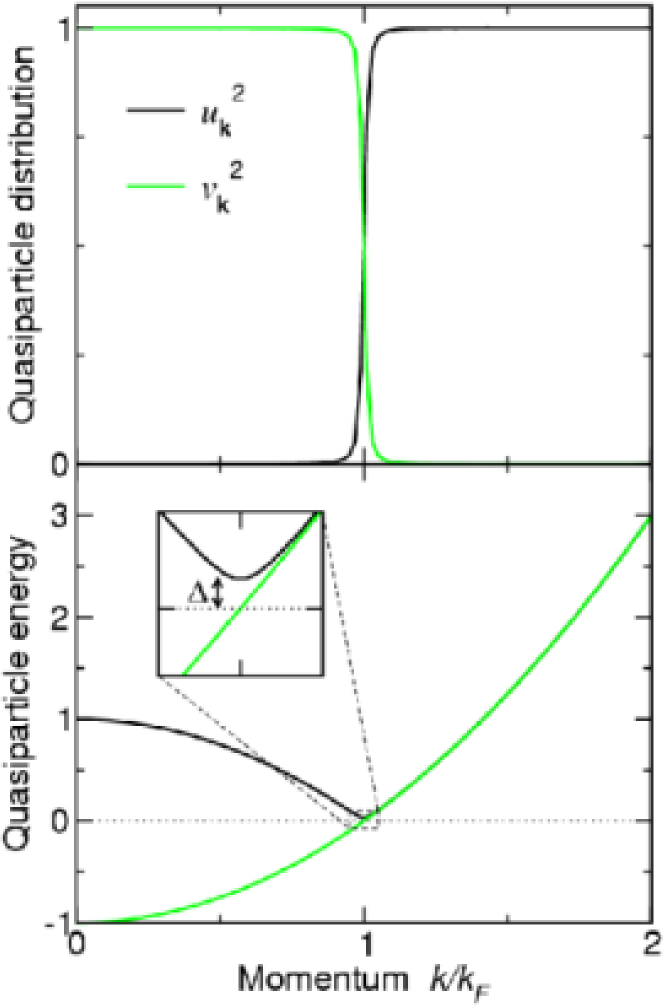
Figure 1.2: bcs results for $\Delta/\mu=0.03$: (Top) Quasiparticle distributions $u_{\bm{k}}^{2}$ (black) and $v_{\bm{k}}^{2}$ (green) and (bottom) quasiparticle energy $E_{\bm{k}}$ (black) compared to the ideal dispersion relation $\epsilon_{\bm{k}}-\mu$ (green) as a function of momentum. The inset is a magnification of the region around the Fermi surface, which shows the existance of a minimum energy value $\Delta$ required to excite the system.

The value of the gap in a symmetric system is also readily calculated starting from Eq. (1.23). As now $E_{A}=0$, we have $E_{\bm{k}}^{+}=E_{\bm{k}}=-E_{\bm{k}}^{-}$, so that $f_{F}(E_{\bm{k}}^{+})-f_{F}(E_{\bm{k}}^{-})=-\tanh(\beta E_{\bm{k}}/2)$. Therefore,

$$\Delta_{\bm{k^{\prime}}}=-\int\frac{\mathrm{d}^{3}k}{(2\pi)^{3}}\,V_{\bm{k^{\prime}}\bm{k}}\,\frac{\Delta_{\bm{k}}}{2E_{\bm{k}}}\tanh\left(\beta\frac{E_{\bm{k}}}{2}\right)\;.$$ (1.25)

This equation is to be solved together with the number equation [compare with Eq. (2.2a)],

$$\rho=\int\frac{\mathrm{d}^{3}k}{(2\pi)^{3}}\,\left[1-\frac{\epsilon_{\bm{k}}-\mu}{\sqrt{(\epsilon_{\bm{k}}-\mu)^{2}+|\Delta|^{2}}}\tanh\left(\beta\frac{E_{\bm{k}}}{2}\right)\right]\;,$$ (1.26)

which accounts for the relationship between the chemical potential and the density of the system. However, in the weak-coupling limit in which we shall be working, one can safely take $\mu=\varepsilon_{F}$. Then Eqs. (1.25) and (1.26) decouple and we only need to worry about the first one.

There are two limiting cases of special interest:

Zero temperature gap $\Delta_{\rm sym}$

When we set $T=1/(k_{B}\beta)=0$, the gap equation reads

$$\Delta_{\bm{k^{\prime}}}=-\int\frac{\mathrm{d}^{3}k}{(2\pi)^{3}}\,V_{\bm{k^{\prime}}\bm{k}}\frac{\Delta_{\bm{k}}}{2E_{\bm{k}}}\;.$$

For a contact interaction of the form $V(\bm{x}-\bm{x^{\prime}})=g\delta(\bm{x}-\bm{x^{\prime}})$, we have $V_{\bm{k^{\prime}}\bm{k}}=g=\mathrm{constant}$, and the integral is ultraviolet divergent. In fact, this formulation of the gap equation has problems for potentials that do not have a well-defined transformation into Fourier space. It is better to resort to the T-matrix, that is the solution to the Lippmann-Schwinger equation and represents the repeated action (summation of ladder diagrams, see Fig. 1.3) of the potential $V$ in a propagating two-body system [Mes99, GP89]

$$\textsf{T}=V+V\frac{1}{E-H+i\varepsilon}V=V+V\frac{1}{E-H_{0}+i\varepsilon}\textsf{T}\;,$$ (1.27)

and is generally well-defined for any interaction. Then, the gap equation reads

$$\Delta_{\bm{k^{\prime}}}=-\int\frac{\mathrm{d}^{3}k}{(2\pi)^{3}}\,\textsf{T}_{\bm{k^{\prime}}\bm{k}}\left(\frac{1}{2E_{\bm{k}}}-\frac{1}{2\epsilon_{\bm{k}}}\right)\Delta_{\bm{k}}\;,$$ (1.28)

which is more convenient for numerial treatment (see Section 2.3).

For dilute systems such as the atomic gases under current experimental research, one has $k_{F}|a|\ll 1$. Therefore, as the integrand in the gap equation is sharply peaked around the Fermi momentum $k_{F}$ in the weak-coupling regime ($\Delta/\mu\ll 1$), we can substitute the momentum-dependent T-matrix by its value at low momenta, which is a constant proportional to the scattering lenght $a$,

$$\textsf{T}_{0}:=\lim_{k^{\prime},k\rightarrow 0}\textsf{T}_{\bm{k^{\prime}}\bm{k}}=\frac{4\pi\hbar^{2}a}{m}\;.$$ (1.29)

Figure 1.3: Diagrammatic representation of the T-matrix: the solid lines represent free propagators, the dashed lines stand for the bare potential $V$ between the two particles, and the wiggle is the T-matrix.

As $\textsf{T}_{0}$ is a constant, it can be pulled out of the integral, and the gap function becomes independent of momentum. With this simplification, and making a change of variables to $x=\epsilon_{\bm{k}}/\mu=\hbar^{2}\bm{k}^{2}/(2m\mu)$ and $d=\Delta/\mu$, the gap equation (1.28) can be rewritten as

$$1 =-\frac{\textsf{T}_{0}}{4\pi^{2}}\int_{0}^{\infty}\mathrm{d}k\,k^{2}\left[\frac{1}{\sqrt{\left(\epsilon_{\bm{k}}-\mu\right)^{2}+\Delta^{2}}}-\frac{1}{\epsilon_{\bm{k}}}\right]$$

$$=-\frac{k_{F}a}{\pi}\int_{0}^{\infty}\mathrm{d}x\,\left[\sqrt{\frac{x}{\left(x-1\right)^{2}+d^{2}}}-\sqrt{x}\right]$$ (1.30)

where we have already integrated the angular variables and used the approximation $\mu\approx\varepsilon_{F}=\hbar^{2}k_{F}^{2}/(2m)$ valid in the weak-coupling limit [FW71, Sch88, PB99]. From this result, we see that the gap in this limit will be a function only of the adimensional parameter $k_{F}a$, irrespective of the specific form of the interparticle potential. Moreover, we shall have a non-vanishing gap only for an attractive interaction, $a<0$, as in the case of the Cooper problem (Section 1.2.1).

A quick, though approximate, evaluation of this integral can be done noting that, for $d\ll 1$, the integrand is sharply peaked around the Fermi surface ($x\approx 1$), which allows us to simplify the first term inside the square brackets taking $x=1$ in its numerator. The resulting integral is analytic, and we obtain

$$\frac{\Delta_{\rm sym}}{\mu}=2\exp\left(\frac{\pi}{2k_{F}a}\right)\qquad(a<0)\;.$$

A more careful evaluation of integral (1.30) gives the well-known result first obtained by Gor’kov and Melik-Barkhudarov [GMB61, PB99]

$$\frac{\Delta_{\rm sym}}{\mu}=\frac{8}{e^{2}}\exp\left(\frac{\pi}{2k_{F}a}\right)\approx 1.083\exp\left(\frac{\pi}{2k_{F}a}\right)\qquad(a<0)\;.$$ (1.31)

Note that the functional dependency on $k_{F}a$ is the same as in the previous expression and only the pre-exponential factor has changed.

Critical temperature $T_{c}$

The critical temperature is defined as the lowest temperature where the gap vanishes. Assuming again a low density, so that the gap is independent of momentum and $\Delta_{\bm{k^{\prime}}}$ cancels with $\Delta_{\bm{k}}$ in the numerator of the gap equation, we can find $T_{c}$ from (1.23) while setting $\Delta=0$ in $E_{\bm{k}}$:

$$1=-g\int\frac{\mathrm{d}^{3}k}{(2\pi)^{3}}\,\frac{1}{2\xi_{\bm{k}}}\tanh\left(\beta_{c}\frac{\xi_{\bm{k}}}{2}\right)\qquad\left(\beta_{c}=\frac{1}{k_{B}T_{c}}\right)\;.$$

This equation is solved in a way similar to that for the zero-temperature gap [GMB61]. The final result is

$$\frac{k_{B}T_{c}}{\mu}=\frac{8e^{\gamma-2}}{\pi}\exp\left(\frac{\pi}{2k_{F}a}\right)\;,$$ (1.32)

where $\gamma=0.5772\cdots$ is Euler’s constant. Note that $T_{c}$ has the same functional dependence on $k_{F}a$ as the gap. Therefore, in the weak-coupling limit, the bcs theory leads to a simple proportionality relationship between the zero-temperature gap and the critical temperature for the superfluid transition, independent of the physical system under study:

$$\frac{k_{B}T_{c}}{\Delta_{\rm sym}}=\frac{e^{\gamma}}{\pi}\simeq 0.567\;.$$ (1.33)

This relationship —which is reasonably well fulfilled by many superconducting metals and alloys [FW71, Kit96], but not by high-temperature superconductors [CSTL05, Bra98]— will allow us to calculate only the zero-temperature gaps. The transition temperatures into the superfluid state for dilute, atomic gases can be obtained then from Eq. (1.33).

1.3 Summary

In this chapter we have introduced the pairing solution for the ground state of a system of interacting fermions. First, we have presented the concept of ‘Cooper pairs’. Then, we have formulated the bcs theory as a solution in terms of Greens’ functions at finite temperature of the interacting Hamiltonian in a self-consistent Hartree-Fock-like approximation, in the general case of a two-component system with density asymmetry, i. e., where the two components may have different densities.

Finally, we have obtained some analytic results for the gap at zero temperature and the critical temperature for the case where both components have equal densities. In chapter 2 we will study how the energy gap, chemical potential and other physical parameters of the sytem are affected when this last condition is not fulfilled.

We remark at this point that an equivalent solution for the Green’s functions for the full interacting Hamiltonian, can be found solving the corresponding Dyson’s equation, which in ($\bm{k},\omega$)-space reads

$$G(\bm{k},\omega)^{-1}=G(\bm{k},\omega)_{0}^{-1}-\Sigma(\bm{k},\omega)\;.$$

Here $G_{0}^{-1}=\omega-\xi_{\bm{k}}+i\,\eta\>{\rm sgn}(\omega)$ is the non-interacting propagator and $\Sigma$ is the self-energy, which has to be determined in order to solve the problem. A further analysis of this approach is beyond the scope of this introductory chapter and can be found in [SMPM05].

Chapter 2 Pairing in density-asymmetric fermionic systems

Politiker, Ideologen, Theologen und Philosophen versuchen immer und immer wieder, restlose L sungen zu bieten, fix und fertig gekl rte Probleme. Das ist ihre Pflicht — und es ist unsere, der Schriftsteller, - die wir wissen, dass wir nichts rest- und widerstandslos kl ren k nnen - in die Zwischenr ume einzudringen.

Heinrich B ll, Nobel lecture

2.1 Introduction

In Chapter 1 we have developed a general formalism to study the bcs pairing mechanism in a system composed of two fermionic species with chemical potentials $\mu_{\uparrow}$ and $\mu_{\downarrow}$, which are not required to be equal. This is a subject of interest in a number of fields of research, such as nuclear physics [MS03b], elementary particles [CN04] and condensed matter physics [Yeh02]. We are mainly interested in the application to dilute, atomic systems where a great deal of work has been devoted since the pioneering contribution of Stoof and coworkers [SHSH96, HFS⁺97], who predicted the possibility to detect a phase transition to a superfluid state in a trapped system of ⁶Li atoms.

After the achievement of Bose-Einstein condensation (BEC) in dilute gases of alkali atoms in 1995 [JILA95, MIT95], an important target in cooling atomic samples was to reach the degenerate regime in a gas of fermionic atoms. Indeed, the mechanism that allowed the production of BECs, known as evaporative cooling, relies intrinsically on the capacity of very cold atoms to quickly re-thermalize when some of them (those with higher energies) are let escape from the trap, see Fig 2.1. At the very low temperatures of interest (of the order of $\mu$K or below), the only remaining interaction in a dilute system are $s$-wave collisions. As these are forbidden between indistinguishable fermions by Pauli’s exclusion principle [GP89, Mes99], this mechanism does not work to cool one-component Fermi gases (e. g., a gas with spin-polarized atoms). For such a system, the loss of very energetic atoms implies, of course, a decrease of the mean energy per particle, but in the absence of a (re)thermalization mechanism, this just means that the system is not in thermal equilibrium, but no redistribution of the remaining atoms in phase space occurs.

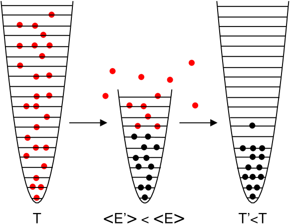
Figure 2.1: Evaporative cooling procedure: in a trapped system of bosons at temperature $T$, the most energetic ones are let escape, thus reducing the mean energy per particle of the remaining ensemble. After rethermalization, the system is at a lower temperature $T^{\prime}<T$.

This limitation can be overcome if the trapped system is not composed just by one kind of fermions. For example, one can trap atoms in two (or more) hyperfine states. In this case, there is no problem for the existence of $s$-wave collisions between atoms belonging to different states and this simultaneous cooling scheme works for such a multi-component fermionic system in the same way as for a bosonic system, as was first shown by DeMarco and Jin at jila [Rice99]. Another possibility is to trap a mixture of bosons and fermions. In this case, the bosons are cooled in the usual way, while the fermions cool down by thermal contact with the bosons, as $s$-wave collisions between them are not forbidden. This mechanism is known as sympathetic cooling and it was first realized by the group of Randy Hulet at Rice University, who reported experiments where a gas of ⁶Li atoms (with fermionic character) was driven to quantum degeneracy by contact with a gas of ⁷Li (bosons) [Rice01].

Since these pioneering works, many groups have produced degenerate Fermi gases around the world [jila, mit, lens, Innsbruck, Paris,…]. One of the main goals of this research has been to create (and detect!) a superfluid made up of atoms, in a sense analog to superfluid helium but with the advantage (in principle) of a much weaker interaction due to the low density of these systems (typically, in the absence of resonant phenomena such as Feshbach resonances, $\rho|a|^{3}\ll 1$, while in helium $\rho a^{3}\sim 1$), which allows for an easier understanding of the physics behind the experiments. In particular, it is possible to use the mean-field bcs theory of pairing in the weak-coupling approximation [SHSH96, HFS⁺97].

In this Chapter, we will study which are the possibilities of having pairing in a two-component fermionic system such as that in [Rice99]. In particular, we will focus on the relevant paper played by the difference in densities of the two components. As we will show, this difference reduces dramatically the size of the energy gap (and, therefore, the expected critical temperature for appearence of superfluidity) when considering pairing between atoms belonging to different species. However, pairing between atoms belonging to the same species can be enhanced by properly adjusting the density of the other species.

2.2 Pairing in $s$-wave

Let us assume a fermionic system composed of two distinct species (which we label $\uparrow$ and $\downarrow$) of equal mass $m$ and with densities $\rho_{\uparrow}$ and $\rho_{\downarrow}$, or equivalently total density $\rho=\rho_{\uparrow}+\rho_{\downarrow}$ and density asymmetry $\alpha=(\rho_{\uparrow}-\rho_{\downarrow})/(\rho_{\uparrow}+\rho_{\downarrow})$. For example, species $\uparrow$ and $\downarrow$ can denote different hyperfine levels of atomic gases, or ‘neutron’ and ‘proton’ in the context of nuclear physics (where one should take into account both the spin and the isospin as internal degrees of freedom of the ‘nucleon’). We also introduce the Fermi momenta $k_{s}\equiv k_{F}^{(s)}=(6\pi^{2}\rho_{s})^{1/3}$, and chemical potentials $\mu_{s}=\hbar^{2}k_{s}^{2}/(2m)$ ($s=\uparrow,\downarrow$), together with $\mu=(\mu_{\uparrow}+\mu_{\downarrow})/2$ and $\delta\mu=(\mu_{\uparrow}-\mu_{\downarrow})/2$.

For simplicity, we will for the moment consider an idealized system where $\uparrow$ and $\downarrow$ particles are interacting via a potential $V$ with $s$-wave scattering length $a$, while direct interactions between like particles $\uparrow$-$\uparrow$ and $\downarrow$-$\downarrow$ are absent [cf. Eq. (1.4) and Fig. 2.2(a)]. We are interested in the situation at very low density, $k_{s}|a|\ll 1$. We have seen in Chapter 1 that, in this limit, the pairing properties of the symmetric system are completely determined by the scattering length or, equivalently, the low-momentum $s$-wave T-matrix, $\textsf{T}_{0}=4\pi\hbar^{2}a/m$. We will now study the general case where the two species can have different densities, and analyze the corresponding pairing gaps generated by this interaction $V$.

Figure 2.2: The two possible lowest-order pairing interactions: (a) Direct $s$-wave interaction between different species. (b) Polarization-induced $p$-wave interaction between like species. V₀ and T₀ are the $s$-wave ($L=0$) bare potential and T-matrix between species $\uparrow$ and $\downarrow$, respectively.

As we did for the symmetric system in Sect. 1.2.3, we must solve the gap equation (1.23),

$$\Delta_{\bm{k^{\prime}}} =\int\frac{\mathrm{d}^{3}k}{(2\pi)^{3}}\,V_{\bm{k^{\prime}}\bm{k}}\,\frac{\Delta_{\bm{k}}}{2E_{\bm{k}}}\left[f_{F}\left(E_{\bm{k}}^{+}\right)-f_{F}\left(E_{\bm{k}}^{-}\right)\right]\>,$$

$$E_{\bm{k}}^{\pm} =E_{A}\pm\sqrt{E_{S}^{2}+|\Delta_{\bm{k}}|^{2}}\;,$$

together with the equations that fix the chemical potential of each species (or, equivalently, $\mu$ and $\delta\mu$) from the values of their densities. These equations can be found again starting from the normal propagators and summing over Matsubara frequencies (see Appendix A):

$$\rho_{\uparrow}(\bm{k}) =\frac{1}{\beta\hbar}\sum_{n}-G_{\uparrow}(\bm{k},\omega_{n})=\frac{1}{2}\left(1+\frac{\xi_{\bm{k}}}{E_{\bm{k}}}\right)f(E_{\bm{k}}^{+})+\frac{1}{2}\left(1-\frac{\xi_{\bm{k}}}{E_{\bm{k}}}\right)f(E_{\bm{k}}^{-})$$

$$=u_{\bm{k}}^{2}f(E_{\bm{k}}^{+})+v_{\bm{k}}^{2}f(E_{\bm{k}}^{-})=u_{\bm{k}}^{2}\left[f(E_{\bm{k}}^{+})-f(E_{\bm{k}}^{-})\right]+f(E_{\bm{k}}^{-})\>,$$ (2.1a)

$$\rho_{\downarrow}(\bm{k}) =\frac{1}{\beta\hbar}\sum_{n}-G_{\downarrow}(\bm{k},\omega_{n})=1-f(E_{\bm{k}}^{+})+u_{\bm{k}}^{2}\left[f(E_{\bm{k}}^{+})-f(E_{\bm{k}}^{-})\right]\>.$$ (2.1b)

These distributions are shown in Fig. 2.3 for $\delta\mu=0.1$ and different values of the gap $\Delta$ to get some physical insight.

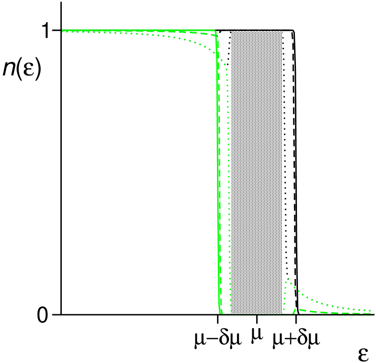
Figure 2.3: bcs momentum distributions of the species $\uparrow$ (black lines) and $\downarrow$ (green lines) in asymmetric matter. The continuous lines stand for the normal matter ($\Delta=0$) distribution, the dashed lines for superfluid matter with $\Delta=0.03\mu$, while the dotted lines show the distributions corresponding to the more coupled case $\Delta=0.07\mu$. [see Eqs. (2.1)]. The shaded area is the ‘forbidden region’ $[\mu-\delta\epsilon,\mu+\delta\epsilon]$ for the case $\Delta=0.07\mu$.

The sharp Fermi surfaces of the non-interacting system smear out for increasing $\Delta$ reflecting the correlations introduced by the pairing interaction. However, this ‘smearing’ hardly penetrates into the region between $\mu_{\downarrow}$ and $\mu_{\uparrow}$ as Pauli’s principle forbids new $\uparrow$ particles to enter there. Thus, the newly formed $\uparrow$-$\downarrow$ pairs need to climb to states $\epsilon_{\bm{k}}>\mu_{\uparrow}$. This has a cost in kinetic energy, which is compensated by the pairing energy gained. Clearly this mechanism cannot sustain arbitrarily large asymmetries, as the kinetic energy investment grows rapidly with the width $\sim 2\delta\epsilon$ of the forbidden region (see below). In fact, one can readily find the total density $\rho$ and density difference $\delta\rho$ to be

$$\rho=\rho_{\uparrow}+\rho_{\downarrow} =\sum_{k}\Big{[}1+\frac{\xi_{\bm{k}}}{E_{\bm{k}}}\left[f_{F}(E_{\bm{k}}^{+})-f_{F}(E_{\bm{k}}^{-})\right]\Big{]}\>,$$ (2.2a)

$$\delta\rho=\rho_{\uparrow}-\rho_{\downarrow} =\sum_{k}\left[f_{F}(E_{\bm{k}}^{+})+f_{F}(E_{\bm{k}}^{-})-1\right]\>.$$ (2.2b)

At zero temperature, $f_{F}(E)=\Theta(-E)$ and, therefore,

$$f_{F}(E_{\bm{k}}^{+})-f_{F}(E_{\bm{k}}^{-}) =-\Theta(E_{\bm{k}}^{+})\>,$$

$$f_{F}(E_{\bm{k}}^{+})+f_{F}(E_{\bm{k}}^{-})-1 =\Theta(-E_{\bm{k}}^{+})\>,$$

where we used the fact that $\Theta(x)=1-\Theta(-x)$. From the second equation we see that the unpaired particles are to be found in the energy interval $[\mu-\delta\epsilon,\mu+\delta\epsilon]$, with $\delta\epsilon=\sqrt{{\delta\mu}^{2}-{\Delta}^{2}}$ ($\approx\delta\mu$ for $\Delta<\mu$), which does not contribute to the pairing interaction, as indicated by the shaded area in Fig. 2.3. This leads to a rapid decrease of the resulting gap when increasing the asymmetry.

In the weak-coupling case, $\Delta\ll\delta\epsilon\ll\mu$, which is adequate in the low-density limit, the momentum distributions of the two species are anyhow very sharp and one obtains from Eqs. (2.2)

$$\rho =\int\frac{\mathrm{d}^{3}k}{(2\pi)^{3}}\,\left[1+\frac{\xi_{\bm{k}}}{E_{\bm{k}}}\left(1-\Theta\left(-E_{\bm{k}}^{+}\right)\right)\right]$$

$$=\frac{1}{4\pi^{2}}\left(\frac{2m\mu}{\hbar^{2}}\right)^{3/2}\left\{\left(\int_{0}^{1+\delta x}+\int_{1+\delta x}^{\infty}\right)\mathrm{d}x\,\sqrt{x}\right.$$

$$\qquad\left.-\int_{0}^{1-\delta x}\mathrm{d}x\,\sqrt{x}\frac{x-1}{\sqrt{(x-1)^{2}+d^{2}}}-\int_{1+\delta x}^{\infty}\mathrm{d}x\,\sqrt{x}\frac{x-1}{\sqrt{(x-1)^{2}+d^{2}}}\right\}$$

$$\approx\frac{1}{2\pi^{2}}\left(\frac{2m}{\hbar^{2}}\right)^{3/2}\frac{2}{3}\mu^{3/2}$$

and

$$\delta\rho =\int\frac{\mathrm{d}^{3}k}{(2\pi)^{3}}\,\Theta\left(\delta\mu-\sqrt{(\epsilon_{\bm{k}}-\mu)^{2}-|\Delta|^{2}}\right)$$

$$=\frac{1}{4\pi^{2}}\left(\frac{2m\mu}{\hbar^{2}}\right)^{3/2}\int_{0}^{\infty}\mathrm{d}x\,\sqrt{x}\,\Theta\left(\delta x-\sqrt{(x-1)^{2}+d^{2}}\right)$$

$$\approx\frac{1}{2\pi^{2}}\left(\frac{2m}{\hbar^{2}}\right)^{3/2}\mu^{1/2}\delta\epsilon\;,$$

where we used the shortening $\delta x=\delta\epsilon/\mu$ and $d=\Delta/\mu$, and the fact that $\delta\mu\ll\mu$. Therefore,

$$\alpha=\frac{\delta\rho}{\rho}\approx\frac{3}{2}\frac{\delta\epsilon}{\mu}\ll 1\>,$$ (2.3)

i. e., the width of the forbidden region $\delta\epsilon$ is directly proportional to the density asymmetry $\alpha$. Analyzing in a similar way the gap equation, one can obtain these relationships involving the parameter $\delta\epsilon$ [SHSH96, SAL97, SL00],

$$\delta\mu+\delta\epsilon={\rm const.}=\Delta_{\rm sym}\quad\Leftrightarrow\quad\Delta^{2}=\Delta_{\rm sym}^{2}-2\Delta_{\rm sym}\delta\epsilon\>,$$

where $\Delta_{\rm sym}$ is the gap in symmetric matter of the same density $\rho$ [Eq. (1.31)]. Altogether, we can write the gap as a function of the asymmetry thus:

$$\frac{\Delta(\alpha)}{\Delta_{\rm sym}}=\sqrt{1-\frac{4\mu}{3\Delta_{\rm sym}}\alpha}\;.$$ (2.4)

It vanishes at $\alpha_{\rm max}^{BCS}=3\Delta_{\rm sym}/(4\mu)$, which is an exponentially small number in the weak-coupling limit $k_{F}|a|\ll 1$. Therefore, for very small asymmetries already, pairing generated by the direct interaction between different species becomes impossible according to the bcs theory. However, this limitation can be partially overcome, as we will see in chapter 3.

2.3 Numerical results

2.3.1 The algorithm

Let us now present our numerical procedure to solve the gap equation and check the results with the previous analytical calculations. We start rescaling all energies in units of the mean chemical potential,

$$x =\epsilon_{\bm{k}}/\mu d =\Delta/\mu \delta x =\delta\epsilon/\mu$$

$$E_{x} =E_{\bm{k}}/\mu E_{x}^{\pm} =-\frac{\delta\mu}{\mu}\pm E_{x} x^{\pm} =E_{\bm{k}}^{\pm}/\mu\>,$$

Assuming a constant value for $V_{\bm{k^{\prime}}\bm{k}}=g$, so that the gap function will not depend on momentum, we rewrite the gap equation as

$$1 =g\frac{\left(2m\right)^{3/2}}{8\pi^{2}\hbar^{3}}\sqrt{\mu}\int_{0}^{\infty}\mathrm{d}x\,\sqrt{x}\frac{1}{E_{x}}\left[f_{F}\left(\mu x^{+}\right)-f_{F}\left(\mu x^{-}\right)\right]\>.$$

To avoid a possible divergence in the gap equation due to the use of a contact potential, we resort to the T-matrix as in Sect. 1.2.3 (see also [MPS98]). We get for the general low-density, asymmetric case

$$1=\frac{a}{\pi}\sqrt{\frac{2m\mu}{\hbar^{2}}}\int_{0}^{\infty}\mathrm{d}x\,\sqrt{x}\left\{\frac{1}{E_{x}}\left[f_{F}\left(\mu x^{+}\right)-f_{F}\left(\mu x^{-}\right)\right]+\frac{1}{x}\right\}\>,$$ (2.5)

where we used $\textsf{T}_{0}=4\pi\hbar^{2}a/m$ for a low-density system. Regarding the densities, they are given by integrating Eqs. (2.1). We present below our numerical results for the solution of equations (2.1) and (2.5) obtained in the following way:

1. Introduce an ‘effective Fermi momentum’ $k_{\mu}$ through the chemical potential, $\mu\equiv\hbar^{2}k_{\mu}^{2}/(2m)$.

2. Define the functions

   $$f =\frac{\pi}{k_{\mu}a}-\int_{0}^{\infty}\mathrm{d}x\,\sqrt{x}\left\{\frac{1}{E_{x}}\left[f_{F}\left(\mu x^{+}\right)-f_{F}\left(\mu x^{-}\right)\right]+\frac{1}{x}\right\}$$

   $$g =\frac{4\pi^{2}\rho_{\uparrow}}{k_{\mu}^{3}}-\int_{0}^{\infty}\mathrm{d}x\,\sqrt{x}\left\{u_{x}^{2}\left[f_{F}(\mu x^{+})-f_{F}(\mu x^{-})\right]+f_{F}(\mu x^{-})\right\}$$

   $$h =\frac{4\pi^{2}\rho_{\downarrow}}{k_{\mu}^{3}}-\int_{0}^{\infty}\mathrm{d}x\,\sqrt{x}\left\{1-f_{F}(\mu x^{+})+u_{x}^{2}\left[f_{F}(\mu x^{+})-f_{F}(\mu x^{-})\right]\right\}$$

   with $u_{x}^{2}=[1+(x-1)/E_{x}]/2$. These are functions of the gap $d$ (through $E_{x}$) and the chemical potentials $\mu_{\uparrow}$ and $\mu_{\downarrow}$ (through $\mu$, $k_{\mu}$ and $x^{\pm}$). They must be zero at the solution of Eqs. (2.1) and (2.5).

3. Assume some initial values $d=d^{(0)}$, $\mu_{\uparrow\downarrow}=\mu_{\uparrow\downarrow}^{(0)}$. As we work at fixed total density $\rho$ and density asymmetry $\delta\rho=\rho\alpha$, we have used these guesses:

   $$d^{(0)} =\frac{\Delta(\alpha)}{\mu^{(0)}}\quad\text{[cf. Eq.\leavevmode\nobreak\ (\ref{eq:sgap})],} \mu_{\uparrow\downarrow}^{(0)} =\varepsilon_{F}\left(1\pm\alpha\right)^{2/3}\>.$$

   with $\varepsilon_{F}=\hbar^{2}\left(3\pi^{2}\rho\right)^{2/3}/(2m)$.

4. Insert these values into $f$ and find (e. g., by a Newton-Raphson method) a zero of $f$ as a function solely of $d$. Call this zero $d^{(1)}$.

5. Insert $d^{(1)}$ and $\mu_{\uparrow\downarrow}^{(0)}$ into $g$, and find a zero of $g$ as a function of solely $\mu_{\uparrow}$. Call this zero $\mu_{\uparrow}^{(1)}$.

6. Insert $d^{(1)},\leavevmode\nobreak\ \mu_{\uparrow}^{(1)}$ and $\mu_{\downarrow}^{(0)}$ into $h$, and find a zero of $h$ as a function of solely $\mu_{\downarrow}$. Call this zero $\mu_{\downarrow}^{(1)}$.

7. If the new values for $d$ and $\mu_{\uparrow\downarrow}$ make $|f|,\leavevmode\nobreak\ |g|$ and $|h|$ smaller than a certain tolerance $\varepsilon$ (in our calculations, typically $\varepsilon\sim 10^{-4}$), take them as the solution. Otherwise, go back to step 4 and try again until convergence is reached.

2.3.2 Symmetric case

First of all, in order to test our code, we analyze the dependence of the gap and the chemical potential for the symmetric case, $k_{\uparrow}=k_{\downarrow}\equiv k_{F}$, at low temperatures. We fix $T=0.1T_{c}$, with $T_{c}$ the bcs weak-coupling prediction for the critical temperature as given by Eq. (1.33). The results that we obtain are plotted in Fig. 2.4. In the left panel we show with circles the calculated variation of the energy gap $\Delta$ with the coupling $k_{F}|a|$. For comparison, the solid curve is the bcs prediction at low-density, Eq. (1.31). We see that the agreement is very good for all $k_{F}|a|<1$, and only deviates slightly for $k_{F}|a|\gtrsim 1.3$. The ‘effective’ Fermi momentum $k_{\mu}=\sqrt{2m\mu}/\hbar$ (normalized to the non-interacting Fermi momentum $k_{F}=\sqrt{2m\varepsilon_{F}}/\hbar$) is plotted in the right panel also as a function of the coupling. In this case, we find $k_{\mu}\approx k_{F}$ for $k_{F}|a|\leq 1$, with a smooth decrease that becomes more pronounced above this value of the coupling. This is a signal of the increasing modification of the system with respect to the non-interacting one for such large couplings. In fact, for these values of $k_{F}|a|$ the mean-field bcs theory is not adequate, and more sophisticated methods need to be used [HKCW01, OG02, BY04, FS04, PPS04, CSTL05]. Therefore, we shall not work in the following in this strong-coupling regime.

.

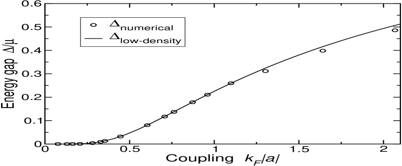
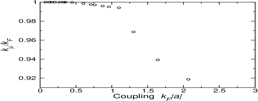
Figure 2.4: Solution of the bcs equations for a temperature $T=0.1T_{c}$ and varying coupling: (Left) Numerical solution for the gap $\Delta$ as a function of the coupling and prediction of bcs at low density, Eq. (1.31). (Right) Effective Fermi momentum $k_{\mu}$ as a function of the coupling. .

Next we analyze the temperature dependence of the same quantities above. To satisfy the weak-coupling condition just discussed, we fix the density to $\rho=2\times 10^{-12}$ cm^-3, so that $k_{F}|a|=0.445524797<1$. The results are shown in Fig. 2.5. In the left panel, the energy gap [divided by the zero-temperature value (1.31)] is plotted as a function of the reduced temperature $T/T_{c}$, with $T_{c}$ given again by Eq. (1.33). Our numerical results are shown with empty circles, while the two lines are the analytical curves of the bcs model (see Ref. [FW71], p. 449) at low and ‘high’ temperatures:

$$\Delta_{\rm low\leavevmode\nobreak\ T} =\Delta_{\rm sym}\left[1-\sqrt{2\pi\frac{k_{B}T}{\Delta_{\rm sym}}}e^{-\Delta_{\rm sym}/k_{B}T}\right]\>, T/T_{c}\ll 1\,,$$

$$\Delta_{\rm high\leavevmode\nobreak\ T} =\sqrt{\frac{8\pi^{2}}{7\zeta(3)}}k_{B}T_{c}\left(1-\frac{T}{T_{c}}\right)^{1/2}\>, (T_{c}-T)/T_{c}\ll 1\,.$$

Both predictions agree well with the data in the corresponding ranges of validity. More specifically, the low-temperature curve is very close to the calculated values for $T/T_{c}\lesssim 0.5$, while the ‘high’-temperature one is valid for $T/T_{c}\gtrsim 0.85$.

.

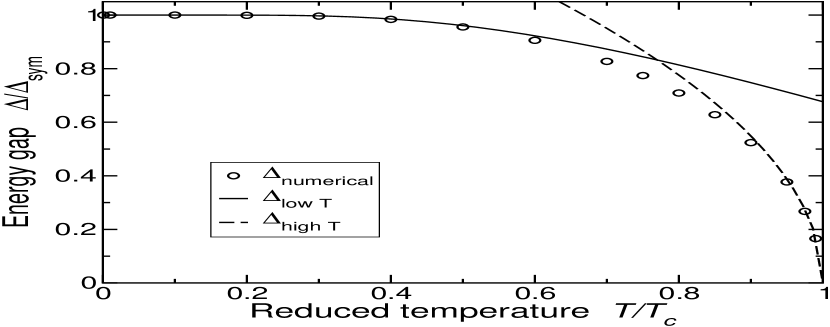
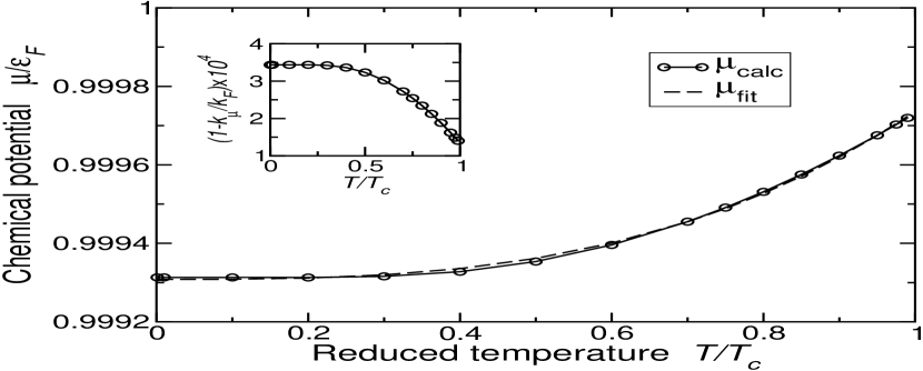
Figure 2.5: Solution of the bcs equations at finite temperature for a fixed density $\rho=2\times 10^{-12}$ cm^-3: energy gap (left) and chemical potential (right) vs. reduced temperature $T/T_{c}$. See the text for details on the notation. .

Regarding the chemical potential (shown by the circles and the solid curve, which is a guide to the eye), it is always very similar to the non-interacting one, i. e., $\varepsilon_{F}$. However, the weak attraction between the fermions results in a slight reduction of $\mu$, that diminishes when approaching the critical temperature, where the gap is expected to vanish (but the system is still interacting, hence the difference between $\mu$ and $\varepsilon_{F}$). The dependence of $\mu$ on temperature can be well fitted by

$$\mu=\mu(T=0)\left[1-\gamma\left({T}/{T_{c}}\right)^{3}\right]\>,$$

as shown by the dashed curve in the figure. Here $\mu(T=0)$ is the chemical potential at zero temperature, and $\gamma$ an adjustable parameter, for which we found the best value $\gamma=4.28\times 10^{-4}$ ($\chi^{2}_{\rm fit}=3.06\times 10^{-10}$). In an equivalent plot, the inset to the right figure shows the variation of $1-k_{\mu}/k_{F}$ as a function of temperature.

2.3.3 Asymmetric case

After this short overview of the symmetric case, we will study the dependence of the gap on the density asymmetry $\alpha=\delta\rho/\rho$ in order to check numerically Eq. (2.4). We consider $T=0$ and again the density $\rho=2\times 10^{12}$ cm^-3 ($k_{F}|a|\sim 0.4$) as we have seen in the previous paragraph that it is well into the bcs validity regime. Our results are summarized in Fig. 2.6. On the left panel, we show how the energy gap $\Delta$ varies with increasing asymmetry $\alpha$. The circles are the calculated data, while the line corresponds to Eq. (2.4), with the $\Delta_{\rm sym}$ given by Eq. (1.31); the dashed vertical line indicates the expected asymmetry $\alpha_{\rm max}^{BCS}=2.4\%$ where the gap will vanish. The agreement between the calculation and the expected behavior is excellent for all asymmetries, even very close to this limiting asymmetry.

.

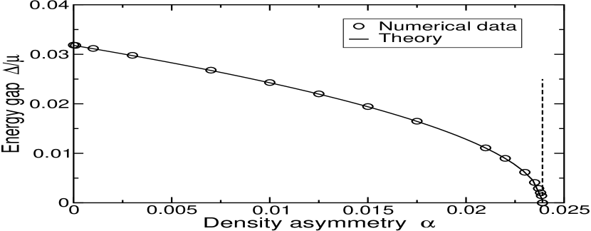
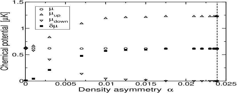
Figure 2.6: Solution of the bcs equations for a fixed density $\rho=2\times 10^{-12}$ cm^-3 at zero temperature as a function of the density asymmetry $\alpha$. (Left) Energy gap; (Right) Chemical potentials: total $\mu$ (circles), $\mu_{\uparrow}$ (triangles up), $\mu_{\downarrow}$ (triangles down) and difference $\delta\mu$ (filled squares). .

On the right panel, we show, for comparison with the symmetric case, the dependence of the mean chemical potential $\mu$ together with the chemical potentials $\mu_{\uparrow\downarrow}$ and $\delta\mu$. We see that $\mu$ depends only very weakly on $\alpha$, as compared to what happens with $\mu_{\uparrow}$ and $\mu_{\downarrow}$. These start being equal in the symmetric case, and separate in an approximately linear way for increasing $\alpha$ until $\alpha\approx 0.01$, where they ‘saturate’ to the values that they will have for $\alpha=\alpha_{\rm max}^{BCS}$. As one would expect, an analogous behavior is followed by $\delta\mu$.

As a conclusion, we have checked numerically the expected behavior of the gap for the $s$-wave solution to the coupled equations determining the gap and the densities. In particular, we have seen that the mean chemical potential is essentially equal to the non-interacting value $\varepsilon_{F}$ and that the gap vanishes for very small asymmetries. At finite temperatures, as one would expect, we have checked also that the gap decreases, and so the maximum asymmetry that would allow pairing is even smaller.

2.4 Pairing in $p$-wave

Therefore, for larger asymmetries only pairing between identical fermions can take place. In this case, Pauli’s exclusion principle demands the paired state to be antisymmetric under exchange of the particles, which for spin-polarized atoms means that they must be in a state of odd angular momentum $L$. The leading contribution to the interaction will be the $p$-wave one.

We discuss in the following the pairing of $\uparrow$-particles mediated by the polarization interaction due to particles pertaining to species $\downarrow$ as shown in Fig. 2.2(b). We will check below that this contribution is dominant over the direct $p$-wave $\uparrow$-$\uparrow$ interaction at low density. Quantitatively the relevant interaction kernel reads [GMB61, HPSV00, SPR01, KC88, BKK96]

$$\left\langle\bm{k^{\prime}}\left|\Gamma_{\uparrow}\right|\bm{k}\right\rangle=\frac{\Pi_{\downarrow}(|\bm{k}^{\prime}-\bm{k}|)}{2}\textsf{T}_{0}^{2}\>.$$ (2.6)

The factor 1/2 corrects for the fact that conventionally the Lindhard function (pertaining to species $\downarrow$),

$$\Pi_{\downarrow}(q)=-\frac{mk_{\downarrow}}{\pi^{2}}\left[\frac{1}{2}+\frac{1-x^{2}}{4x}\ln\left|\frac{1+x}{1-x}\right|\right]\ ,\quad x=\frac{q}{2k_{\downarrow}}\>,$$ (2.7)

contains a factor two for the spin orientations [FW71], which is not present in our case as we are dealing with fermions without internal degrees of freedom.

One can see that $\Pi_{\downarrow}<0$. Therefore, the effective interaction is always attractive, irrespective of the sign of $a$ [FL68]. This is due to the absence of exchange diagrams, which makes $\Pi_{\downarrow}$ attractive in contrast to the case of one species, where the polarization effects reduce the $s$-wave bcs gap by a factor $(4e)^{1/3}\approx 2.2$ even in the low-density limit, where one would naively expect them to be negligible. [GMB61, HPSV00, SPR01]. One can therefore assert that, even in the limit $k_{F}\rightarrow 0$ bcs is not such a good aproximation, as it disregards these higher-order interactions.

Now we project out the $p$-wave (i. e., $L=1$) contribution of the interaction with the Legendre polynomial $P_{1}(z)=z$, with $z=\bm{\widehat{k}}^{\prime}\cdot\bm{\widehat{k}}$ the cosine of the angle between the in- and out-going relative momenta, which in the range of the weak-coupling approximation we can take on the Fermi surface [KC89, EMBK00]

$$\Gamma^{(L=1)}_{\uparrow}(k_{\uparrow},k_{\uparrow})=\frac{\textsf{T}_{0}^{2}}{2}\,\frac{1}{2}\!\int_{-1}^{+1}\!dz\,z\,\Pi_{\downarrow}(\sqrt{2(1-z)}k_{\uparrow})\>.$$

The integral of the Lindhard function can be evaluated making use of the result [SPR01]

$$\int_{0}^{Z}\mathrm{d}x\,x^{3}\Pi(x)=\frac{1}{12}\left[2\ln|1-Z^{2}|+(5-3Z^{2})Z^{3}\ln\left|\frac{1+Z}{1-Z}\right|+2Z^{2}+6Z^{4}\right]$$

resulting in

$$\Gamma^{(1)}_{\uparrow}(k_{\uparrow},k_{\uparrow})=-\frac{8a^{2}k_{\downarrow}}{m}\frac{2\ln 2-1}{5}g\Big{(}\frac{k_{\uparrow}}{k_{\downarrow}}\Big{)}\>,$$

where we introduced

$$g(y)=-\frac{1}{6(2\ln 2-1)y^{4}}\Big{[}(4-10y^{2})\ln\left|1-y^{2}\right|\\ -(5+y^{2})y^{3}\ln\left|\frac{1+y}{1-y}\right|+4y^{2}+2y^{4}\Big{]}\>.$$ (2.8)

This function is normalized in symmetric matter, $g(1)=1$, and it is plotted in Fig. 2.7(a).

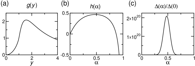
Figure 2.7: (a,b) The functions $g$ and $h$, appearing in Eqs. (2.8) and (2.12), respectively. (c) The variation of the gap with asymmetry, Eq. (2.11), for a density parameter $u=100$. .

It is customary to replace the numerical factor $(2\ln 2-1)/5$ in Eq. (2.4) by its approximate value 1/13.

We use now the general result for the (angle-averaged) $L$-wave pairing gap [FL68, AM61, KL65],

$$\Delta_{L}(k_{\uparrow})\rightarrow c_{L}\,\mu_{\uparrow}\exp\!\left[\frac{2\pi^{2}\hbar^{2}}{mk_{\uparrow}\textsf{T}_{L}(k_{\uparrow},k_{\uparrow})}\right]\>,$$ (2.9)

with $\textsf{T}_{L}$ the $L$-wave projection of the relevant interaction and $c_{L}$ a constant of order unity. Considering that for a pure polarization interaction $\Gamma_{L}$ the leading order in density is $\textsf{T}_{L}=\Gamma_{L}$, we get

$$\Delta_{1}(k_{\uparrow})=c_{1}\frac{k_{\uparrow}^{2}}{2m}\exp\!\left[-\frac{13(\pi/2)^{2}}{a^{2}k_{\uparrow}k_{\downarrow}g(k_{\uparrow}/k_{\downarrow})}\right]\>.$$ (2.10)

Taking into account the dependence of this expression on the two Fermi momenta $k_{\uparrow\downarrow}=[3\pi^{2}\rho(1\pm\alpha)]^{1/3}$, the final result for the variation of the pairing gap with asymmetry $\alpha$ and total density $\rho$ can be cast in the form

$$\frac{\Delta_{1}(\rho,\alpha)}{\Delta_{1}(\rho,0)}=(1+\alpha)^{2/3}\exp\left[u(\rho)h(\alpha)\right]$$ (2.11)

with

$$h(\alpha)=1-\frac{1}{(1-\alpha^{2})^{1/3}g\left[((1+\alpha)/(1-\alpha))^{1/3}\right]}$$ (2.12)

and the density parameter

$$u(\rho)=13\left(\frac{\pi}{2{k_{F}}a}\right)^{2},\quad{k}_{F}\equiv(3\pi^{2}\rho)^{1/3}\>.$$

The function $h(\alpha)$ is displayed in Fig. 2.7(b), where $\alpha=1$ corresponds to pure $\uparrow$-matter. One notes a maximum at $\alpha_{\mathrm{opt}}\approx 0.478$ with an expansion $h(\alpha)\approx 0.465-1.343(\alpha-0.478)^{2}$.

At the optimal asymmetry, the gap is enhanced with respect to that of the symmetric case [$h(0)=0$] by a factor $e^{0.465u}\approx 10^{0.20u}$. In the low-density limit $u\rightarrow\infty$ this represents an enormous amplification at finite asymmetry. Around this peak, the variation of the gap with asymmetry is well described by a Gaussian with width $\sigma=1/(1.64\sqrt{u})$. As an illustration of this effect, Fig. 2.7(c) shows the ratio (2.11) for a value of the density parameter $u=100$ (corresponding to $k_{F}|a|\approx 0.57$). As expected from the previous discussion, a peak of the order of $10^{20}$ is observed, that becomes rapidly more pronounced and narrower with decreasing density $\rho$ (increasing $u$), although of course at the same time the absolute magnitude of the gap decreases strongly with decreasing density: $\Delta_{1}(\rho,0)\propto\exp(-u)$ [Eq. (2.10)].

Let us now briefly discuss higher-order effects, namely contributions of order $(k_{F}a)^{3}$ in the denominator of the exponent of Eq. (2.10). There are two principal sources of such effects, which are shown diagramatically in Fig. 2.8.

Figure 2.8: Third-order diagrams in a one-component system: (a) Direct $p$-wave interaction, (b) Polarization contribution.

The first one, Fig. 2.8(a), is the direct $p$-wave interaction [YM99] between like species that we have neglected before. Parametrizing the low-density $p$-wave T-matrix in the standard form $\textsf{T}_{1}(k,k^{\prime})\approx 4\pi a_{1}^{3}kk^{\prime}/m$, where $a_{1}^{3}$ is the $p$-wave scattering volume, leads to a bcs gap [YM99]

$$\frac{\Delta_{1}}{\mu_{\uparrow}}=\frac{8}{e^{8/3}}\exp\!\left[\frac{\pi}{2(k_{\uparrow}a_{1})^{3}}\right]\>.$$ (2.13)

where we have explicitly determined the prefactor of the exponential. This gap is much smaller than the $\downarrow$-mediated one for $\{|a|,|a_{1}|\}\ll k_{\uparrow}^{-1}$, which justifies the fact that we neglect this effect in the previous calculation. However, around a $p$-wave Feshbach resonance, where $|a_{1}|\gg|a|$, this effect might be important, even though this kind of pairing has not been observed in the experiments that explored the $p$-wave resonance of ⁴⁰K in the hyperfine state $|F=9/2,m_{F}=-/2\rangle$ [JILA03c] or ⁶Li in $|F=1/2\rangle$ [ENS04b] (see also [Boh00] for theoretical calculations of the position of the resonances, and [Stan00, Inns03] for experiments on bosonic cesium).

The second type of third-order contributions are polarization effects involving the $s$-wave scattering length $a$. In contrast to the case of a one-component system, where there are several relevant diagrams, in the present two-component system only one diagram exists, Fig. 2.8(b). Unfortunately it can only be computed numerically, which we have not attempted.

Finally, to fourth order, there is a large number of diagrams contributing to the interaction kernel. Moreover, at this order it is also necessary to take into account retardation effects, i. e., the energy dependencies of gap equation, interaction kernel, and self-energy need to be considered [AG92]. All this can only be done numerically and was performed in Ref. [EMBK00] for the case of a one-component system.

In any case, the existence of higher-order corrections will not alter the main conclusions drawn so far, namely the presence of a strongly peaked Gaussian variation of the gap with asymmetry. They may, however, shift this peak to a different density-dependent location, and also modify the absolute size of the gap. Furthermore, we must note again that the perturbative approach that we have followed is clearly limited to the low-density range $k_{F}|a|<1$. For larger couplings, different theoretical methods are required, which is an interesting field of current investigation [BB73, AB87, HKCW01, OG02, BY04, PPS04, FDS04, CSTL05].

2.5 Summary

In this chapter, we have studied the possibility of pairing in a system composed of two distinct fermionic species, assuming that the direct $p$-wave interaction between like species can be neglected. First, we have studied analytically the gap produced by a direct, attractive, $s$-wave interaction between different species. We have shown that it produces a gap $\sim\exp\!\left[{\pi/2k_{F}a}\right]$ [Eq. (1.31)] only for very small asymmetries between the densities of the two species, $\alpha\lesssim\Delta_{\rm sym}/\mu$, Eq. (2.4). We have numerically checked this behavior, and we have seen that, in fact, the maximum asymmetry decreases with temperature.

However, a $p$-wave attraction between two fermions of the same species produced by a polarization of the medium of the other species, can give rise to pairing over the whole range of asymmetry. In practice a sharp Gaussian maximum around $\alpha\approx 0.478$ ($\rho_{\uparrow}/\rho_{\downarrow}\approx 2.83$, $k_{\uparrow}/k_{\downarrow}\approx$ 1.41) appears. Unfortunately, the absolute magnitude of this gap is rather small, as it depends strongly on the density of the system, $\sim\exp\!\left[-13({\pi/2k_{F}a})^{2}\right]$, which we assumed low in order to be in the range of validity of the bcs mean-field approach.

We argue that higher-order corrections may modify quantitatively but not qualitatively these general features.

The experimental observation of both types of pairing in dilute, atomic vapors is expected to be difficult. For the case of $p$-wave pairing due to the extremely small size of the expected gap, which translates into a very low transition temperature [remember Eq. (1.33)], which is difficult to reach experimentally (see Sect. 2.1). For the $s$-wave case, the nearly perfect symmetry that is required poses a difficult experimental challenge. However, the present possibility to transform a two-component Fermi gas into a molecular gas by crossing a Feshbach resonance [JILA04b, Inns04] opens the door to create a perfectly symmetric system by removing the atoms not converted into molecules and, then, going back across the resonance, forming again a two-component fermionic system, now with well-balanced populations. Up to now, the experiments have focused on the strongly-interacting regime $k_{F}|a|\gtrsim 1$ where superfluidity might arise at higher temperatures. Once this has been succesfully achieved [MIT05], one could imagine to go further to the weak-coupling regime and transfer atoms in a controled way from one hyperfine state to the other by RF pulses, which would allow a precise experimental check of Eq. (2.4) in case low enough temperatures were achieved.

Chapter 3 Pairing with broken space symmetries: loff vs. dfs

Bill Waterson, Calvin and Hobbes

3.1 Introduction

In chapter 1 we introduced the bcs theory for pairing in a fermionic system. We showed that this theory predicts a phase transition into a superfluid state for temperatures of the order of $\Delta_{\rm sym}/k_{B}$, where in the weak-coupling regime $k_{F}|a|\ll 1$ [see Eq. (1.31)]

$$\frac{\Delta_{\rm sym}}{\mu}=\frac{8}{e^{2}}\exp\left(\frac{\pi}{2k_{F}a}\right)\>.$$ (3.1)

Stoof and coworkers were the first to point out that this result, when applied to dilute systems of ⁶Li, predicts relatively large gaps for moderate densities (e. g., $\rho\sim 10^{12}$ cm^-3) due to the large (negative) value of the $s$-wave scattering length of this species, $a=-2160a_{B}$ ($a_{B}\approx 0.53$ Å is Bohr’s radius). These large gaps would translate in transition temperatures of the order of nanokelvin and, therefore, possibly within experimental reach in a short time after their proposal in 1996 [SHSH96]. Regarding the problem on the density asymmetry between the two species to pair, they also pointed out ‘that the most favorable condition for the formation of Cooper pairs is that both densities are equal’. Then, they solved the gap equation in this most favorable situation, for a trapped system of ⁶Li atoms using local density approximation (lda) [HFS⁺97].

In chapter 2 we have carefully analyzed why a two-component symmetric system will always have $s$-wave gaps larger than asymmetric systems. Besides, we have also shown that these $s$-wave gaps are non-vanishing, within standard bcs theory, for quite a narrow window of density asymmetries $\alpha$. For $\alpha>\alpha_{\rm max}^{BCS}=3\Delta_{\rm sym}/(4\mu)$ [cf. Eq. (2.4)], only $p$-wave pairing between atoms in the same hyperfine state seems possible. However, we have seen that the size of this gap is rather small, and in fact it is difficult to expect this phase to be detected experimentally. Now we will explore another way of overcoming the density-asymmetry problem. To this end, we solve the gap equation on a wider space of functions, allowing for more complex structures than the typical rotationally-symmetric order parameter found in chapters 1 and 2.

In references [MS02, MS03b] it was shown that for nuclear matter at saturation density —which is a strongly coupled system ($\Delta_{0}/\mu\sim 0.3$)— a superconducting state featuring elliptically deformed Fermi surfaces (dfs) was preferable to the spherically symmetric bcs state. Following these ideas, we propose here to explore the weak-coupling regime of this theory in connection with current experiments with ultracold, dilute systems.

It has been known for a long time that the homogeneous bcs phase can evolve into the Larkin-Ovchinnikov-Fulde-Ferrell (loff) phase [LO64, FF64], which can sustain asymmetries $\alpha>\alpha_{\rm max}^{BCS}$ by allowing the Cooper pairs to carry a non-vanishing center-of-mass momentum. Note that, even though both the loff and the dfs phases break the global space symmetries, they do it in fundamentally different ways: the loff phase breaks both rotational and translational symmetries due to the finite momentum of the pairs’ condensate. On the contrary, the dfs phase breaks only the rotational symmetry [from O(3) down to O(2)]. We remark also that, after so many years since its proposal, only very recently some experimental evidences of the detection of the loff phase have been reported in the heavy-fermion compound CeCoIn₅ (see [RFM⁺03, BMC⁺03, WKI⁺04, KSK⁺05, MAT⁺05]). In this sense, it is interesting to note that atomic systems offer a novel setting for studying the loff phase under conditions that are more favorable than those in solids (absence of lattice deffects, access to the momentum distribution in the system through time-of-flight experiments) as explored in [Com01, CM02, MC03, MMI05, Yan05]. These systems also offer the possibility of novel realizations of the loff phase which for example invoke $p$-wave anisotropic interactions [Com01]. There has been also much interest in the loff phase in connection with hadronic systems under extreme conditions where the interactions are mediated by the strong force, see [ABR01, Sed01, BR02, CN04]. In this context no experimental detection of this phase has been reported yet.

We note that another possible configuration for a density-asymmetric system is the phase separation of the superconducting and normal phases in real space, such that the superconducting phase contains particles with the same chemical potentials (i. e., it is symmetric), while the normal phase remains asymmetric, see [Bed02, BCR03, Cal04]. The description of such an heterogeneous phase requires knowledge of the poorly known surface tension between superconducting and normal phases, and will not be attempted here.

We shall compare below the realizations of the dfs and loff phases in an ultracold gas of ⁶Li atoms where the hyperfine states $|\!\!\uparrow\rangle=|F=3/2,m_{F}=3/2\rangle$ and $|\!\!\downarrow\rangle=|3/2,1/2\rangle$ are simultaneously trapped. Here, $F$ denotes the total angular momentum of the atoms in units of $\hbar$, while $m_{F}$ is its projection onto the $z$ axis of some reference frame. Fermionic systems where two hyperfine levels are populated have been created and studied experimentally with ⁶Li and ⁴⁰K atoms (see [Rice99, LENS02, Duke02, Rice03, MIT03, ENS03], to quote a few examples). The mixture of different hyperfine components allows one to overcome the problem of cooling fermions set by Pauli’s exclusion principle, as indicated in Sect. 2.1.

These systems are characterized by a hierarchy of length scales. The largest scale is usually set by the harmonic trapping potential. As it is much larger than any other scale in the system, we will neglect the finite-size effects for the moment, and assume an homogeneous system for our analysis. A step further would be to perform an lda calculation, in a way similar to that used in [HFS⁺97] for the standard bcs treatment or [CKMH02] for pairing in a resonantly interacting Fermi gas.

The typical range of the interatomic, van der Waals forces is $R\leq 10^{-6}$ cm while the de Broglie wavenumber of particles at the top of the Fermi sea is $k_{F}\sim 10^{3}-10^{4}$ cm^-1. Therefore $k_{F}R\ll 1$, and the interaction can be approximated by a zero-range force characterized by the $s$-wave scattering length $a$. For the particular case of collisions between ⁶Li atoms in the above-mentioned states, $a=-2160a_{B}$, and we obtain $k_{F}|a|\simeq 0.04$. Therefore the system is in the weak-coupling regime, since $\nu(k_{F})g=2k_{F}|a|/\pi\ll 1$, where $\nu(k_{F})=mk_{F}/(2\pi^{2}\hbar^{2})$ is the density of states at the Fermi surface of the non-interacting system, and $g=4\pi\hbar^{2}a/m$ is a measure of the strength of the contact interaction. For larger values $k_{F}|a|\gtrsim 1$, the bound states need to be incorporated in the theory on the same footing that the pair correlations, and the formal treatment becomes more delicate.

To study the loff phase, we will assume that its order parameter has a simple plane-wave form. Even though more complex structures for the loff order parameter can be studied, we believe this would not change qualitatively our results. Furthermore, we will show that, allowing the Fermi surfaces of the species to deform into ellipsoids, the range of asymmetries over which pairing is possible is enlarged with respect to the predictions of the standard bcs or loff theories. Also, the gap in asymmetric systems where pairing was still possible within those frameworks, will be shown to be larger in the dfs phase.

Finally, at the end of the chapter, we shall describe an experimental signature of the dfs phase that can be established in time-of-flight experiments and that would allow one to distinguish the dfs phase from the competing phases.

3.2 Breaking the symmetry: loff and dfs

3.2.1 Description of the loff state

While the bcs ground state assumes that the fermions bound in a Cooper pair have equal and opposite momenta (and spins), for fermionic systems with unequal numbers of spin up and down particles this is not always true. In this situation, Larkin and Ovchinnikov [LO64] and independently Fulde and Ferrell [FF64] noted that the pairing is possible amongst pairs which have finite total momentum with respect to some fixed reference frame. The finite momentum $\bm{P}$ changes the quasiparticle spectrum of the paired state. To see this, we can write down the normal propagator in that reference frame:

$$G^{N}_{\uparrow\downarrow}(\bm{k},\bm{P};\omega_{n})=\left[(\omega_{n}+i\eta)-\frac{\hbar^{2}}{2m}\left(\frac{\bm{P}}{2}\pm\bm{k}\right)^{2}\right]^{-1}\>.$$ (3.2)

Now, using Eq. (1.20), the symmetric and anti-symmetric parts of the quasiparticle spectrum read

$$E_{S} =\hbar^{2}\frac{P^{2}+4k^{2}}{8m}-\frac{\mu_{\uparrow}+\mu_{\downarrow}}{2},$$ (3.3a)

$$E_{A} =\hbar^{2}\frac{\bm{P}\cdot\bm{k}}{2m}-\frac{\mu_{\uparrow}-\mu_{\downarrow}}{2}.$$ (3.3b)

Fortunately, the results of the previous chapters remain valid with the above redefinitions of $E_{S}$ and $E_{A}$. Note that the quantities of interest, in particular the gap, now depend parametrically on the total momentum. Interestingly, $E_{A}$ in (3.3) does not vanish in the limit of equal number of spin-up and down particles (i. e., when $\mu_{\uparrow}=\mu_{\downarrow}$). In this case, the loff state (a condensate of pairs all with momentum $\bm{P}$) lowers the energy of the system with respect to the normal (unpaired) state. Nevertheless, it is not the real ground state of the symmetric system, as it is unstable with respect to the ordinary bcs ground state. In fact, it is well know that, for the symmetric system, the most favorable configuration for pairing is for $\bm{P}=0$.

3.2.2 Description of the dfs state

We now turn to the deformations of the Fermi surfaces. The two Fermi surfaces for spin-up and -down particles are defined in momentum space for the non-interacting system by the fact that the energy of a quasiparticle vanishes on them:

$$\xi_{\bm{k}\uparrow/\downarrow}=\epsilon_{\bm{P}/2\pm\bm{k}}-\mu_{\uparrow/\downarrow}=0\>.$$

When the states are filled isotropically within a sphere, the chemical potentials are related to the Fermi momenta $k_{s}$ ($s$=$\uparrow,\downarrow$) as $\mu_{s}=\hbar^{2}k_{s}^{2}/(2m)$ (for simplicity we assume here that the temperature is zero). To describe the deformations of the Fermi surfaces from their spherical shape we expand the quasiparticle spectra in spherical harmonics $\xi_{\bm{k}s}=\sum_{l}\xi_{s}^{(l)}P_{l}(\chi)$, where $\chi$ is the cosine of the angle formed by the quasiparticle momentum and a fixed symmetry-breaking axis; $P_{l}(\chi)$ are the Legendre polynomials. The $l=1$ term breaks translational symmetry by shifting the Fermi surfaces without deforming them; this term corresponds to the loff phase and is already included by using $\epsilon_{\bm{P}/2\pm\bm{k}}$. Truncating the expansion at the second order ($l=2$), we rewrite the spectrum in the form [MS02, MS03b]

$$\xi_{\bm{k}\uparrow/\downarrow}=\epsilon_{\bm{P}/2\pm\bm{k}}-\mu_{\uparrow/\downarrow}\left(1+\eta_{\uparrow/\downarrow}\,\chi^{2}\right),$$

where the parameters $\eta_{s}=\xi_{s}^{(2)}/\mu_{s}$ describe a quadrupolar deformation of the Fermi surfaces. It is convenient to work with the symmetrized $\Xi=(\eta_{\uparrow}+\eta_{\downarrow})/2$ and anti-symmetrized $\delta\epsilon=(\eta_{\uparrow}-\eta_{\downarrow})/2$ combinations of $\eta_{\uparrow,\downarrow}$. For simplicity, below we shall assume $\Xi=0$, and consider only two limiting cases: $\delta\epsilon\neq 0$ and $\bm{P}=0$ (the dfs phase) and $\delta\epsilon=0$ and $\bm{P}\neq 0$ (the plane-wave loff phase) [see Table 3.1 for a summary of the nomenclature used].

Table 3.1: The various candidates for a superfluid ground state studied.

Candidate phase	$\alpha$	$P$	$\delta\epsilon$
Symmetric bcs	0	0	0
Asymmetric bcs	$\neq 0$	0	0
loff	$\neq 0$	$\neq 0$	0
dfs	$\neq 0$	0	$\neq 0$

Thus, in the dfs phase we have

$$\xi_{\bm{k}\uparrow/\downarrow}=\epsilon_{\bm{k}}-\mu_{\uparrow/\downarrow}\left(1\pm\delta\epsilon\,\chi^{2}\right)\;.$$ (3.4)

Clearly, this expression vanishes at $k=k_{s}$ for $\chi=0$, i. e., in the $xy$ plane in $k$-space. On the other hand, assuming $\delta\epsilon>0$, the $\uparrow$-Fermi sphere becomes elongated along the $z$ axis ($\xi_{\bm{k}\uparrow}$ vanishes at $k>k_{\uparrow}$), while the $\downarrow$-sphere is squeezed. The conservation of the densities $\rho_{\uparrow}$ and $\rho_{\downarrow}$ requires a recalculation of the chemical potentials, which is done by integrating again the corresponding momentum distributions. The net effect is that the surfaces approach each other on the $xy$ plane, see Sect. 3.5.2 and Fig. 3.5.

3.3 The gap in the bcs, loff and dfs phases

Consider a trap loaded with ⁶Li atoms and assume that the net number of atoms in the trap is fixed while the system is maintained at constant temperature. Assume further that the number of atoms corresponds to a Fermi energy $\varepsilon_{F}/k_{B}\equiv T_{F}=942$ nK, which in the uniforme and symmetric case at $T=0$ would translate into a density of the system $\rho=3.8\times 10^{12}$ cm^-3 and a Fermi momentum $k_{F}\approx 4.83\times 10^{4}$ cm^-1. All the results below have been calculated for a homogeneous system at this density and at a constant temperature $T=10$ nK $\ll T_{F}$, so the system is in the strongly degenerate regime. In the conditions of [MIT02], this Fermi energy corresponds to about $4\times 10^{5}$ atoms in a single hyperfine component of ⁶Li [see also [Had03], especially chapter 5]. Present experiments can control the partial densities in the two different hyperfine states $|\!\!\uparrow\rangle=|3/2,3/2\rangle$ and $|\!\!\downarrow\rangle=|3/2,\leavevmode\nobreak\ 1/2\rangle$ of ⁶Li by transferring atoms from one to the other using $\sim$76 MHz RF pulses [Had03]. Since the free-space triplet scattering length between ⁶Li atoms in these hyperfine states is $a=-2160a_{B}$, the system is in the weakly coupled regime $k_{F}|a|\ll 1$.

Without loss of generality, we assume a non-negative density asymmetry, i. e., $\rho_{\uparrow}\geq\rho_{\downarrow}$. We show only results for $\delta\epsilon\geq 0$ since we have checked that it is the one that gives the lowest free energy. We remind that this $\delta\epsilon>0$ corresponds to a cigar-like deformation of the $\uparrow$ Fermi surface and a pancake-like deformation of the $\downarrow$ Fermi surface, as we will see explicitely in Fig. 3.5. The pairing gaps of the loff and dfs phases computed from the (coupled) gap and number equations [(1.23) and (2.1)] are shown in Fig. 3.1 as a function of the density-asymmetry parameter $\alpha=(\rho_{\uparrow}-\rho_{\downarrow})/(\rho_{\uparrow}+\rho_{\downarrow})$ for different values of the corresponding parameter signaling the symmetry breaking: total momentum $P$ for the loff phase (top panel) and deformation $\delta\epsilon$ for the dfs phase (lower panel).

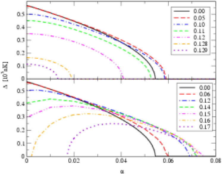
Figure 3.1: Dependence of the pairing gaps in the loff phase (upper panel) and the dfs phase (lower panel) on the density-asymmetry parameter for the values of the the pair momentum $P/k_{F}$ and deformation parameter $\delta\epsilon$ indicated in the legends. The Fermi momentum is $k_{F}=4.83\times 10^{4}$ cm^-1 and the scattering length is $a=-2160a_{B}$, so that $k_{F}|a|=0.55$. .

As expected, for vanishing asymmetries $\alpha\rightarrow 0$, the maximal gap is attained by the standard bcs ground state, which is indicated by the solid, black line in both panels. The symmetry-breaking states that are very different from it (e. g., a loff state with $P/k_{F}\gtrsim 0.1$ or a dfs state with $\alpha\gtrsim 0.1$) have notably smaller gaps.

The situation changes for increasing asymmetry. For example, the loff state with $P/k_{F}=0.05$ presents a larger gap than the asymmetric bcs state for $\alpha>0.03$, a density asymmetry for which also the dfs state with $\delta\epsilon=0.12$ has a gap larger than the bcs one. Finally, for $\alpha\geq\alpha_{\rm max}^{BCS}\approx 0.055$, the bcs state no longer presents a finite gap, while both the loff and dfs phases ‘survive’ up to higher asymmetries: $\alpha_{\rm max}^{LOFF}\approx 0.06$ (for $P/k_{F}=0.05-0.10$) and $\alpha_{\rm max}^{DFS}\approx 0.075$ (for $\delta\epsilon\approx 0.15$), respectively. It is also remarkable the presence of a ‘reentrance’ phenomenon in the dfs phase. For instance, consider the case $\delta\epsilon=0.17$ (blue, dotted curve). Such a large deformation shows a finite gap only for asymmetric systems, and a lower $\alpha_{\rm cr\,1}\approx 0.02$ and higher $\alpha_{\rm cr\,2}\approx 0.07$ critical asymmetries can be identified. As the quantity that determines the true ground state of the system is the free energy and not the size of the gap, we cannot tell from Fig. 3.1 what will be the structure of the ground state. However, before discussing this point in detail, we shall study some aspects of the excitation spectrum of the system.

3.4 Excitation spectra in the superfluid phases

To elucidate the dominance of the phases with broken space symmetries over the asymmetric bcs state, it is useful to consider the modifications implied by these phases to the quasiparticle spectra

$$E_{\bm{k}}^{\pm} =E_{A}\pm\sqrt{E_{S}^{2}+|\Delta|^{2}}\>.$$ (3.5)

These energies correspond to the poles of the propagators $G_{\uparrow\downarrow}$ of chapter 1. Physically, $E_{\bm{k}}^{+}$ is the excitation energy of the system when we move it from its ground state to a state with momentum $\bm{k}$ and (pseudo)spin $\uparrow$. For a non-interacting system for which the number of particles is not considered fixed, this can be accomplished in two ways:

• adding an $\uparrow$-particle with momentum $\bm{k}$, or

• removing a $\downarrow$-particle with momentum $-\bm{k}$.

Conversely, $-E_{\bm{k}}^{-}$ is the excitation energy when the system is forced to have $\bm{k}$ momentum and $\downarrow$ (pseudo)spin. Which is the process that ultimately will be required to actually perform these excitations is essentially determined by Pauli’s principle and the interactions in the medium. For example, a system composed only of $\uparrow$-particles ($\mu=\delta\mu=\mu_{\uparrow}/2$) at $T=0$, can only be excited to states $|\bm{k},\uparrow\rangle$ for momenta $k>k_{\uparrow}$, as for $k<k_{\uparrow}$ all states are already occupied and Pauli’s principle forbids a new $\uparrow$-particle to be added to the system below its Fermi momentum. The resulting system will have excitation energy $\hbar^{2}k^{2}/(2m)-\varepsilon_{F}\equiv E_{\bm{k}}^{+}$. For $k<k_{\uparrow}$, the reachable states are $|\bm{k},\downarrow\rangle$ with excitation energy $\varepsilon_{F}-\hbar^{2}k^{2}/(2m)\equiv-E_{\bm{k}}^{-}>0$, corresponding to the creation of a hole in the $\uparrow$-Fermi sea at $k$. Similar ideas hold for the interacting system, and for other values of the densities $\rho_{\uparrow}$ and $\rho_{\downarrow}$.

We call the reader’s attention to the minus sign in front of $E_{\bm{k}}^{-}$: this is due to the conventional way of assigning energies to hole excitations (see, e. g., [FW71], pp. 74–75 ): the more negative they are, the more excited state of the system we get. This is easily understood again in the pure $\uparrow$-system, where removing an $\uparrow$-particle from $k=k_{\uparrow}$ leaves the system in its ground state, and therefore the excitation energy is $\epsilon_{\mathrm{exc}}(k=k_{\uparrow})=0\equiv-E^{-}_{k_{\uparrow}}$. On the other hand, removing a particle at $k=0$ will leave the system in a highly excited state, corresponding to having promoted [in the ($N-1$)-particle system] the $\uparrow$-particle at $k=0$ to $k=k_{\uparrow}$; the corresponding excitation energy is $\epsilon_{\mathrm{exc}}(k=0)=\mu_{\uparrow}\equiv-E^{-}_{0}$. Therefore, the excitation energies of the system displayed in Fig. 3.2 are

• $E_{\bm{k}}^{\uparrow}:=E_{\bm{k}}^{+}=\sqrt{E_{S}^{2}+|\Delta|^{2}}+E_{A}$: excitation energy of the system with momentum $\bm{k}$ and (pseudo)spin $\uparrow$;

• $E_{\bm{k}}^{\downarrow}:=-E_{\bm{k}}^{-}=\sqrt{E_{S}^{2}+|\Delta|^{2}}-E_{A}$: excitation energy of the system with momentum $\bm{k}$ and (pseudo)spin $\downarrow$.

Let us turn now to the effects of the density asymmetry on the solution of the gap equation. We have seen in the previous chapter that, in the asymmetric bcs state, $E_{A}$ acts in the gap equation (1.23) to reduce the phase-space coherence between the quasiparticles that pair. In other words, $E_{A}\neq 0$ introduces a ‘forbidden region’ for the momentum integration in the gap equation [cf. Sect. 2.2, especially Eq. (2.2b) and Fig. 2.3]. The bcs limit is recovered for $E_{A}=0$, with equal occupations for both particles and perfectly matching $\uparrow$ and $\downarrow$ Fermi surfaces. This blocking effect is responsible for the reduction of the gap with increasing asymmetry and its disappearance above $\alpha=\alpha_{\rm max}^{BCS}\simeq 0.055$.

When the pairs move with a finite total momentum or the Fermi surfaces are deformed (and taking the symmetry-breaking axis as $z$ axis), the anti-symmetric part of the spectrum $E_{A}$ is modulated with the cosine of the polar angle [cf. Eqs. (3.3–3.4)]. In the plane-wave loff phase $E_{A}\propto\chi=\cos\theta$, while in the dfs phase, which is the object of our primary interest, we have

$$E_{S} =\epsilon_{\bm{k}}-\mu-\delta\mu\,\delta\epsilon\,\chi^{2}$$ (3.6a)

$$E_{A} =-\delta\mu+\mu\,\delta\epsilon\,\chi^{2}\;.$$ (3.6b)

This angular variation acts to restore the phase-space coherence for some values of $\chi$ at the cost of even lesser (than in the bcs phase) coherence for the other directions. That is, the width of the forbidden region in Fig. 2.3 now depends on the direction: it is reduced in the $xy$ plane and increased on the $z$ axis. This effect can be explicitely seen in Figure 3.2 which compares the quasiparticle excitation spectra in the bcs and dfs phases. Let us comment carefully this figure, as it contain much information. The first column shows the results for the usual symmetric bcs case; the second column has the results for the asymmetric bcs case with a moderate density asymmetry $\alpha=0.04$; finally, the third column contains the results for the dfs phase with the same asymmetry and the optimal deformation $\delta\epsilon=0.08$.  In all three columns, the top plot displays the excitation spectra $E_{\bm{k}}^{\uparrow}$ (black lines) and $E_{\bm{k}}^{\downarrow}$ (green lines) close to the Fermi momentum $k_{F}$. Solid lines correspond to the results along the symmetry-breaking $z$ axis, while the dashed lines in the last column stand for the spectra in the $xy$ plane in $k$-space. The figure in the top-left corner is equivalent to the lower panel in Fig. 1.2. The spectra for the asymmetric bcs case are shifted with respect to each other due to the fact that $E_{A}\neq 0$, cf. Eq. 3.5, but keep the rotational invariance. Finally, the plot for the dfs phase shows the effect of the $\chi$-dependence of the spectra: the solid curves along the symmetry-breaking axis (i. e., $\chi=1$ or $k_{\perp}=0$) have gone further apart, while the dashed lines corresponding to $\chi=0$ ($k_{z}=0$) have approached one another.

To better evaluate the rotational properties of each phase, the lower plots show $E_{\bm{k}}^{\uparrow\downarrow}$ as a function of $k_{z}/k_{F}$ and $k_{\perp}/k_{F}$. Keeping $k=\sqrt{k_{z}^{2}+k_{\perp}^{2}}$ constant amounts to moving along circles on the $k_{z}-k_{\perp}$ plane, therefore exploring the angular dependence of the functions. For the symmetric bcs case, both $\downarrow$ and $\uparrow$ excitation spectra are equal, have a minimum at $k=k_{F}$ and are rotationally symmetric. For an asymmetric system (second column) the $\uparrow$ and $\downarrow$ spectra are no longer equally deep, but $E_{\bm{k}}^{\downarrow}$ is deeper than $E_{\bm{k}}^{\uparrow}$. Therefore, the quasiparticles of one species, that are defined near the corresponding Fermi surface, are far (in phase space) from those of the other species. The third column shows the excitation spectra in the dfs phase, as given by Eqs. (3.3) and (3.5). Rotational symmetry is now broken, as the spectra along $k_{z}$ (solid lines) are different from the spectra perpendicular to $k_{z}$ (dashed lines).

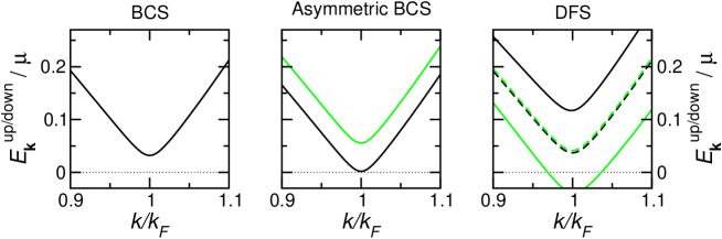
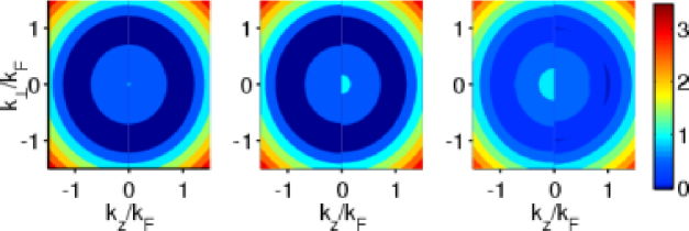
Figure 3.2: Dependence of the quasiparticle spectra $E_{\bm{k}}^{\uparrow}$ (black lines) and $E_{\bm{k}}^{\downarrow}$ (green) on the momentum for the symmetric bcs case (left); an asymmetric bcs case with $\alpha=0.04$ (center); and the optimal $\delta\epsilon=0.08$ dfs result for the same asymmetry (right). The $z$ axis is the symmetry-breaking axis of the dfs phase. In the top plots, the solid lines correspond to the spectra $E_{\bm{k}}^{\uparrow}$ (black) and $E_{\bm{k}}^{\downarrow}$ (green) along the $k_{z}$ axis. The dashed lines represent the results on the $xy$ plane ($k_{z}=0$) with the same color coding. The dotted line is at $E_{\bm{k}}=0$. In the lower plots, $E_{\bm{k}}^{\uparrow}$ is given only for $k_{z}>0$ and $E_{\bm{k}}^{\downarrow}$ for $k_{z}<0$.

A most remarkable feature in the dfs is that the energy separation between the quasiparticle spectra along the symmetry-breaking axis is considerably larger than in the asymmetric bcs state; in the orthogonal directions the opposite holds. Compared to the asymmetric bcs state, the phase-space overlap between pairs is accordingly decreased in the first region and increased in the second. The net result, displayed in Figure 3.3, is the increase in the value of the critical asymmetry $\alpha_{\rm max}$ at which superfluidity vanishes. As noted above, at large asymmetries the dfs phase exhibits the re-entrance effect: pairing exists only for the deformed state between the lower and upper critical deformations ($\alpha_{\rm cr\,1}\neq 0$). We note that to obtain this effect the recalculation of the chemical potentials through the normalization condition on the densities is essential, as it affects dramatically the value of $\delta\mu$, that enters $E_{A}$.

Figure 3.3: Dependence of the critical asymmetry of the transition from the superfluid to the normal state on the pair momentum in the loff phase (solid line) and the deformation parameter in the dfs phase (dashed and dot-dashed lines).

Notice also that in the asymmetric systems, the $\downarrow$ spectrum is gapless in a region of momentum space defined by

$$E_{\bm{k}}^{\downarrow}\equiv E^{\downarrow}(k_{z},k_{\perp})\leq 0\;.$$ (3.7)

The possibility of exciting the system without energy cost has important consequences for the dynamical properties of the paired states, such as the transport and the collective modes, and leads to a number of peculiarities in their thermodynamics [Sar63, SAL97, SL00, LW03, SH03, HS03, WY03]. That is, the macro-physical manifestations of the loff and dfs phases such as the response to density perturbations or electromagnetic probes and the thermodynamic functions (heat capacity, etc) will differ from the ordinary bcs  phase due to the nodes and anisotropy of their spectra. We will show in Sect. 3.6 how such an anisotropy can be used to discriminate phases with broken space symmetries in time-of-flight experiments. We remark finally that the phases with broken space symmetries (loff and dfs) present a larger number of excitation modes because of the breaking of global space symmetries; these additional modes are usually called Goldstone modes [Gol61, PS95].

3.5 Determining the ground state

3.5.1 Calculation of the free energy

The phase that must be identified as the equilibrium state at a given density asymmetry and temperature is the one that has the lowest free energy. We have calculated the free energy for each candidate phase (bcs, loff, dfs) in the following way.

We have defined the free energy as usual by

$${\cal F}=E_{\rm kin}+E_{\rm pot}-T{\cal S},$$ (3.8)

where the first two terms comprise the internal energy which is the statistical average of the Hamiltonian (1.4), $T$ is the temperature and ${\cal S}$ the entropy, given for a gas of fermions by the well-known expression [FW71],

$${\cal S} =-k_{B}\int\frac{\mathrm{d}^{3}k}{(2\pi)^{3}}\,\sum_{s=\uparrow,\downarrow}\big{\{}\left(1-n_{s}(\bm{k})\right)\ln\left[1-n_{s}(\bm{k})\right]+n_{s}(\bm{k})\ln\left[n_{s}(\bm{k})\right]\big{\}}\>.$$

For a contact potential of strenght $g$ , the potential energy is easily evaluated, and we have

$$E_{\rm kin}+E_{\rm pot} =\int\frac{\mathrm{d}^{3}k}{(2\pi)^{3}}\,\epsilon_{\bm{k}}\left[n_{\uparrow}(\bm{k})+n_{\downarrow}(\bm{k})\right]-\frac{\Delta^{2}}{g}\>,$$ (3.9)

$$n_{s}(\bm{k}) =u^{2}(\bm{k})f(E_{\bm{k}}^{s})+v^{2}(\bm{k})\left(1-f(E_{\bm{k}}^{-s})\right)\>.$$ (3.10)

The free energy of the undeformed normal state follows by setting in the above expressions $\Delta=0=\delta\epsilon$, while that of the bcs phase is given by $\Delta\neq 0=\delta\epsilon$, and so on for the loff and dfs phases (see Table 3.1).

Because of the contact form that we use for the interaction, the gap equation and the superfluid kinetic energy need a regularization. There are several ways to regularize the gap equation. We can write them formally together in the form [cf. Eq. (1.23)]

$$1=\frac{g}{2}\int_{0}^{\Lambda}\!\!\frac{\mathrm{d}kk^{2}}{(2\pi)^{2}}\int_{-1}^{1}\!\!\mathrm{d}\chi\left(\frac{f_{F}(E_{\bm{k}}^{+})-f_{F}(E_{\bm{k}}^{-})}{\sqrt{E_{S}^{2}+\Delta^{2}}}+\frac{\gamma}{\epsilon_{\bm{k}}}\right),$$ (3.11)

where $f_{F}$ is the usual Fermi distribution function. The case $\gamma=1$ and $\Lambda\to\infty$ corresponds to the common practice of regularization [SHSH96], which combines the gap equation with the T-matrix equation in free space, and is the one we have used in chapter 2. Choosing $\gamma=0$ and a finite $\Lambda$ corresponds to the cut-off regularization of the original gap equation. The appropriate cutt-off in this second scheme is found by requiring both schemes to give the same value for the gap. Then, this $\Lambda$ is used to evaluate the kinetic energy contribution to the free energy. We note once more that Eq. (3.11) must be solved together with the normalization constraints on the densities

$$\rho_{s} =\int\frac{\mathrm{d}^{3}k}{(2\pi)^{3}}\,n_{s}(\bm{k})\qquad(s=\uparrow,\downarrow)\>.$$ (3.12)

3.5.2 Analytical estimation of the optimal deformation

Before comenting the numerical results, it is instructive to perform an analytical estimation of the deformation $\delta\epsilon$ of the Fermi surfaces that one expects will maximize the pairing energy.

The physical idea behind the deformation of the Fermi surfaces of the pairing species is to approach them in some regions of momentum space, so that the quasiparticles’ phase space has a sizeable overlap. If this deformation had no kinetic energy cost, we can imagine that the optimal deformation would be the one that effectively makes the two Fermi surfaces be as close to each other as possible, given the constraint of the conservation of the different densities. Thus, we will calculate which deformation $\delta\epsilon$ brings the outermost part of the Fermi surface of the least populated species and the innermost part of the Fermi surface of the majority to touch. The optimal deformation is somewhat different that the one predicted by this estimation because of the investment in kinetic energy that this deformation requires. In any case, we can get a good estimate of the optimal $\delta\epsilon$ in this simple way.

We assume for simplicity $T=0$ and start from Eq. (3.4). Here, we must understand $\mu_{s}=\hbar^{2}\widetilde{k}_{s}^{2}/(2m)$, where $\widetilde{k}_{s}$ is such that the density of $s$-particles is conserved. For the case of $\uparrow$-particles:

$$\rho_{\uparrow} =\int\frac{\mathrm{d}^{3}k}{(2\pi)^{3}}\,\Theta\left[\widetilde{k}_{\uparrow}^{2}\left(1+\delta\epsilon\cos^{2}\theta\right)-k^{2}\right]$$

$$=\frac{1}{(2\pi)^{2}}\frac{\widetilde{k}_{\uparrow}^{3}}{24}\left[2\sqrt{1+\delta\epsilon}(5+2\delta\epsilon)+6\frac{\operatorname{arcsh}{\sqrt{\delta\epsilon}}}{\sqrt{\delta\epsilon}}\right]$$ (3.13)

The expression for $\rho_{\downarrow}(\widetilde{k}_{\downarrow})$ is analogous with $\delta\epsilon\rightarrow-\delta\epsilon$. As the ‘true’ Fermi momentum of $\uparrow$-particles is defined by $\rho_{\uparrow}=\rho(1+\alpha)/2=k_{\uparrow}^{3}/(6\pi^{2})$, we have

$$\frac{k_{\uparrow}^{3}}{k_{\downarrow}^{3}} \equiv\frac{1+\alpha}{1-\alpha}\>,$$

$$=\frac{\widetilde{k}_{\uparrow}^{3}}{\widetilde{k}_{\downarrow}^{3}}\frac{2\sqrt{1+\delta\epsilon}(5+2\delta\epsilon)+6\frac{\operatorname{arcsh}{\sqrt{\delta\epsilon}}}{\sqrt{\delta\epsilon}}}{2\sqrt{1-\delta\epsilon}(5-2\delta\epsilon)+6\frac{\operatorname{arcsh}{\sqrt{\delta\epsilon}}}{\sqrt{\delta\epsilon}}}\approx\frac{\widetilde{k}_{\uparrow}^{3}}{\widetilde{k}_{\downarrow}^{3}}\left(1+\frac{9}{8}\delta\epsilon\right)$$

where the last result follows for $\delta\epsilon\ll 1$. In the plane perpendicular to the symmetry-breaking axis ($\cos\theta=0$), each momentum distribution vanishes at the corresponding $\widetilde{k}_{s}$. Therefore, we will have an exact matching of the two Fermi surfaces in this plane for $\widetilde{k}_{\uparrow}=\widetilde{k}_{\downarrow}$. Then, for a given $\alpha$ we can obtain our estimation for the optimal deformation from the last equation:

$$\delta\epsilon_{\rm opt}=\frac{16}{9}\frac{\alpha}{1-\alpha}\>.$$ (3.14)

Substitution of this value into (3.13) gives the new value for $\widetilde{k}_{\uparrow}$, and therefore the new chemical potential $\mu_{\uparrow}$, and analogously for $\mu_{\downarrow}$. For $\alpha\ll 1$ we expect a deformation $\delta\epsilon_{\rm opt}\approx(16/9)\,\alpha\approx 2\alpha$. We will see that this approximation agrees reasonably well with the numerical calculations below, even though the overlap is not perfect in the numerical solution because in this analysis we have disregarded the investment in kinetic energy.

3.5.3 Numerical results

We plot in Fig. 3.4 the difference $\Delta{\cal F}={\cal F}_{S}-{\cal F}_{N}$ between the free energy ${\cal F}_{S}$ of the superfluid phase (either bcs, loff or dfs) and the free energy ${\cal F}_{N}$ of the normal state ($\Delta,\delta\epsilon,P=0$). The bcs result is plotted in both panels as the black solid line, while the results for the loff phase are summarized in the top panel for various values of $P/k_{F}$. The lower panel contains the corresponding results for the dfs phase for a variety of $\delta\epsilon$’s. First of all, a simple comparison of this figure with 3.1 shows that $\Delta{\cal F}$ closely follows the behavior of $-\Delta^{2}$. However, the contribution from the kinetic energy to ${\cal F}$ introduces some important differences as, for example, the delay in the dfs being preferable to the normal phase, e. g. for $\delta\epsilon=0.17$ from $\alpha\approx 0.018$ (where a non-vanishing gap appears) to $\alpha\approx 0.025$ (where $\Delta{\cal F}<0$).

The loff phase is preferred to the normal and the bcs phases in a narrow window of asymmetries $0.04\leq\alpha\leq 0.057$ and for a total momentum of the pairs $P/k_{F}\sim 0.05$, as shown by the red dashed line lying below the solid one. This is consistent with the results obtained in the scheme where the density asymmetry is described by fixing the difference in chemical potentials of the pairing species $\delta\mu$. In this approach, the critical value for the bcs phase is $\delta\mu_{c}^{BCS}=0.707\Delta(0)$, while for the loff phase $\delta\mu_{c}^{LOFF}=0.755\Delta(0)$, where $\Delta(0)\equiv\Delta(\delta\mu=0)$ [LO64, FF64]. Note that while there is a non-trivial solution to the gap equation for $P/k_{F}\geq 0.1$ the gain in pairing energy is less than the investment required in kinetic energy due to the motion of the condensate, and the net free energy of the loff phase is greater than that of the asymmetric bcs phase for these momenta. However the pairing energy of the loff phase could be improved by choosing a more complex form of the order parameter, e. g. by keeping a larger number of terms in its expansion in the Fourier series.

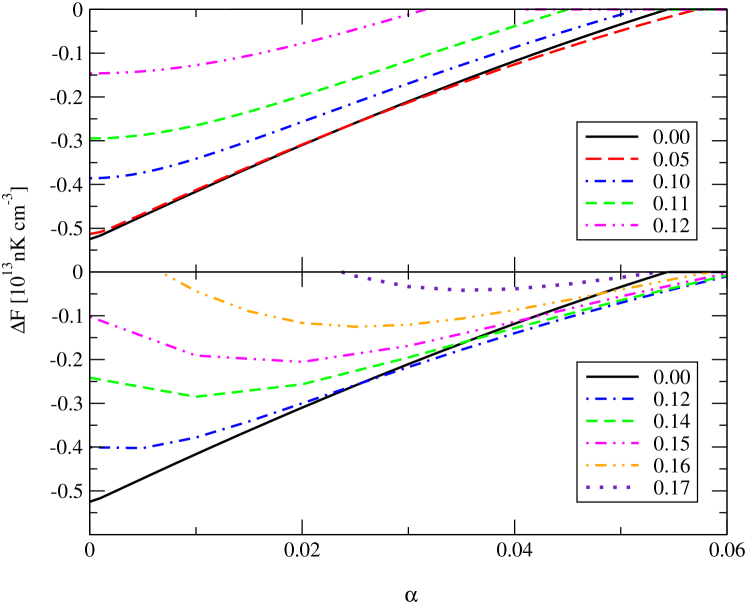
Figure 3.4: Difference of the free-energy density of the plane-wave loff (upper panel) and dfs (lower panel) phases with respect to the normal phase, as a function of the asymmetry parameter $\alpha$, for the values of the pair momentum $P/k_{F}$ and the deformation parameter $\delta\epsilon$ indicated in the legends.

.

The dfs phase is the ground state of the system in a wider range of asymmetries $0.03\leq\alpha\lesssim 0.06$ for the deformation parameter in the range $0.12\leq\delta\epsilon\leq 0.14$. For even larger deformations the gain in pairing energy does not compensate the investment in kinetic energy due to the ellipsoidal stretching of the Fermi surfaces: the curve for $\delta\epsilon=0.17$ lies always above the bcs one. We note finally that the free energy is also affected by the re-entrance effect (i. e., restoration of pairing correlations as the asymmetry is increased), but in fact we do not find that this effect is responsible for the ground state at these weak couplings: the free energy for the case $\delta\epsilon=0.16$ lies in our calculations always above those for $\delta\epsilon\leq 0.15$, which do not present re-entrance, in contrast to what happens in more strongly-coupled systems such as neutron-proton pairing at saturation density [MS02] or ‘two color superconductivity’ between up and down quarks in dense hadronic matter [MS03a].

To summarize, the coherence is restored and the strength of pair-correlations is increased in the loff phase due to the finite momentum of the Cooper pairs. In the dfs phase, the same is achieved by stretching the spherical Fermi surfaces into ellipsoids. The fundamental difference between these phases is that translational symmetry remains intact for the dfs phase, as it breaks only the rotational symmetry, while the loff phase breaks both symmetries. Quantitatively, the maximal value of the gap and the absolute value of the ground-state free energy are larger in the dfs phase than in the loff phase for asymmetries $\alpha\gtrsim 0.04$. For these asymmetries both phases are favorable over the homogeneous bcs phase. However, one should keep in mind that the loff phase admits a variety of lattice forms, and the plane-wave structure might not be the most favored one [ABR01, Sed01, BR02, CN04].

3.6 Detecting the dfs phase in experiments

Experimental evidence for the phases with broken space symmetries can be obtained from the studies of their momentum distributions which, unlike in the homogeneous phase, must be anisotropic in space. Indeed, from Eqs. (3.5), (3.6) and (3.10), we see that, for $\delta\epsilon\neq 0$, the probability of a $s$-particle having momentum $\bm{k}$, $n_{s}(\bm{k})$, will depend on $k_{z}^{2}$ and $k_{\perp}^{2}$ separately or, equivalently, on $k=|\bm{k}|$ and $\chi=\cos\theta=k_{z}/k$, and not only on the scalar combination $k^{2}=k_{z}^{2}+k_{\perp}^{2}$.

In this case, it is useful to analyze the angular anisotropy in momentum space of the occupation numbers, that we define as

$$\delta n_{s}(k)=|n_{s}(k;\chi=1)-n_{s}(k;\chi=0)|\;.$$ (3.15)

This quantity vanishes for rotationally-invariant systems, and can be taken as a measure of the degree of symmetry breaking of a given phase. For example, $\delta n_{s}(k)\equiv 0\leavevmode\nobreak\ (\forall k)$ for the symmetric and asymmetric bcs solutions to the gap equation. For the dfs phase, the momentum distributions for each species depend on $\chi$, and we expect that $\delta n_{s}$ will not vanish but present a maximum around the corresponding Fermi momentum $k_{s}$.

We show in Fig. 3.5 the momentum distributions for the same system as in Fig. 3.1: $k_{F}=4.83\times 10^{4}$ cm^-1 (indicated by the vertical line) and $a=-2160a_{B}$. For clarity, we present only the data around $k_{F}$, where all the interesting physics happens. There are four sets of curves corresponding to the symmetric bcs phase (thin solid line), asymmetric bcs with $\alpha=0.04$ (dashed lines) and dfs with the same asymmetry and $\delta\epsilon=0.08$ for $\chi=0$ (dash-dotted lines) and $\chi=1$ (dotted lines), respectively. For the $\alpha\neq 0$ cases, blue lines correspond to $n_{\uparrow}(\bm{k})$ while red lines are for $n_{\downarrow}(\bm{k})$. Finally, the thick, bell-shaped curves correspond to $\delta n_{s}(k)$ with the same color coding.

The Fermi surfaces of the symmetric bcs phase are spread around $k_{F}$ over a width of the order of $k_{F}\,\Delta/\varepsilon_{F}$. One should notice that some broadening of the surface is also due to the finite temperature assumed in the calculations. The asymmetric bcs distributions (dashed lines) show a similar shape, but with the characteristic decays centered around the corresponding Fermi momenta $k_{\downarrow}\approx 4.75\times 10^{4}$ cm^-1, $k_{\uparrow}\approx 4.91\times 10^{4}$ cm^-1. At the low temperature studied, the momentum distributions still fall off very fast, and the two Fermi surfaces are separated $\sim 0.16\times 10^{4}$ cm^-1, thus triggering the Pauli blocking effect commented in Sect. 2.2.

The situation changes when looking at the dfs results which show a clear dependence on $\chi$. First of all, we notice that the dfs curves for $\chi=0$ (dash-dotted lines) are almost indistinguishable, while the results for $\chi=1$ (dotted lines) are further apart. This means that the (ellipsoidal) Fermi surfaces of $\uparrow$ and $\downarrow$ particles have approached each other in the $xy$ plane in momentum space, while they have gone apart along the $z$ direction (see Fig. 3.5). Note also that the range of occupations covered by the dfs curves includes the asymmetric bcs results. One could have expected the asymmetric bcs results to coincide with the dfs ones for $\chi=0$, as in both cases the symmetry-breaking term $\delta\epsilon\,\chi^{2}$ vanishes [see Eq. (3.6)]. However, the fully self-consistent solution of the gap equation together with the number equations involves a re-calculation of the chemical potentials for the dfs case, resulting in new effective Fermi momenta $\widetilde{k}_{s}$ (see Sect. 3.5.2) which become very similar to each other and to $k_{F}$. That is the reason why the dfs results at $\chi=0$ are so close to each other, and relatively far from the asymmetric bcs ones. In addition, we obtain a larger gap (cf. Fig 3.1), that translates into slightly softer decays of the dfs momentum distributions as compared with those for the asymmetric bcs case.

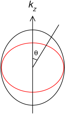
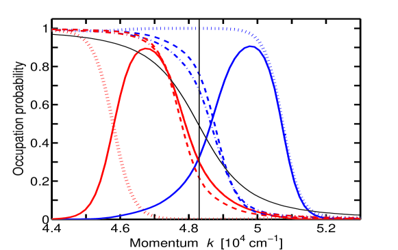
Figure 3.5: Dependence of the occupation probabilities of two hyperfine states on the momentum. The Fermi momentum $k_{F}=4.83\times 10^{4}$ cm^-1 is indicated by the vertical line. The labeling of the lines is as follows: $\alpha=0=\delta\epsilon$ (black, solid line), $\alpha=0.04$ and $\delta\epsilon=0$ (dashed lines); $\alpha=0.04$, $\delta\epsilon=0.08$, $\chi=0$ (dash-dotted) and $\chi=1$ (dotted). The blue lines are for $\uparrow$ particles (major population, see left), while the red ones are for $\downarrow$ particles (minority). The bell-shaped curves show the anisotropy as defined by Eq. (3.15) for $\alpha=0.04$, $\delta\epsilon=0.08$.

The anisotropy in the dfs occupation probabilities along the directions parallel and orthogonal to the symmetry-breaking axis reaches a maximum of more than 90% for both species centered at different momenta: for $\delta n_{\downarrow}$, around $\widetilde{k}_{\downarrow}\sqrt{1-\delta\epsilon}\approx 4.63\times 10^{4}$ cm^-1 [momentum for which $\delta n_{\downarrow}(\chi=0)\approx 1$ and $\delta n_{\downarrow}(\chi=1)\approx 0$]; for $\delta n_{\uparrow}$, at $\widetilde{k}_{\uparrow}\sqrt{1+\delta\epsilon}\approx 5.07\times 10^{4}$ cm^-1 [where $\delta n_{\uparrow}(\chi=0)\approx 0$ and $\delta n_{\uparrow}(\chi=1)\approx 1$].

In practice, this means that one expects to find more $\uparrow$ particles with momenta $k>k_{F}$ in the $z$ direction ($\chi=1$) than in the radial direction ($\chi=0$), while the opposite holds for the $\downarrow$ particles. Thus, a direct way to detect the dfs phase is a measurement of this crossed anisotropy in the momentum distributions of the trapped atoms. Such a measurement can be realized by the time-of-flight technique [JILA95, MIT95, Rice99]. This method uses the fact that after switching off the trap, the atoms fly out freely and an image of their spatial distribution taken after some time of flight provides information on their momentum distribution when confined inside the trap. Assuming that the system was in the deformed superfluid state one would detect a number of particles of type $\uparrow$ (majority) in the direction of symmetry breaking by about 90% larger than in any orthogonal direction, and viceversa for the $\downarrow$ particles (minority). Therefore, the presence of this crossed anisotropy in the detected momentum distributions would be an evidence for a ‘deformed superfluid state’ being the ground state of the system, as deformation alone (i. e., without pairing) would not lower the energy so as to produce a deformed non-superfluid ground state. Note that this argument is equally valid for a homogeneous system or for an atomic sample in a spherical trap, where no privileged direction is introduced by the trapping potential. For a non-spherical trap, the normal-state momentum distributions of both species are expected to be deformed in the same way. Therefore, the detection of a crossed anisotropy in the momentum distributions as discussed above would also be a strong case for the dfs phase being the ground state of the system. However, a more specific calculation (e. g., in local density approximation in the trap) would be necessary to quantify this effect and study the influence of the trap anisotropy on the momentum distributions in the different phases.

We remark finally that the direction of spontaneous symmetry breaking (in $k$-space and, therefore, also in real space) is chosen by the system randomly and needs to be located in an experiment to obtain maximum anisotropy. Also, a clear distinction between the dfs and the loff phases can be achieved in the time-of-flight experiments, since the latter predicts periodic momentum distributions.

3.7 Summary

In this chapter we have studied the possibility to generalize the bcs ground state by letting the Cooper pairs carry a finite center-of-mass momentum (the so-called loff phase) or by deforming the Fermi surfaces of the pairing species (dfs phase). For the density-symmetric case ($\alpha=0$), the bcs pair wave-function is the best among these three options, i. e., it gives the lowest free energy for the system. However, for systems with different populations of the two species ($\alpha\neq 0$), this is only true for very small asymmetries ($\alpha<0.03=3\%$). For larger asymmetries, the loff and/or dfs phases become preferable. Our quantitative analysis has shown that, at weak-coupling, the dfs phase is prefered to the normal, bcs and plane-wave loff phases (though more general forms for the loff phase are possible and might lower further the free energy). We note that similar conclusions have been earlier reported for strongly-coupled systems such as neutron-proton pairing in asymmetric nuclear matter in the ${}^{3}S_{1}-^{3}D_{1}$ channel [MS02, MS03b] and pairing of up and down quarks of two colors in dense hadronic matter [MS03a]. Therefore, we expect a similar behavior for more strongly-coupled atomic systems, such as those produced by means of magnetic Feshbach resonances to study the BCS-BEC crossover [JILA03a, MIT03, Rice03, Inns04, ENS04a, Duke05].

We have finally shown how the dfs phase can be detected in an ultracold gas of fermionic atoms in a spherical trap by studying the momentum distribution of the released atoms in a time-of-flight experiment.

Chapter 4 Pairing in boson-fermion mixtures

His house was perfect whether you liked food, or sleep, or work, or story-telling, or singing, or just sitting and thinking best, or a pleasant mixture of them all.

J. R. R. Tolkien, The Hobbit

4.1 Introduction

Mixtures of quantum fluids of different statistics have been an interesting field of research for a long time, specially in the context of helium systems, where the fraction of ³He (fermion) in a homogeneous ⁴He (boson) medium is limited to $x_{3\rm max}\approx 6.5\%$. For $x_{3}>x_{3\rm max}$ the system becomes unstable and separates into a mixed phase with a ³He concentration $x_{3\rm max}$ and another phase with pure ³He atoms.

Since the first achievement of Bose-Einstein condensation, the purpose of building an analogous ultracold Fermi system had to overcome the cooling limitations established by Pauli’s exclusion principle, that forbids $s$-wave collisions between indistinguishable fermions. This problem can be solved in a boson-fermion mixture, as the bosonic component can be ‘easily’ cooled and, by thermal contact, drives the fermionic component down to ultralow temperatures, as was first achieved at Rice University when a gas of ⁶Li was driven to the degenerate regime by sympathetically cooling it with ⁷Li [Rice01].

After this experiment, many others have shown the feasibility of studying interesting quantum phenomena in ultracold fermionic systems. For example, the lens group used ⁸⁷Rb-⁴⁰K mixtures with varying numbers of atoms of both species to study the collapse predicted by mean-field theory [M l98, RF02] and extracted a value for the interspecies scattering length $a\left(\mbox{${}^{87}$Rb-${}^{40}$K}\right)=-22$ nm [LENS02].

In this chapter, we address the problem of determining the fermion-fermion interaction inside a dilute mixture of bosons and fermions. This problem is important as medium effects can have dramatic consequences on the behavior of the system. A classical example is that of superconductivity in metals, where the phonon-mediated interactions between electrons give rise to an attraction between the latter, thus triggering the Cooper instability of the system and resulting in the superfluid behavior of the electronic component [Sch88]. First, we will review the three-dimensional situation, already studied by Viverit et al.[VPS00, BHS00]. Then, we will study the two-dimensional case, where the reduction in the dimensionality of the phase space makes one expect that correlations will play a more important role as compared to the 3D situation. Indeed, today’s available capabilities to manipulate trapped, atomic gases allow for the production of effectively one- and two-dimensional systems by the deformation of the traps or, more efficiently, by shining on it an array of standing light-waves that produce a kind of periodic potential known as optical lattice (see, [GV99, NIST02] and references therein). We will end up applying the developed model to the cases of ⁸⁷Rb-⁴⁰K and ⁷Li-⁶Li mixtures under current experimental investigation.

4.2 Three-dimensional mixtures

Let us start by considering the fermion-fermion ($FF$) interaction in three-dimensional space for a one-component fermionic system in the presence of bosons. At the ultralow temperatures of interest $T\lesssim 10\mu$K and dilute conditions of present experiments, only $s$-wave collisions are relevant (unless they are absent). As for a system of indistinguishable fermions $s$-wave interactions are forbidden by Pauli’s principle, we will be left only with the boson-fermion ($BF$) and boson-boson ($BB$) interactions, while the direct $FF$ one can be neglected. For a dilute and ultracold system, these collisions can be modeled in three dimensions by a contact interaction or, equivalently, by momentum-independent T-matrices,

$$\textsf{T}_{\rm BF} =\frac{4\pi\hbar^{2}}{m_{BF}}a_{BF}$$

$$\textsf{T}_{\rm BB} =\frac{4\pi\hbar^{2}}{m_{B}}a_{BB}\>,$$

where $m_{B}$ ($m_{F}$) is the mass of a boson (fermion) and $m_{BF}=m_{B}m_{F}/(m_{B}+m_{F})$ is the reduced mass in a boson-fermion collision.

The boson-induced fermion-fermion interaction can be represented by the diagram in Fig. 2.2(b), where now the bubble corresponds to a density fluctuation in the bosonic medium. Analogously, we can use a formula similar to Eq. (2.6):

$$\left\langle\bm{k^{\prime}}|\Gamma_{F}|\bm{k}\right\rangle=\Pi_{B}^{\rm RPA}\left(|\bm{k^{\prime}}-\bm{k}|\right)\textsf{T}_{\rm BF}^{2}\>.$$ (4.1)

Here $\Pi_{B}^{\rm RPA}$ stands for the density-density response function of the bosonic component in the random phase approximation (RPA). Already from its diagrammatic representation [Fig. 4.2(b)], one can see that it is possible to evaluate $\Pi_{B}^{\rm RPA}$ as a series once $\textsf{T}_{\rm BB}$ and the bosonic Lindhard function $\Pi_{B}$ are known. For in- and out-going fermions on their Fermi surface there will be no net energy transfer through the bosonic medium [Fig. 4.2(a)], and one can take the static limit $\omega=0$ for the bosonic response function [NP90, FW71],

$$\Pi_{B}(q;\omega=0)=-\frac{4m_{B}\rho_{B}}{\hbar^{2}q^{2}}\>.$$

Altogether, we get

$$\Pi_{B}^{\rm RPA}(q)=\frac{\Pi_{B}(q)}{1-\textsf{T}_{\rm BB}\Pi_{B}(q)}\>.$$ (4.2)

Note that, due to the low density of the systems we are interested in, we are neglecting any fermionic influence on the bosonic component.

As in Sect. 2.4, we must now project this polarization-induced interaction onto its $p$-wave contribution with the corresponding Legendre polynomial. Again, for a weakly-interacting system it is sufficient to consider only the case where both in- and out-going fermions are on their Fermi surface:

$$\Gamma_{F}^{(L=1)}(k_{F},k_{F})={\textsf{T}_{\rm BF}^{2}}\int_{-1}^{+1}\frac{dz}{2}z\Pi^{\rm RPA}_{B}(\sqrt{2(1-z)}k_{F})=-\frac{\textsf{T}_{\rm BF}^{2}}{\textsf{T}_{\rm BB}}h_{\rm 3D}\!\left(x\right)\>,$$ (4.3)

with $x=\hbar^{2}k_{F}^{2}/(m_{B}\rho_{B}\textsf{T}_{\rm BB})=2(\varepsilon_{F}/\mu_{B})(m_{F}/m_{B})$ [for a dilute, homogeneous bosonic system, $\mu_{B}=\textsf{T}_{\rm BB}\rho_{B}$], and the function

$$h_{\rm 3D}(x):=\frac{2}{x}\left[\left(\frac{1}{x}+\frac{1}{2}\right)\ln\left(1+x\right)-1\right]\>,$$

which is plotted in Fig. 4.1.

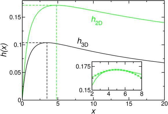
Figure 4.1: The functions governing the boson-induced fermion-fermion interaction in three (lower curve) and two (upper curve) dimensions. The dashed lines indicate the position and value of the corresponding maxima. The inset shows $h_{\rm 2D}$ together with the quadratic approximation around its maximum (thin line with crosses).

This function presents a broad maximum at ($x^{3D}_{\rm opt}\approx 3.48,\leavevmode\nobreak\ h^{3D}_{\rm opt}\approx 0.10$). This means that the induced interaction is optimized for a particular boson/fermion ratio given by

$$\frac{\rho_{F}^{2/3}}{\rho_{B}}\approx 2.88\,a_{BB}\>,$$

or, in terms of energies,

$$\frac{\varepsilon_{F}}{\mu_{B}}\approx 1.74\,\frac{m_{B}}{m_{F}}\>.$$

For example, for the case of mixtures of ⁸⁷Rb (boson) and ⁴⁰K (fermion) ($a_{BB}=5.2$ nm [vKKHV02]), this relationship gives $\rho_{F}=1.8\times 10^{14}$ cm^-3 for the case $\rho_{B}=10^{16}$ cm^-3, or $\varepsilon_{F}=138$ nK for $\mu_{B}=36$ nK. Estimating the resulting $p$-wave gap for the optimal boson concentration by means of Eq. (2.9), we get for these densities $\Delta_{1}/\mu_{F}\sim 10^{-7}$, which corresponds to an unattainable critical temperature.

4.3 Two-dimensional mixtures

Pairing in two dimensions has the peculiar feature that, for an attractive $s$-wave interaction between two different fermionic species, a two-particle bound state (of binding energy $E_{b}$) is always present, no matter how weak the attraction is. Therefore the system enters the strong-coupling regime even at low densities [SRVR89, RDS89, RDS90, PBS03], forming a Bose condensate of fermion pairs characterized by

$$\mu_{F} \rightarrow\varepsilon_{F}-E_{b}/2\>,$$

$$\Delta_{s} \rightarrow\sqrt{2E_{b}e_{F}}\>,$$

where $\Delta_{s}$ is the $s$-wave pairing gap in 2D. This is in clear contrast to the three-dimensional case for two reasons: (a) in 3D, a two-body (i. e., in a vacuum) bound state requires a minimum strength of the (attractive) potential, and (b) a bound state in the many-body system is only very weakly bound in the low density limit (the gap vanishes exponentially with $k_{F}\rightarrow 0$).

In three dimensions a small excess of one type of fermions implied an important reduction of the gap, and eventually its disappearance even for very small asymmetries (see Sect. 2.2). The situation in the strong-coupling regime is very different. Here, the system will form all possible pairs, while the remaining particles just stay in their original unpaired states, in close analogy with the behavior of nuclear matter at densities low enough to allow for the formation of deuterons (deeply bound neutron-proton pairs) [LNS⁺01].

We therefore exclude in the following this ‘trivial’ case, and focus on treating a system of identical (spin-polarized) fermions. The first possibility of pairing concerns the $p$-wave pairing gap, $\Delta_{1}\equiv\Delta_{L=1}(k_{F})$, which in the low-density limit is given by the weak-coupling result [RDS90]

$$\frac{\Delta_{1}}{\mu_{F}}=c_{1}\exp\!\left[-\frac{2\pi\hbar^{2}}{m_{F}\textsf{T}_{F}}\right]\>,$$ (4.4)

where $c_{1}$ is a constant of order unity and

$$\textsf{T}_{F} =\textsf{T}_{F}^{(L=1)}(k_{F},k_{F};2\mu_{F})=\int_{0}^{\pi}\frac{d\phi}{\pi}\cos{\phi}\left\langle\bm{k^{\prime}}|\textsf{T}(2\mu_{F})|\bm{k}\right\rangle\;,$$ (4.5)

$$|\bm{k}|=|\bm{k^{\prime}}|=k_{F}\>,\qquad\cos{\phi}=\bm{\widehat{k}}^{\prime}\cdot\bm{\widehat{k}}\;,$$

is the relevant T-matrix element of the interaction, computed at collision energy $2\mu_{F}$. Note that the two-dimensionality of the system is reflected already in the integration to be performed over the angle $\phi$, in contrast to the 3D case, where we could integrate directly over $z=\cos(\phi)$ [cf. Eq. (4.3)].

Let us consider a homogeneous mixture of bosons and fermions, and disregard for the moment the possibility of a direct $p$-wave interaction between the latter. The most important contribution to the $FF$ interaction is then given by the density fluctuations in the boson condensate sketched in Fig. 4.2.

Figure 4.2: (a) Polarization interaction $\Gamma$ between two fermions (dashed lines) mediated by the presence of bosons (solid lines). The labels indicate the momentum and energy of each line. For condensate bosons and fermions on the Fermi surface, $\bm{h}=\bm{0},\omega=0$. (b) Diagrams contributing to the boson bubble in RPA; the last one is an example of a backwardgoing diagram, negligible when $\mu_{B}\rightarrow 0$. Here, thick solid lines are full propagators, thin solid lines are free propagators, and wiggles represent interactions.

4.3.1 Constant T-matrices

As a first approach to the problem, we take $\textsf{T}_{\rm BF}$ and $\textsf{T}_{\rm BB}$ to be constants as in three dimensions. Thus, the treatment is completely analogous to that of Sect. 4.2, and we just have to evaluate the integral in Eq. (4.5). We obtain

$$\Gamma^{(L=1)}_{k_{F}k_{F}} ={\textsf{T}_{\rm BF}^{2}}\int_{0}^{\pi}\frac{d\phi}{\pi}\cos{\phi}\;\Pi^{*}_{B}(\sqrt{2(1-\cos{\phi})}k_{F})=-\frac{\textsf{T}_{\rm BF}^{2}}{\textsf{T}_{\rm BB}}h_{\rm 2D}\left(x\right)\>,$$ (4.6)

where $x=\hbar^{2}k_{F}^{2}/(m_{B}\textsf{T}_{\rm BB}\rho_{B})$ as before, and

$$h_{\rm 2D}(x):=\frac{2+x}{x\sqrt{1+x}}-\frac{2}{x}\>.$$ (4.7)

This function has a maximum located at ($x^{2D}_{\rm opt}=2/(\sqrt{2}-1)\approx 4.828,\leavevmode\nobreak\ h^{2D}_{\rm opt}=3-2\sqrt{2}\approx 0.172$), and can in its vicinity be approximated by a parabola, as shown in the inset of Fig. 4.1. This translates into a sharp Gaussian peak for the gap function, according to the weak-coupling result (4.4).

Note that, even though $x^{3D}_{\rm opt}$ and $x^{2D}_{\rm opt}$ are both dimensionless and similar in magnitude, the change in dimensionality translates into different relationships of these parameters with the densities. In fact, $x\propto\rho_{F}^{2/3}/\rho_{B}$ in three dimensions while $x\propto\rho_{F}/\rho_{B}$ in 2D. Thus, the maximum boson-induced fermion-fermion attraction would be reached in two dimensions for a density ratio

$$\frac{\rho_{F}}{\rho_{B}}=\frac{1}{2\pi}\frac{2}{\sqrt{2}-1}\frac{m_{B}\textsf{T}_{\rm BB}}{\hbar^{2}}\approx 0.7685\frac{m_{B}\textsf{T}_{\rm BB}}{\hbar^{2}}$$ (4.8)

if the collision T-matrices were considered constant.

4.3.2 Energy-dependent T-matrices

In two dimensions the $s$-wave scattering matrices $\textsf{T}_{\rm BF}$ and $\textsf{T}_{\rm BB}$ are not constant for a vanishing collision energy, but present a logarithmic dependence on the c.m.s. energy $E$ of the two-particle state [Adh86, MLB02], i. e.,

$$\left\langle\bm{k^{\prime}}|\textsf{T}(\bm{P}_{\rm CM}=\bm{0},E\rightarrow 0)|\bm{k}\right\rangle\rightarrow\frac{2\pi\hbar^{2}}{m_{\rm red}}\frac{1}{\ln{(E_{0}/|E|)}}\>,$$ (4.9)

where $m_{\rm red}$ is the reduced mass of the colliding particles and $E_{0}\gg|E|$ is a parameter (with dimensions of energy) characterizing low-energy scattering. Therefore, we need to determine what are the possible collisions occurring in the mixture and what is the scattering energy corresponding to each one. As we consider elastic collisions —i. e. no change in the internal state of the atoms is permitted—, the relevant energy for the collision will be given by the square root of the invariant $E_{\rm inv}^{2}=Q_{\nu}Q^{\nu}$ ($Q$ is the total 4-momentum of the collision), minus the rest energy.

As indicated above, we are initially neglecting direct $FF$ interactions, so we need to consider only the following events (shown diagrammatically in Fig. 4.3):

• a fermion on its Fermi surface (i. e., with 4-momentum $(\hbar\bm{k},E_{F}=\sqrt{m_{F}^{2}+\hbar^{2}k_{F}^{2}})$ in the laboratory frame) scatters off a boson in the condensate (with 4-momentum $(\bm{0},m_{B})$).

  The total momentum is $Q=(\hbar\bm{k},E_{F}+m_{B})$, and so, assuming $\hbar k_{F}\ll m_{F}$, we obtain

  $$E_{\rm inv}=m_{B}+m_{F}+\frac{1}{2}\frac{m_{B}}{m_{B}+m_{F}}\frac{\hbar^{2}k_{F}^{2}}{m_{F}}\>\Rightarrow E_{\rm sc}=\frac{m_{BF}}{m_{F}}\varepsilon_{F}\>,$$ (4.10a)

  with $m_{BF}=m_{B}m_{F}/(m_{B}+m_{F})$ the reduced mass of the boson-fermion system.

• two condensate bosons $(\bm{0},m_{B})$ scatter off each other. Here the calculation is simple:

  $$E_{\rm sc}=0\>.$$ (4.10b)

  Because of this, the contribution of the backwardgoing diagrams like the last one in Fig. 4.2(b) vanishes.

• a boson in the condensate scatters off a non-condensate boson with 4-momentum $(\hbar\bm{q},E_{B}=\sqrt{m_{B}^{2}+\hbar^{2}q^{2}})$. After removing a term $2m_{B}$, we get

  $$E_{\rm sc}=\frac{\hbar^{2}q^{2}}{4m_{B}}\qquad(\hbar q\ll m_{B})\>.$$ (4.10c)

Figure 4.3: Possible collision events in the mixture, according to Eq. (4.10). Dashed lines denote fermions, solid lines bosons, and wiggles represent interactions. The labels indicate the momentum and energy of each particle.

Thus, the transition matrices now depend explicitly on energy:

$$\textsf{T}_{\rm BB}(q) =\frac{4\pi\hbar^{2}}{m_{B}}\frac{1}{\ln{(4m_{B}E_{BB}/\hbar^{2}q^{2})}}\>,$$ (4.11a)

$$\textsf{T}_{\rm BF}(k_{F}) =\frac{2\pi\hbar^{2}}{m_{BF}}\frac{1}{\ln{(2m_{F}^{2}E_{BF}/m_{BF}\hbar^{2}k_{F}^{2})}}\>,$$ (4.11b)

where $E_{BB}$ and $E_{BF}$ are the parameters characterizing low-energy $s$-wave $BB$ and $BF$ collisions, respectively.

As noted above, within the approximation $\mu_{B}=0$ (or more precisely $\mu_{B}\ll\mu_{F}$), events of type (b) do not contribute [$\textsf{T}_{\rm BB}(E=0)=0$] and should therefore be removed from the series defining $\Pi_{B}^{\rm RPA}$. In practice, this is performed by replacing $\textsf{T}_{\rm BB}\Pi_{B}\rightarrow\textsf{T}_{\rm BB}\Pi_{B}/2$ in the denominator of Eq. (4.2). Thus, the polarization-induced interaction reads

$$\Gamma_{F}^{(L=1)}(k_{F},k_{F}) =-\frac{m_{B}\textsf{T}_{\rm BF}^{2}(\eta)}{2\pi}h(x,\zeta)\;,$$ (4.12a)

$$h(x,\zeta) =\int_{0}^{\pi}\frac{d\phi}{\pi}\frac{\cos{\phi}}{x(1-\cos{\phi})-\frac{1}{\ln{[\zeta(1-\cos{\phi})]}}}\;,$$ (4.12b)

where we introduced $x={\hbar^{2}k_{F}^{2}}/(4\pi\rho_{B})={\rho_{F}}/{\rho_{B}}$, and the following dimensionless parameters

$$\eta(k_{F}) :=\frac{\hbar^{2}k_{F}^{2}}{2m_{F}}\frac{m_{BF}}{m_{F}}=\frac{m_{BF}}{m_{F}}\frac{\varepsilon_{F}}{E_{BF}}$$

$$\zeta(k_{F}) :=\frac{\hbar^{2}k_{F}^{2}}{2m_{F}}\frac{1}{E_{BB}}=\frac{m_{F}}{m_{B}}\frac{\varepsilon_{F}}{E_{BB}}\>.$$

These give a measure of the characteristic energy of the fermions relative to the scattering parameters $E_{BF}$ and $E_{BB}$. We remark that the condition $\zeta\ll 1$ must hold for the use of Eq. (4.9) to be valid.

Given a fermion density (and, therefore, $\zeta$), the maximum value of $h$ is reached for an optimal ratio $x_{\rm opt}(\zeta)$. For $\zeta\rightarrow 0$, one obtains the following quasi-linear dependences on $\ln\zeta$:

$$x_{\rm opt}^{-1}(y) \rightarrow-0.58693\,\big{[}\ln\zeta-0.35197\big{]}\>,$$ (4.13a)

$$h_{\rm opt}(y) \rightarrow\phantom{-}0.52022\,\big{[}\ln\zeta-4.3257\big{]}\>.$$ (4.13b)

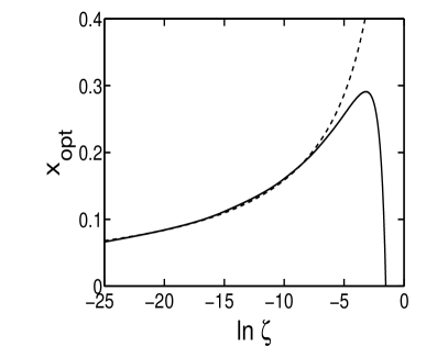
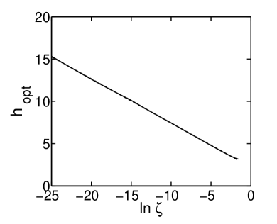
Figure 4.4: The optimal values $x_{\rm opt}$ and $h_{\rm opt}$ for the pairing interaction, Eq. (4.12). The dashed lines indicate the asymptotic behaviors, Eq. (4.13).

The accuracy of these approximations can be observed in Fig. 4.4 that shows the numerically computed optimal value $x_{\rm opt}(\zeta)$ [left panel] and the corresponding $h_{\rm opt}(\zeta)=h(x_{\rm opt},\zeta)$ [right panel] as a function of $\ln\zeta$ (solid lines), compared with the approximations above (dashed lines). One readily notices the very good agreement between both calculations, especially for $h_{\rm opt}$, for which already at $\zeta\approx\exp(-2)\approx 0.13$ the two curves become indistinguishable at this scale.

Taking all these facts into account, the value of the pairing gap under optimal conditions becomes

$$\ln\frac{\Delta_{1}}{c_{1}\mu_{F}}\rightarrow-\frac{m_{BF}^{2}}{m_{B}m_{F}}\;\frac{\big{[}\ln{\eta}\big{]}^{2}}{0.52022\big{[}\ln{\zeta}-4.3257\big{]}}\>.$$ (4.14)

This means that the position and value of the maximum induced interaction will depend logarithmically on the Fermi momentum.

We compare now the importance of this induced interaction with a possible direct fermion-fermion $p$-wave interaction, which at low density is given by [RDS90],

$$T_{F}^{(L=1)}(k_{F},k_{F};2\mu_{F})\approx\frac{4\hbar^{2}}{m_{F}}\frac{\mu_{F}}{E_{1}}\propto\rho_{F}\>,$$

where $E_{1}$ is the parameter characterizing 2D low-density $p$-wave scattering. As the boson mediated attraction, Eqs. (4.12,4.13), at low density depends only logarithmically on the fermion density, it will dominate in this limit. For the same reason, any fermionic polarization corrections can also be neglected.

Finally, we analyze the assumption $\mu_{B}\ll\mu_{F}$ used above. The boson chemical potential is determined by [Sch71, FH88, SB93, LMDB02]

$$\mu_{B}=\rho_{B}\textsf{T}_{\rm BB}(E=\mu_{B})=\frac{4\pi\hbar^{2}\rho_{B}}{m_{B}}\frac{1}{\ln{(E_{BB}/\mu_{B})}}\>,$$

while for free fermions we have

$$\mu_{F}=\frac{2\pi\hbar^{2}\rho_{F}}{m_{F}}\>.$$

Since the logarithm in the low-density domain is always large, we have the sufficient condition

$$\frac{2m_{F}}{m_{B}}\frac{\rho_{B}}{\rho_{F}}\lesssim 1\leavevmode\nobreak\ \leavevmode\nobreak\ \Rightarrow\leavevmode\nobreak\ \leavevmode\nobreak\ \frac{\rho_{F}}{\rho_{B}}\equiv x\gtrsim\frac{2m_{F}}{m_{B}}\>.$$

which will be well satisfied in atomic mixtures ($2m_{F}/m_{B}\sim 1$) in the regime of validity of (4.13).

4.3.3 Prospects of experimental detection

In order to estimate typical sizes of the expected gap, we plot in Fig. 4.5 the gap $\Delta_{1}/\mu_{F}$, according to Eq. (4.14), as a function of the parameters $\eta$ and $\zeta$ defined above (assuming for simplicity $c_{1}=1$). On the left we show the calculation for a ⁸⁷Rb-⁴⁰K mixture. We see that quite large gaps $\Delta_{1}\sim\mu_{F}$ are achievable, and that it is mainly $\eta\propto\varepsilon_{F}/E_{BF}$ that determines the size of the gap. Indeed, the lines of constant value of the gap are almost parallel to the $\zeta$ axis, as shown by the contour lines in the $\eta-\zeta$ plane, except for $\eta\gtrsim 0.1$, when the gap is already large ($\Delta_{1}/\mu_{F}\gtrsim 0.8$). On the right part of the figure, we compare these results for the ⁸⁷Rb-⁴⁰K mixture with the corresponding ones for a ⁷Li-⁶Li mixture. The general behavior is essentially the same, but the gap is a little bit smaller in the last case, the difference being due to the different value of the masses’ coefficient in Eq. (4.14), whose value is 0.22 for the first mixture and 0.25 for the second one. Even though this difference is small, the fact that appears in the exponential gives rise to the difference in the figure.

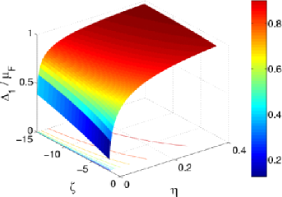
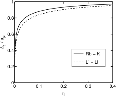
Figure 4.5: The pairing gap for optimal boson concentration, Eq. (4.14), as a function of $\eta=m_{BF}\varepsilon_{F}/(m_{F}E_{BF})$ and $\zeta=m_{F}\varepsilon_{F}/(m_{B}E_{BB})$: (left) for a ⁸⁷Rb-⁴⁰K mixture; (right) comparison with a ⁷Li-⁶Li mixture for fixed $\zeta$.

In summary, we expect quite large gaps $\Delta_{1}\lesssim\mu_{F}$ with fermion chemical potentials $\mu_{F}\lesssim E_{BF}$, while $E_{BB}$ should play a minor role.

In order to translate this condition into experimental quantities, we use the results of Refs. [PHS00, PS01, LMDB02], relating the 2D scattering parameter $E_{0}$ to the value of the 3D scattering length $a_{3D}$, for a system confined in a strongly anisotropic trap characterized by frequencies $\omega_{\perp}$ and $\omega_{z}\gg\omega_{\perp}$. Assuming that these frequencies are the same for the two trapped species, the treatment of [PS01] is equally valid for a mixture if we substitute the masses $m$ there by twice the reduced mass of the pair. Thus, for the boson-fermion collision parameter, we obtain

$$\frac{\mu_{F}}{E_{BF}}=\frac{\pi}{B}\frac{\mu_{F}}{\hbar\omega_{z}}\exp{\left(-\sqrt{2\pi}\frac{l_{z}}{a_{BF}}\right)}\>,$$ (4.15)

where $B\approx 0.915$ and $l_{z}=\hbar/\sqrt{2m_{BF}\omega_{z}}$. Since at the same time for a 2D situation the condition $\mu_{F}\ll\hbar\omega_{z}$ must be fullfilled, one can only expect observable gaps if the exponential term is not too small. We can distinguish two cases:

• $a_{BF}>0$: in this case the ratio $l_{z}/a_{BF}$ should be minimized as much as possible. One possibility is to strongly compress the trap in the $z$ direction, or even better use a one-dimensional optical lattice to divide the trapped gas in a set of quasi-2D sub-systems. Another option is using a Feshbach resonance to enhance the repulsion; in this case, problems of stability might appear, as for strong interspecies repulsions the system may prefer to spatially separate the two species.

• $a_{BF}<0$: in this case the exponential term is never small and pairing can be expected as long as $\mu_{F}/(\hbar\omega_{z})$ is not too small. Using the Thomas-Fermi approximation $\mu_{F}=\sqrt{2N_{F}}\hbar\omega_{\perp}$ for the chemical potential of a non-interacting, strictly two-dimensional Fermi gas in a (in-plane) harmonic trap of frequency $\omega_{\perp}$, this last condition can be expressed as

  $$\frac{\mu_{F}}{\hbar\omega_{z}}=\frac{\omega_{\perp}}{\omega_{z}}\sqrt{2N_{F}}\>.$$ (4.16)

  Let us take typical values from [LENS03], where around $5\times 10^{4}$ atoms of ⁴⁰K were sympathetically cooled with ⁸⁷Rb down to $T/T_{F}=0.3$ ($T_{F}=430$ nK) in a magnetic trap with frequencies $\omega_{z}=2\pi\times 317$ Hz, $\omega_{a}=2\pi\times 24$ Hz, and then submitted to an optical lattice with associated harmonic frequencies in the minima $\omega_{l}=2\pi\times 43$ kHz. Therefore $\omega_{\perp}/\omega_{z}\rightarrow\omega_{z}/\omega_{l}\approx 1/136$, and we get a value $\sim 2$ for the ratio in Eq. (4.16), which is close to the requirement for 2D behavior.

Let us note also that Eq. (4.15) applied to quasi-2D, bosonic ⁸⁷Rb trapped with the same $\omega_{z}$ as above gives $\mu_{F}/E_{BB}\propto\zeta\ll 1$, thus ensuring a broad range of $\mu_{F}/E_{BF}$ over which large gaps are expected (see Fig. 4.5).

4.4 Discussion

Under favorable circumstances, $p$-wave pairing gaps of the order of the Fermi energy seem to be achievable, and comparable to those predicted for $s$-wave pairing in quasi-2D two-component Fermi gases [PBS03]. However, more precise quantitative predictions cannot be made in this regime within the present approach since, when $\mu_{F}\approx\{E_{BF},E_{BB}\}$, also the asymptotic expression Eq. (4.9) becomes invalid. We stress that the same effect in three dimensions is less efficient in increasing the size of the gap, and one expects $\Delta_{1}/\mu_{F}\leq 0.1$ [HPSV00].

Also the stability of a Bose-Fermi mixture in two dimensions is as yet an unexplored subject. In three dimensions, this topic has been studied by different authors [M l98, VPS00, MSY01, RF02, PZWM02, SPZM02, Rot02, VG02] that reach similar conclusions. Here we briefly comment on the implications from these studies that might be applied to our case, but a more precise analysis of the two-dimensional case would be of high interest.

According to Ref. [VPS00], in a three-dimensional boson-fermion mixture one can expect to find one of the following situations:

• a fermionic phase and a bosonic phase, separated from each other;

• a fermionic phase and a boson-fermion mixture;

• a single uniform mixture.

In case (i) there is no boson-fermion induced interaction nor sympathetic cooling. In case (ii) these problems are overcome, but only a fraction of the fermions is efficiently cooled and can undergo the superfluid transition. Therefore, the interesting situation is that of case (iii). This can be obtained if there is attraction between bosons and fermions (to avoid their spatial separation), but in this case the system may collapse due to this same attraction as predicted in [RF02] and observed in [LENS02]. This will happen if, e. g., the number of bosons exceeds some critical number $N_{\rm cr}$, which will depend on $a_{BB}$ and $a_{BF}$. For a uniform system, we know that $a_{BB}>0$ is required in order to avoid the collapse of the bosonic component. Roth and Feldmeier have shown that this condition also stabilizes significantly the mixtures, even for $a_{BF}<0$, while the case $a_{BF}>0$ rapidly gives rise to spatial separation of the two components [RF02].

Applying these arguments to the mixtures used in typical atomic experiments, we see that the case ⁷Li-⁶Li with $a_{BB}=-1.5\;\rm nm$ and $a_{BF}=2.2\;\rm nm$ [Rice01] does not correspond to the optimal stability conditions. However, the presence of the trapping stabilizes the system so that experiments can be performed. On the other hand, for the ⁸⁷Rb-⁴⁰K mixture, where $a_{BB}=5.2$ nm [vKKHV02] and $a_{BF}=-22$ nm [LENS02], the stability conditions for the homogeneous case are fully satisfied.

In conclusion, the ⁸⁷Rb-⁴⁰K mixture seems to be the best available candidate within present-day ultracold boson-fermion mixtures to explore the outlined possibility of a $p$-wave superfluid transition in a (quasi)-2D system, both because of its demonstrated stability against phase separation and collapse, and because the expected gaps $\Delta_{1}\sim\mu_{F}$ are larger that those for ⁷Li-⁶Li mixtures.

Chapter 5 Dynamics of spin-1 condensates at finite temperatures

Fu mio padre il primo ad accorgersi che qualcosa stava cambiando. Io ero appisolato e il suo grido mi svegliò:
— Attenzione! Qui si tocca!
Sotto di noi la materia della nebula, da fluida che era sempre stata, cominciava a condensarsi.

Italo Calvino, Sul far del giorno (Le Cosmicomiche)

5.1 Introduction

In the previous chapters we have studied the prospects for a superfluid transition in a low density fermionic gas with two species of fermions (chapters 2 and 3) or in a mixture of a bosonic and a fermionic species (chapter 4). We will analyze now the behavior of another multicomponent system, this one with only bosonic components, namely a so-called spinor condensate.

We have seen in Section 2.1 how alkali atoms can be trapped by means of an inhomogeneous magnetic field. In this situation, the same magnetic field that traps the atoms by coupling to their magnetic moment, freezes their spin degree of freedom. Thus, the atoms behave in practice as spinless bosons, and the structure and dynamics of low density gases can be well described by the famous Gross-Pitaevskii equation for a scalar order parameter $\psi(\bm{r},t)=\langle\Psi(\bm{r},t)\rangle$ in an external potential $V_{\rm ext}$,

$$i\hbar\frac{\partial\psi(\bm{r},t)}{\partial t}=-\frac{\hbar^{2}}{2M}\nabla^{2}\psi(\bm{r},t)+V_{\rm ext}(\bm{r},t)\psi(\bm{r},t)+g|\psi(\bm{r},t)|^{2}\psi(\bm{r},t)\>,$$

with the coupling strength $g=4\pi\hbar^{2}a/M$ associated to a contact interaction with scattering length $a$ for particles of mass $M$ [Gro61, Pit61, DGPS99].

The situation is different when the atoms are trapped by means of an electric field interacting with their electric dipole moment, $\bm{d}$. Even if alkali atoms have ground states with vanishing $\bm{d}$, when they are placed in an electric field, they acquire an induced electric moment $\bm{d}\neq\bm{0}$. Its value is proportional to the electric field, with the proportionality constant given by the polarizability of the atom. In a first approximation, the polarizability is independent of the magnetic quantum number $m$ for atoms of the same hyperfine spin $f$ [Ho98]. Therefore, it is possible to store atoms in all the states $|f;m=-f,\cdots,f\rangle$ in an optical trap.

The experimental procedure is typically as follows: First, the atoms are trapped with a magnetic field. Then, a set of lasers is switched on, defining an optical trap superimposed to the magnetic one. Finally, the magnetic trap is switched off, and the atoms remain in the optical potential. The first realization of such a scheme was done by the group of W. Ketterle at mit in 1997 [MIT98a]. The remarkable degree of experimental control on lasers allows for a great capacity to modify the trap in a controlled way. In particular, it permits the production of very elongated traps, where quasi-one-dimensional atomic systems are realized.

The ability to build such optical traps led the Ketterle group to the production of the first spinor condensate with ²³Na atoms [MIT98b]. The ground state of ²³Na has total spin $f=1$ and the atoms can be in three hyperfine states, $m=-1,0,1$. In the first stage of the experiment, atoms in the $|f,m\rangle=|1,-1\rangle$ state —which is low magnetic field seeking— are magnetically trapped. Then, they are transferred to the optical trap, where arbitrary populations of the three states are prepared using radio-frequency transitions (Landau-Zener sweeps) [MIT98a]. Recently, similar experiments have been accomplished with ⁸⁷Rb atoms in Hamburg [Hamb04a], Georgia Tech [GaTe04], Gakushuin [Gaku04] and Berkeley [UCB05].

It is interesting to note also that spinor condensates are closely related to the pseudo-spin-1/2 systems realized in a purely magnetic trap by the group of Eric Cornell at jila since 1997 [JILA97, JILA98a, JILA98b]. In these experiments, ⁸⁷Rb atoms where trapped in the state $|f=1,m=-1\rangle$ and coupled via a two-photon transition to the state $|2,1\rangle$. Even though the states in the $f=2$ manifold are metastable, the lifetime of the system (a few seconds) is long enough to perform measurements. In such systems, remarkable results as spin waves at $T>T_{c}$ [JILA02] and decoherence effects [JILA03b] have been observed, as well as interlaced vortex lattices with orthorombic symmetry [JILA04c]. This surprising behavior, which contrasts with the ‘usual’ hexagonal Abrikosov lattices encountered in one-component atomic BECs, had been foreseen among others by Mueller and Ho [MH02] and by Kasamatsu et al. [KTU03]. Studies on vortex and spin textures for $f=1$ spinor condensates can be found in [Mue04] and [RvLSR02]. Other properties of two-component Bose-Einstein condensates studied in the literature are: collective modes [PB98, SC03, KTU04], spin structures in the ground and vortex states [HS96, FS01, RD05], solitons [OS01, BA01, KNF⁺04, Ruo04, Ber05], formation of spin domains [KT04] and Josephson-like oscillations [OS99, LdPL00, GPS02]. We finally quote also the experiments on cold gases with two different bosonic atoms by the group of M. Inguscio and G. Modugno at lens, who succesfully created a BEC of ⁴¹K atoms by sympathetic cooling with ⁸⁷Rb [LENS01]; other mixtures under study are Rb-Cs [Pisa05, And05], and Li-Cs [Heid01].

The theoretical study of integer-$f$ systems in the context of ultracold gases was initiated by T.-L. Ho [Ho98], Ohmi and Machida [OM98] and Law et al. [LPB98]. The correct treatment of the spin degrees of freedom of the individual atoms requires to consider the vectorial character of the field operator in spin space. In the mean-field approximation, this feature is transferred to the order parameter,

$$\langle{\vec{\Psi}}\rangle=\vec{\psi}=\left(\begin{array}[]{c}\psi_{f}\\ \psi_{f-1}\\ \vdots\\ \psi_{-f}\end{array}\right)=\left(\begin{array}[]{c}|\psi_{f}|e^{i\theta_{f}}\\ |\psi_{f-1}|e^{i\theta_{f-1}}\\ \vdots\\ |\psi_{-f}|e^{i\theta_{-f}}\end{array}\right)\>.$$ (5.1)

Alternatively, this can be interpreted as having a different order parameter for each spin projection.

An additional peculiarity of these systems is that spin-exchanging interactions allow for a transference of population between the different components $m=-f,\cdots,f$, subject only to the conservation of the total number of particles ${\cal N}=\sum_{m}N_{m}$ and of the magnetization of the system, defined as ${\cal M}=\sum_{m}m\times N_{m}$, being $N_{m}$ the number of atoms in the $m$ component. For instance, two atoms in the state $|f=1,m=0\rangle$ may collide and become two atoms in the states $|1,+1\rangle$ and $|1,-1\rangle$. Thus, the structure of the exact ground state, as well as the dynamics, will depend on the spin-dependent part of the Hamiltonian. In fact, it is the importance of the spin degree of freedom in these multicomponent systems that has awarded them the name spinor condensates, even if the term ‘spinor’ would not be rigorous from a purely mathematical point of view.

5.2 Formalism

As usual for ultracold gases, the low density and temperature of these systems allow to substitute the interatomic potential by a contact pseudopotential, characterized by its scattering length. To take into account the fact that a collision between two spin-$f$ atoms can happen in any of the channels of total spin $F=0,1,2,\cdots,2f$, this interaction is now written as

$$V=\delta(\bm{r}_{1}-\bm{r}_{2})\,\sum_{F=0}^{2f}g_{F}{\cal P}_{F}\>,$$ (5.2)

where ${\cal P}_{F}$ projects the two-particle state onto the subspace of total spin $F$, in which the coupling $g_{F}$ is related to the scattering length $a_{F}$ by $g_{F}=4\pi\hbar^{2}a_{F}/M$. Symmetry constrains $F$ to take even values for identical bosons, and odd values for identical fermions. Denoting by $\bm{f}_{i}$ the spin of atom $i=1,2$ in a collision, and using the identity $\bm{F}^{2}=(\bm{f}_{1}+\bm{f}_{2})^{2}$, we have

$$\bm{f}_{1}\cdot\bm{f}_{2}=\sum_{F=0}^{2f}\lambda_{F}{\cal P}_{F}\>,\qquad\lambda_{F}=\frac{F(F+1)-2f(f+1)}{2}\>,$$

where the summation over $F$ takes into account the possibility of the collisions occurring through different spin channels. This expression will be useful to substitute (some of) the projectors in Eq. (5.2) by products of atomic spin operators.

We will for definiteness present the results for the case of bosons with spin $f=1$ (for instance, ²³Na and ⁸⁷Rb in their electronic ground state), while more detailed calculations for both $f=1$ and $f=2$ are given in Appendix B. In this case, the previous expressions together with the normalization of the projectors, $\sum_{F}{\cal P}_{F}={\cal P}_{0}+{\cal P}_{2}=1$, allow us to write the potential as

$$V=c_{0}+c_{2}\,\bm{f}_{1}\cdot\bm{f}_{2}\>,$$

with the coupling strengths given by

$$c_{0} =\frac{g_{0}+2g_{2}}{3}=\frac{4\pi\hbar^{2}}{3M}\left(a_{0}+2a_{2}\right)\>,$$ (5.3a)

$$c_{2} =\frac{g_{2}-g_{0}}{3}=\frac{4\pi\hbar^{2}}{3M}\left(a_{2}-a_{0}\right)\>.$$ (5.3b)

Thus, the interaction has a spin-independent part ($\propto c_{0}$) and a contribution ($\propto c_{2}$) that couples atoms with different magnetic quantum numbers $m$, keeping constant the total value $M=m_{1}+m_{2}$ for the pair. We remark that this potential is invariant under rotations $R(\alpha,\beta,\gamma)$ in spin space, where $\{\alpha,\beta,\gamma\}$ denote the Euler angles defining the rotation (see Fig 5.1).

Figure 5.1: The Euler angles $\{\alpha,\beta,\gamma\}$ that define a rotation from the coordinate system $xyz$ to $x^{\prime}y^{\prime}z^{\prime}$.

Once the potential is defined, we can write down the Hamiltonian in second-quantized form:

$$H=\int\mathrm{d}^{3}r\left\{\Psi^{\dagger}_{m}\left(-\frac{\hbar^{2}}{2M}{\bm{\nabla}}^{2}+V_{\rm ext}\right)\Psi_{m}\right.\\ \left.+\frac{c_{0}}{2}\Psi^{\dagger}_{m}\Psi^{\dagger}_{j}\Psi_{j}\Psi_{m}+\frac{c_{2}}{2}\Psi^{\dagger}_{m}\Psi^{\dagger}_{j}{\bm{F}}_{mk}\cdot{\bm{F}}_{jl}\Psi_{l}\Psi_{k}\right\}\>,$$ (5.4)

where $\Psi_{m}(\bm{r})$ $(\Psi_{m}^{\dagger}(\bm{r}))$ is the field operator that annihilates (creates) an atom in the hyperfine state $|f=1,m=1,0,-1\rangle$ at point $\bm{r}$, and summation over repeated indices is to be understood. The trapping potential $V_{\rm ext}(\bm{r})$ is assumed harmonic and spin independent. Finally, $\bm{F}$ denotes the vector of spin-1 Pauli matrices [Ho98, ZYY04]

$$F_{x}=\frac{1}{\sqrt{2}}\left(\begin{array}[]{ccc}0&1&0\\ 1&0&1\\ 0&1&0\\ \end{array}\right),\leavevmode\nobreak\ \leavevmode\nobreak\ F_{y}=\frac{1}{i\sqrt{2}}\left(\begin{array}[]{ccc}0&1&0\\ -1&0&1\\ 0&-1&0\\ \end{array}\right),\leavevmode\nobreak\ \leavevmode\nobreak\ F_{z}=\left(\begin{array}[]{ccc}1&0&0\\ 0&0&0\\ 0&0&-1\\ \end{array}\right).$$

5.2.1 Ground state of the homogeneous system

Let us first consider the case of a homogeneous system from a mean-field point of view: we substitute the field operators $\Psi_{m}$ by their expectation values $\psi_{m}$. Let us also define the spin components $\xi_{m}$ of the mean-field order parameter through

$$\vec{\psi}:=\left(\begin{array}[]{ccc}\psi_{1}\\ \psi_{0}\\ \psi_{-1}\end{array}\right)\equiv\sqrt{n}\left(\begin{array}[]{ccc}\xi_{1}\\ \xi_{0}\\ \xi_{-1}\end{array}\right)\>,$$ (5.5)

where $n$ is the total density of the system and $\sum_{m}|\xi_{m}|^{2}=1$. The general form to describe a state of a homogeneous spin-1 system with magnetization $\cal M$ is

$$\vec{\xi}=e^{i\theta}\left(\begin{array}[]{c}e^{-i\phi}\sqrt{\frac{1-|\xi_{0}|^{2}+\cal M}{2}}\\ \rule[-12.91663pt]{0.0pt}{30.00005pt}|\xi_{0}|\\ e^{i\phi}\sqrt{\frac{1-|\xi_{0}|^{2}-\cal M}{2}}\end{array}\right)\>,$$

where $\theta$ and $\phi$ are arbitrary phases, and $|\xi_{0}|\in\mathbb{R}$ is a free parameter.

The interaction part of the Hamiltonian reads

$$H_{\rm int} =\int\mathrm{d}^{3}r\frac{n^{2}}{2}\left[c_{0}+c_{2}\langle\bm{F}\rangle^{2}\right]\>,$$

$$\langle\bm{F}\rangle :=\sum_{kl}\xi_{k}^{*}\bm{F}_{kl}\xi_{l}\>.$$

Therefore, the spin structure of the ground state is determined by the sign of $c_{2}\propto a_{2}-a_{0}$:

• $c_{2}>0$: the energy is minimized by setting $\langle\bm{F}\rangle=0$, and the system is usually called ‘antiferromagnetic’ [Ho98]. An analogy with condensed-matter antiferromagnetism is to be taken with care as there the interaction $\bm{f}_{1}\cdot\bm{f}_{2}$ is typically between spins in different positions of space, which implies a spatial ordering of them, while here the interaction is local. An example of atom with ‘antiferromagnetic’ interactions is ²³Na in the $f=1$ manifold.

  This structure for the ground state is achieved in the state $\vec{\xi}^{\,T}=(0,1,0)$ ($T$ denotes transpose) or more generally, due to rotational symmetry in spin space, in any of the states

  $$\vec{\xi}_{AF}=e^{i\theta}\left(\begin{array}[]{c}-\frac{1}{\sqrt{2}}e^{-i\alpha}\sin\beta\\ \cos\beta\\ \frac{1}{\sqrt{2}}e^{i\alpha}\sin\beta\end{array}\right)\>,$$

  where $\theta$ is a global phase that does not affect any expectation value, and $\{\alpha,\beta\}$ are the Euler angles that fix the quantization axis. This ground state presents a $U(1)\times S^{2}$ symmetry and is usually referred to as a polar ground state [Ho98].

• $c_{2}<0$: the energy is minimized by setting $|\langle\bm{F}\rangle|=1$, and the system is called ‘ferromagnetic’ [Ho98]. The ground state configuration of the spin components reads

  $$\vec{\xi}_{F}=\left(\begin{array}[]{c}1\\ 0\\ 0\end{array}\right)\sim\leavevmode\nobreak\ e^{i(\theta-\gamma)}\left(\begin{array}[]{c}e^{-i\alpha}\cos^{2}\frac{\beta}{2}\\ \sqrt{2}\cos\frac{\beta}{2}\sin\frac{\beta}{2}\\ e^{i\alpha}\sin^{2}\frac{\beta}{2}\\ \end{array}\right)\>.$$

  Note the coupling of the Euler angle $\gamma$ to the global phase $\theta$. The symmetry is now $SO(3)$ [Ho98].

A similar treatment follows for larger spin values, the main difference being the greater number of scattering parameters that enter into the play and, thus, the richer phase diagram that emerges. For instance, the case of $f=2$ has been studied by Ciobanu et al., who show that there are 3 possible phases for the ground state depending on the values of the couplings $c_{0}\propto 4a_{2}+3a_{4}$, $c_{1}\propto 7a_{0}-10a_{2}+3a_{4}$ and $c_{2}\propto a_{4}-a_{2}$ [CYH00] (see also [KU00]).

It is also worth noticing that the presence of a homogeneous magnetic field can drastically affect the structure of the ground state, as was analyzed by Zhang et al. for the case of $f=1$ [ZYY03] and for $f=2$ by Ciobanu et al. [CYH00] and more recently by Saito and Ueda [SU05b]. Also the dynamics of the system is strongly influenced by external magnetic fields as studied theoretically for the case of spin 2 by Saito and Ueda [SU05a], and shown experimentally by the Hamburg [Hamb04b] and Gakushuin [Gaku04] groups. This notwithstanding, in order to reduce the number of parameters entering our simulations and thus have a clearer picture of the effects of temperature, we will restrict our analysis to the case of a vanishing magnetic field.

5.2.2 Dynamical equations and transfer of population

We focus now on the dynamical evolution of a trapped $f=1$ condensate and, in particular, on the possible influence on it of thermal effects. In experiments, practically any initial configuration $\bm{N}(t=0)=(N_{1},N_{0},N_{-1})$ can be produced, and it is interesting to analyze e. g. whether the system is expected to converge in the time scale of an experiment to its ground-state configuration, or the spin structures that can appear in the dynamical process.

The equations of motion for the mean-field order parameters can be derived from the energy expression in a mean-field formulation,

$${\cal E}[\vec{\psi}]=\int\mathrm{d}^{3}r\,\bigg{\{}\psi^{*}_{m}\left(-\frac{\hbar^{2}}{2M}{\bm{\nabla}}^{2}+V_{\rm ext}\right)\psi_{m}\\ +\frac{c_{0}}{2}\psi^{*}_{m}\psi^{*}_{j}\psi_{j}\psi_{m}+\frac{c_{2}}{2}\psi^{*}_{m}\psi^{*}_{j}{\bm{F}}_{mk}\cdot{\bm{F}}_{jl}\psi_{l}\psi_{k}\bigg{\}}\,,$$ (5.6)

by functional differentiation according to $i\hbar\partial\psi_{m}/\partial t=\delta{\cal E}/\delta\psi_{m}^{*}$. One readily obtains (see Appendix B for details) [PLR⁺99, ZYY03]

$$i\hbar\frac{\partial\psi_{m}}{\partial t}=\left[-\frac{\hbar^{2}}{2M}{\bm{\nabla}}^{2}+V^{\rm eff}_{m}\right]\psi_{m}+c_{2}T_{m}^{*}\,,$$ (5.7)

where we have defined the transference terms

$$\left.\begin{array}[]{c}T^{*}_{\pm 1}=\psi_{0}^{2}\psi_{\mp 1}^{*}\>,\\ T^{*}_{0}=2\psi_{1}\psi_{0}^{*}\psi_{-1}\end{array}\right.$$ (5.8)

which render these equations different from the usual number-conserving Gross-Pitaevskii equation for one-component condensates. In fact, the $c_{2}$-term in the Hamiltonian does not couple directly the different $|f,m\rangle$ states in which one atom can be found —as the radio-frequency field couples the $|1,-1\rangle$ and $|2,1\rangle$ states in the jila experiments—, but the two-atom states $|Z\rangle:=|f_{1},m_{1}\rangle|f_{2},m_{2}\rangle=|1,0\rangle|1,0\rangle$ and $|U\rangle:=|1,1\rangle|1,-1\rangle$ (properly symmetryzed). The effective potentials that will determine the spatial dynamics of each component read

$$\left.\begin{array}[]{r@{}c@{}l}V^{\rm eff}_{\pm 1}&=&V_{\rm ext}+c_{0}n+c_{2}\left(\pm n_{1}+n_{0}\mp n_{-1}\right)\\ V^{\rm eff}_{0}&=&V_{\rm ext}+c_{0}n+c_{2}(n_{1}+n_{-1})\end{array}\right.\,,$$ (5.9)

with $n_{m}(\bm{r})=|\psi_{m}(\bm{r})|^{2}$ being the density of atoms in the $|1,m\rangle$ state and $n(\bm{r})=\sum_{m}n_{m}(\bm{r})$ the total density, normalized to the total number of atoms ${\cal N}$. The population of the hyperfine state $|1,m\rangle$ is $N_{m}=\int\mathrm{d}^{3}r\,|\psi_{m}|^{2}$, and $N_{1}+N_{0}+N_{-1}\equiv{\cal N}$ is a constant of the motion.

In analogy to what happens for the Gross-Pitaevskii equation of a spin-polarized condensate [DGPS99], equations (5.7) can be rewritten in the form of continuity equations, but now a balance term accounting for the transfer of populations between the components will appear on the right-hand side. Indeed, with the usual definition of the quantum current applied to each component,

$$\bm{j}_{m}=\frac{\hbar}{2iM}(\psi_{m}^{*}{\bm{\nabla}}\psi_{m}-\psi_{m}{\bm{\nabla}}\psi_{m}^{*})\>,$$

one readily finds

$$\frac{\partial n_{m}}{\partial t}+{\bm{\nabla}}\cdot\bm{j}_{m}=\delta\dot{n}_{m}(\bm{r},t)\,,\\$$ (5.10)

where $\delta\dot{n}_{m}(\bm{r},t)=-(2c_{2}/\hbar)\,{\rm Im}[T_{m}\psi_{m}]$ is the transfer of populations between spin components per unit time.

The dynamical equations for $m=\pm 1$ are invariant under time-reversal symmetry; therefore, $\delta\dot{n}_{1}=\delta\dot{n}_{-1}$, and the conservation of magnetization implies $\delta\dot{n}_{0}=-2\delta\dot{n}_{\pm 1}=(2c_{2}/i\hbar)\,(\psi_{1}\psi_{0}^{*2}\psi_{-1}-\psi_{1}^{*}\psi_{0}^{2}\psi_{-1}^{*})$.

5.3 Numerical procedure

We have studied a system of ⁸⁷Rb atoms in their electronic ground state manifold $f=1$, trapped in a very elongated trap as in the Hamburg experiment [Hamb04b]. In particular, we have considered 20 000 atoms confined in a trap characterized by frequencies $\omega_{\perp}=891$ Hz and $\omega_{z}=21$ Hz, which results in an aspect ratio $\omega_{z}/\omega_{\perp}=0.024\ll 1$. For this atom, $a_{2}=100.4a_{B}$ and $a_{0}=101.8a_{B}$ [vKKHV02], which results in $c_{2}<0$, and the expected behavior is ‘ferromagnetic’. Moreover, we have simulated a purely one-dimensional system in a trap of frequency $\omega_{z}$, as it has been shown that elongated spin-1 systems can be safely considered one-dimensional for most purposes [ZY05].

We have solved Eqs. (5.7) and analyzed them in terms of the transference terms (5.8) and the effective potentials (5.9). To this end, at each time step $dt$ we have split the evolution in two parts: the kinetic energy part, and the rest of the Hamiltonian. The evolution due to the kinetic energy has been solved by transforming the wave function into momentum space by a Fast Fourier Transform subroutine, and then the operator $\exp[-ip^{2}/(2m)\,dt]$ has been applied to it. Finally, the wave function is transformed back into real space, where the effect of the trapping potential and the coupling terms has been taken into account by means of a fourth order Runge-Kutta algorithm. This splitting of the full evolution in two parts introduces, in principle, higher order terms when the separate parts do not commute with each other [see Eq. (6.12)]. However, for short enough time steps $dt$, these terms can be neglected. To check the accuracy of our procedure, we also solved the evolution entirely with the Runge-Kutta algorithm, computing the gradient terms numerically in $r$-space: both methods give the same results for the test cases analyzed, but the split method can make use of much larger time steps and, thus, calculations are faster.

We consider that initially a quasi-pure condensate in the $m=0$ spin component is populated. Numerically, spin mixing requires at least a small seed of atoms populating the other components, but we keep the total magnetization equal to zero for the following reason: It has been shown that, for the case of zero magnetization, not all the phases $\theta_{m}$ in Eq. (5.1) affect the spin dynamics, but it is governed by only one relative phase $\Theta=2\theta_{0}-\theta_{1}-\theta_{-1}$ [PLR⁺99]. Therefore, we set $\theta_{1}=\theta_{-1}=0$ and vary only $\theta_{0}$. This relative phase is a very important parameter, as it can freeze completely the spin dynamics, or make it faster or slower [PLR⁺99]. In the experimental scheme, the phases are not well controlled, and vary from shot to shot. Thus, in order, to reproduce experimental results, we will randomly draw 20 values for $\Theta$ in the range $[0,2\pi)$, and make an average of the corresponding results.

5.4 Dynamical evolution at zero temperature

First of all, we perform several simulations at zero temperature, to be compared with the work of Yi et al. [YMSY02]. These authors work in the so-called Single Mode Approximation (sma) which, based on the fact that $|c_{2}|\ll c_{0}$, assumes $\xi_{m}(\bm{r})=\xi_{m}$ [PLR⁺99]. This approximation allows for some analytical insight into the properties of condensates with spin degree of freedom, and has therefore been extensively used. However, its accuracy was analyzed by Pu et al. [PLR⁺99], who established that it is only adequate for small particle numbers, when the contribution from the $c_{2}$ term is negligible. As ${\cal N}$ increases, the contribution from the spin-exchange term is more and more relevant and the sma becomes invalid. In our system, ${\cal N}=2\times 10^{4}$ and we have checked that indeed the density profiles for the different components cannot be transformed into one another by a simple rescaling, i. e. $n_{m}(\bm{r})/n_{m^{\prime}}(\bm{r})\not=\mbox{ constant }\forall\bm{r}\leavevmode\nobreak\ (m\neq m^{\prime})$ (see Figs. 5.3 and 5.6 below). Therefore, we will not use the sma in our work.

The results of our simulations at zero temperature are summarized in Figs. 5.2–5.4. In figure 5.2 we plot the population of each spin component as a function of time, for the initial populations $(N_{1}/{\cal N},N_{0}/{\cal N},N_{-1}/{\cal N})=(0.5\%,99\%,0.5\%)$.

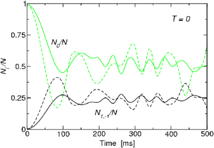
Figure 5.2: Population of the spin components as a function of time for the initial configuration $(N_{1}/{\cal N},N_{0}/{\cal N},N_{-1}/{\cal N})=(0.5\%,99\%,0.5\%)$ and $T=0$: the light, green lines stand for $N_{0}(t)$, while the dark, black lines are $N_{\pm 1}(t)$. The results obtained with one initial phase $\Theta=0$ are denoted by dashed lines, while solid lines show numerical results averaged over 20 random initial relative phases $\Theta$.

Dashed lines correspond to the dynamical evolution with an initial relative phase $\Theta=0$, and solid lines stand for the average over $20$ random initial relative phases. In absence of a magnetic field gradient the dynamical evolution of the $m=\pm 1$ spin components is the same, and the curves $N_{1}(t)$ and $N_{-1}(t)$ coincide; besides $\sum N_{m}(t)={\cal N}$ is always fulfilled.

For the case of fixed $\Theta=0$ (dashed lines), we observe several oscillations of the populations as a function of time, with a period $\tau\sim 50$ ms. These oscillations are reminiscent of Josephson oscillations between the two-atom states $|1,0\rangle|1,0\rangle$ and $|1,1\rangle|1,-1\rangle$, coupled by the $c_{2}$-term of the Hamiltonian, but appear to be damped. We have checked that these oscillations are coherent in a homogeneous system, i. e., after a certain period $\tau_{J}\approx\hbar/(c_{2}\overline{n})\approx 50$ ms ($\overline{n}=10^{14}$ cm^-3) one has $\bm{N}(t=\tau_{J})=\bm{N}(t=0)$, while at $t=\tau_{J}/2$ the populations are reversed, $N_{\pm 1}(t=\tau_{J}/2)=N_{0}(0)/2$ and $N_{0}(t=\tau_{J}/2)=2N_{\pm 1}(0)$. In the case of the trapped gas, the inherent nonlinear character of the interacting system, together with the discreteness of its spectrum, induce a ‘collapse’ [ENS80, MCWW97] or ‘dephasing’ [VL99, Leg01, OL02] of the oscillations. Moreover, as the period of oscillation depends strongly on the relative phase $\Theta$, an average over various values induces a further reduction of the amplitude of the oscillations, as shown by the solid lines in the figure. At much longer times, it has been shown that the full quantum solution presents revivals of the exchange of populations [PLR⁺99]. Nevertheless, this result cannot be retrieved in a mean-field calculation such as ours [MCWW97].

In both our calculations (with or without average), the magnetization ${\cal M}=\sum_{m}m\times N_{m}$ is conserved during the time evolution, as it has been experimentally observed [GaTe04]. The oscillations between the populations of the $m=0$ and $m=\pm 1$ states are not fully coherent but present a dynamical instability around $t\sim 100$ ms, when the large amplitude oscillations become small amplitude oscillations [SU05b]. At this point, the populations start to oscillate around the ground state configuration of the system with zero magnetization which, in absence of an applied magnetic field, is $(25\%,50\%,25\%)$ [ZYY03]. We note that these numerical results are in qualitative agreement with the experimental measurements of Ref. [GaTe04] obtained in a strongly anisotropic disk-shaped trap, where the relaxation to the steady state is also not monotonic but presents a few damped oscillations.

To further understand the spin dynamics, we now analyze the time evolution of the density profiles of the different spin components in the trap, in search for the possible existence of spin waves or the formation of spin domains. We plot the evolution corresponding to the run with fixed $\Theta=0$ in Fig. 5.3.

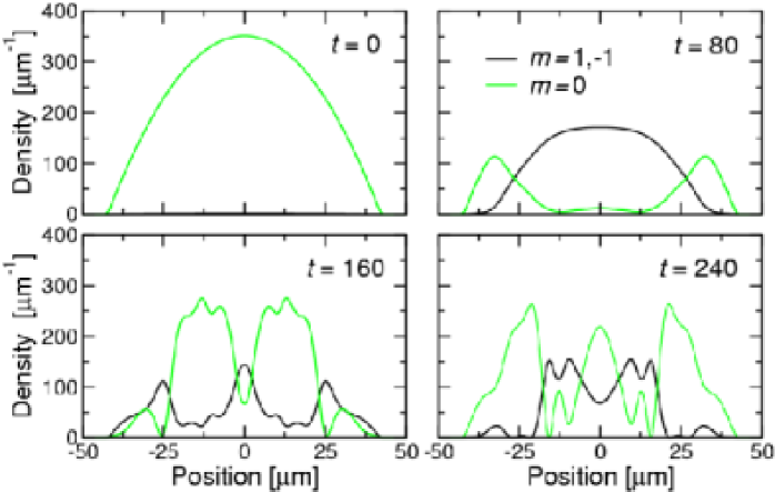
Figure 5.3: Density profiles of the spin components at the times indicated (in ms) and $T=0$, with the same color labelling as in Fig. 5.2. The initial configuration corresponds to $\bm{N}(t=0)/{\cal N}=(0.5\%,99\%,0.5\%)$, and $\Theta=0$ (dashed lines in Fig. 5.2).

At the initial stages of the evolution, the population of the $m=0$ component decreases due to the spin-exchange interaction, and the $\pm 1$ spin components start to be populated by equal amounts, keeping the magnetization of the initial state. In fact, the magnetization is locally conserved along the time evolution, a fact not required by the symmetries of the Hamiltonian.

For times $t<100$ ms, the conversion of atoms from $m=0$ to $m=\pm 1$ occurs mainly in the central part of the condensate, where the density is higher and thus the coupling among the different spin components is more effective, see Eq. (5.9). Later, at the time when the dynamical instability sets in, the $\pm 1$ spin components swing back to the $0$ component, giving rise to the formation of a spin structure with small domains. The $m=0$ and the $m=\pm 1$ domains are miscible, forming what can be named as ‘mixed domains’. This fact is related to the ‘ferromagnetic’ character of the interaction: if in the $m=\pm 1$ domains the spin is locally oriented (anti)parallel to the quantization axis, and in the $m=0$ domains it is perpendicular to it, in these ‘mixed domains’ the spin is locally oriented along a direction neither fully parallel nor perpendicular to the quantization axis. Thus, the succession of domains should reflect a smooth twist of the spin along the system, as also suggested by [SU05b].

The identical location of the $m=\pm 1$ domains is due to the symmetry in the corresponding initial profiles, together with the fact that the dynamical equations are symmetric under the relabelling $1\leftrightarrow-1$. Note also that the number of small spin domains does not grow indefinitely, but it is limited by a characteristic size $l_{\rm dom}$ that depends on the internal coupling between different spin components. We remark that the total density profile is constant during all the simulation, as expected for a trapped condensate in the Thomas-Fermi regime. Indeed, in this regime the spin-independent interaction $\sim c_{0}n\sim 100$ nK is dominant over the kinetic energy terms, thus preventing the formation of total-density modulations [HDR⁺01].

It has been argued that the appearance of the small domains is intimately related to a dynamical instability of the system. Therefore, the time scale of this process can be estimated from an analysis of the spectrum of the system. For two-component condensates, Kasamatsu and Tsubota [KT04] have observed a very fast appearance of structure in the spin density distribution of a ²³Na system. They estimate the time for the growth of domains as $\tau_{\rm growth}=2\pi/|\Omega_{-}|$, where $\Omega_{-}$ is the excitation frequency with largest imaginary part. In their case, $\tau_{\rm growth}\approx 25$ ms.

A similar analysis for $f=1$ condensates has been recently presented by Zhang et al. [GaTe05b]. For the case of ‘ferromagnetic’ interactions, the instability is expected to emerge at times $\sim 2\pi\hbar/(|c_{2}|n)$. For ⁸⁷Rb at densities $n\sim n(z=0)\approx 5\times 10^{14}$ cm^-3, this estimation is around 80 ms, which is in fair agreement with our results, cf. Fig. 5.3. They also estimate the typical size of a spin domain at long times as $\lambda_{\rm dom}=2\pi/k_{\rm inst}$, where $k_{\rm inst}$ is the highest momentum for which an unstable mode exists [i. e., Im$\,\omega(k_{\rm inst})\neq 0$]. With this formula, they get $\lambda_{\rm dom}\approx 13\leavevmode\nobreak\ \mu$m, a value consistent with our results. For ‘antiferromagnetic’ systems such as $f=1$ ²³Na, they predict no instability and, therefore, no domain formation, a point that we will address in Sect. 5.5.3.

It is possible to interpret the dynamical evolution of the various spin components in terms of the effective potential $V^{\rm eff}_{m}(z,t)$ felt by each one and through the continuity equations (5.10). To this end, we plot in Fig. 5.4 the effective potentials $V^{\rm eff}_{0}$ and $V^{\rm eff}_{1}=V^{\rm eff}_{-1}$ [top panels], and the local transfer of population $\partial_{t}n_{0}(z,t)$ and $\partial_{t}n_{1}(z,t)=\partial_{t}n_{-1}(z,t)$ [bottom panels] at times $t=$0, 40 and 80 ms, for the same initial conditions as in Fig. 5.3.

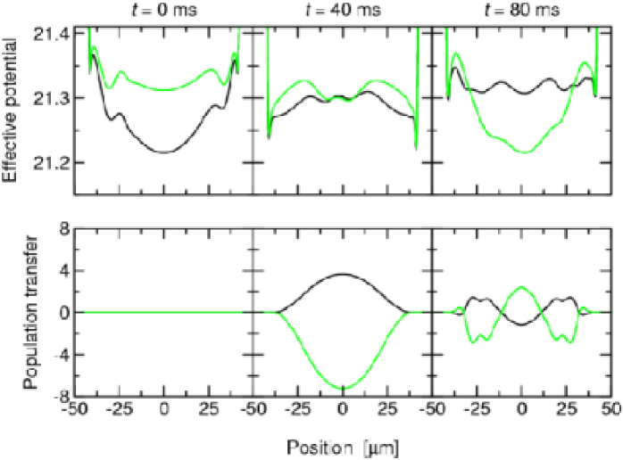
Figure 5.4: Effective potentials $V^{\rm eff}_{m}(z,t)$ in kHz [top] and population transfers $\delta\dot{n}_{m}(z,t)$ in $\mu$m${}^{-1}\cdot$ms^-1 [bottom] at $T=0$ for the initial configuration $\bm{N}(t=0)/{\cal N}=(0.5\%,99\%,0.5\%)$ and $\Theta=0$ (dashed lines in Fig. 5.2), at times $t=0$, 40 and 80 ms.

As is clear in Eq. (5.10), $\partial_{t}n_{m}$ has two contributions. For a fixed time, $\delta\dot{n}_{m}(z,t)$ represents the local variation in the occupation of the $|1,m\rangle$ state due to spin-exchanging collisions, while $-\bm{\nabla}\cdot\bm{j}_{m}$ takes into account the change in $n_{m}$ due only to motion of $m$-atoms. At the initial stages of the evolution, $t\lesssim 40$ ms, the densities of the $m=\pm 1$ components are very small and the dominant contribution is $\delta\dot{n}_{m}$ for all components. For example, at $t=40$ ms $\delta\dot{n}_{0}(z,t)<0$ and consequently $\delta\dot{n}_{1}(z,t)=\delta\dot{n}_{-1}(z,t)>0$: the $c_{2}$-term in the Hamiltonian is favoring the conversion of $|1,0\rangle|1,0\rangle$ pairs into $|1,1\rangle|1,-1\rangle$, as seen in Fig. 5.2 for the first stages of the evolution. At $t=0$ this is also true, but it cannot be appreciated from the scale of the figure. Moreover, since the minimum and maximum of $\delta\dot{n}_{0}(z,t)$ and $\delta\dot{n}_{\pm 1}(z,t)$, respectively are at the center of the condensate, the spin-exchange mainly occurs at the central region, as we have already observed in Fig. 5.3.

At $t=80$ ms $\delta\dot{n}_{\pm 1}$ is positive at the boundaries of the condensate, and negative in the central region, whereas $\delta\dot{n}_{0}$ has the opposite behavior. Therefore, the population with $m=\pm 1$ is converting into $m=0$ atoms at the center while still increasing at the boundaries. In fact, at this time, the total tranfers $\Delta\dot{N}_{m}(t)=\int\mathrm{d}z\,\delta\dot{n}_{m}(z,t)$ between $m=0$ and $m=\pm 1$ almost balance, which is reflected in the vanishing slope of the curves $N_{m}(t)$ of Fig. 5.2. At this stage of the evolution, the population of the $m=\pm 1$ states starts to be relevant, and the contribution of the currents is no longer negligible. Typically, it has the same sign as the spin-exchange contribution, but it is smaller in magnitude.

These features can also be understood in energy terms from the panels showing the effective potentials. For example, at $t=0$ the higher energy for the $m=0$ atoms induces them to convert into $m=\pm 1$ pairs, especially in the center of the cloud, where the difference $V^{\rm eff}_{0}-V^{\rm eff}_{\pm 1}$ is larger. At time $t=40$ ms, $V^{\rm eff}_{0}=V^{\rm eff}_{\pm 1}$ at the center and, therefore, the transfer of atoms will slow down there and reverse its sense shortly after, while the population of the $\pm 1$ components will continue to grow on the sides of the cloud (cf. Fig. 5.3). Later on, at $t=80$ ms, the energy of the $m=0$ component is still larger on the boundaries than that of the $m=\pm 1$ components, but it has become smaller in the center of the trap; therefore, 0-atoms will continue to convert into $\pm 1$-atoms in the boundaries, but the reverse will happen at the center, as confirms the lower panel.

5.5 Dynamical evolution at finite temperature

5.5.1 Introducing temperature fluctuations

We would like now to analyze if thermal effects may have some noticeable effect on the dynamics of spinor condensates, making their expected evolution differ from the results found in the previous section for $T=0$.

For single-component condensates, temperature effects on the condensate fraction, dynamics, and damping of excitation modes have been studied extensively. Usually, at low enough temperatures, thermal excitations can be accounted for within the Bogoliubov-de Gennes (bdg) [dG66, NP90] or Hartree-Fock-Popov (hfp) [ZNG99] frameworks. Recently, this last scheme has been applied to study finite temperature effects in the equilibrium density distribution of the condensed and non-condensed components of $f=1$ atoms optically trapped [ZYY04]. In our work, we will make use of the bdg theory to describe the thermal clouds present in multicomponent condensates.

For a highly elongated one-component system, it has been shown that at low temperatures thermal fluctuations are relevant in the phases of the field operator, while they can be disregarded on the density profile of the ground state [KK65, RC65]. To be precise, three regimes can be identified [PSW00], according to the value of the temperature relative to the degeneracy temperature $T_{\rm deg}={\cal N}\hbar\omega$ [KvD96] and a critical temperature for phase fluctuations $T_{\theta}=T_{\rm deg}\hbar\omega/\mu$: (a) a true condensate (density and phase fluctuations are small in the ground state) at $T\ll T_{\theta}$; (b) a quasicondensate for $T_{\theta}\ll T\ll T_{\rm deg}$: the density has the same profile as for the true condensate, but the phase fluctuates on scales smaller than the cloud size, and the coherence properties of the phase are drastically modified; (c) finally, for $T\gtrsim T_{\rm deg}$, both phase and density fluctuate, and the system is no longer quantum degenerate.

In the case of a one-dimensional, harmonically trapped single-component condensate, the Bogoliubov-de Gennes equations for the low-lying excitations,

$$\epsilon_{j}u_{j} =\left(-\frac{\hbar^{2}}{2m}\nabla^{2}+V_{\rm ext}-\mu+2gn\right)u_{j}+gn_{0}v_{j}$$ (5.11)

$$-\epsilon_{j}v_{j} =\left(-\frac{\hbar^{2}}{2m}\nabla^{2}+V_{\rm ext}-\mu+2gn\right)v_{j}+gn_{0}u_{j}\>,$$ (5.12)

can be solved exactly [Str98], obtaining the corresponding energy eigenvalues $\epsilon_{j}=\sqrt{j(j+1)/2}\,\hbar\omega$ and wave functions. These can be written in terms of Legendre polynomials as

$$f_{j}(z)=u_{j}(z)+v_{j}(z)=\left\{\frac{2j+1}{R_{\rm TF}}\frac{\mu}{\epsilon_{j}}\left[1-\left(\frac{z}{R_{\rm TF}}\right)^{2}\right]\right\}^{1/2}\!P_{j}\!\left(\frac{z}{R_{\rm TF}}\right)\>,$$

with the chemical potential given by $\mu=\hbar\omega(3{\cal N}\alpha/\sqrt{32})^{2/3}$, where $\alpha$ gives a measure of the strength of the interactions as compared to the trapping potential energy [PSW00], and $R_{\rm TF}=\sqrt{2\mu/m}/\omega$ is the Thomas-Fermi radius of the initial condensate.

As the density fluctuations with respect to the equilibrium profile $n_{\rm eq}(z)$ may be disregarded, one can write $\Psi(z,0)=\sqrt{n_{\rm eq}(z)}\exp[i\hat{\theta}(z)]$ for the particle anihilation operator, with the phase operator given by [PSW00]

$$\hat{\theta}(z)=\frac{1}{\sqrt{4n_{\rm eq}(z)}}\sum_{j}f_{j}(z)\hat{a}_{j}+{\rm H.c.}\>,$$

where $\hat{a}_{j}$ anihilates a quasiparticle in mode $j$. Thus, in the temperature range $T_{\theta}\ll T\ll T_{\rm deg}$, where only phase fluctuations are relevant, one can simulate the thermal fluctuations in a one-dimensional condensate by generating a thermal phase $\theta^{\rm th}(z)$ according to

$$\theta^{\rm th}(z)=\sum_{j=1}^{\infty}\left\{\frac{2j+1}{R_{\rm TF}}\frac{\mu}{\epsilon_{j}}\left[1-\left(\frac{z}{R_{\rm TF}}\right)^{2}\right]\right\}^{1/2}\frac{a_{j}+a_{j}^{*}}{\sqrt{4n_{\rm eq}(z)}}\,P_{j}\!\left(\frac{z}{R_{\rm TF}}\right)$$

and adding it to the mean-field order parameter before the real-time simulation starts [Hamb01, KSS⁺03]. An analogous treatment for the case of a multicomponent condensate shows that, assuming that initially almost all the atoms are in a single component, the bdg equations for the non-condensate atoms depend mainly on the excited fraction in this most populated hyperfine state. Therefore, one can simulate again temperature effect by introducing one such fluctuating phase for each spin component,

$$\theta^{\rm th}_{m}(z)=\sum_{j=1}^{\infty}\left\{\frac{2j+1}{R_{\rm TF}}\frac{\mu}{\epsilon_{j}}\left[1-\left(\frac{z}{R_{\rm TF}}\right)^{2}\right]\right\}^{1/2}\frac{a_{j}^{m}+a_{j}^{m*}}{\sqrt{4n_{\rm eq}(z)}}\,P_{j}\!\left(\frac{z}{R_{\rm TF}}\right)\>,$$ (5.13)

that will be added to the corresponding $\theta_{m}$ of Eq. (5.1).

Here $a_{j}^{m}$ ($a_{j}^{m*}$) are complex amplitudes that replace the quasi-particle annihilation (creation) operators in the mean-field approach. In the numerical calculation, in order to reproduce the quantum-statistical properties of the phase fluctuations, $a_{j}^{m}$ and $a_{j}^{m*}$ are sampled as random numbers with zero mean and $\langle|a_{j}^{m}|^{2}\rangle=[{\rm exp}(\epsilon_{j}/k_{B}T)-1]^{-1}$, the occupation number for the quasi-particle mode $j$ [Hamb01]. Let us note that this stochastic procedure will translate in different initial conditions for $m=1$ than $m=-1$, and will therefore break the symmetry between them.

5.5.2 Results for a ‘ferromagnetic’ system: ⁸⁷Rb

We have performed a series of simulations following the scheme above to introduce temperature fluctuations in the phases. The dynamical evolution of the population of the spin components that we obtain is plotted in Fig. 5.5 for the case of $T=0.2T_{c}$ and the same initial populations as in Fig. 5.2, i. e., $\bm{N}/{\cal N}=(0.5\%,99\%,0.5\%)$. Here, $T_{c}={\cal N}\hbar\omega_{z}/\ln(2{\cal N})$ is the critical temperature of Bose-Einstein condensation for a single-component 1D Bose gas in a harmonic trap of frequency $\omega_{z}$ [KvD96]. As in previous figures, solid lines correspond to the numerical results averaged over 20 random values for the phase $\Theta$, and dashed lines to a single run with $\Theta=0$. One observes that the interaction of the condensate atoms with the thermal clouds smears out the oscillations present at zero temperature (cf. Fig. 5.2) and leads to an asymptotic configuration with all components equally populated. We note that this spin distribution has also been experimentally obtained from some initial preparations with zero total spin [Hamb04b]. This effect can be understood in terms of the free energy of the system, ${\cal F=E}-T{\cal S}$: as the spin-related contribution to the energy, $\sim c_{2}n\sim$ 1 nK, is relatively small compared to typical experimental temperatures $T_{\rm exp}\sim$ 100 nK [MIT98b], the entropy contribution to ${\cal F}$ dominates, and the equilibrium configuration will be the one that maximizes ${\cal S}$, i. e., with equipartition.

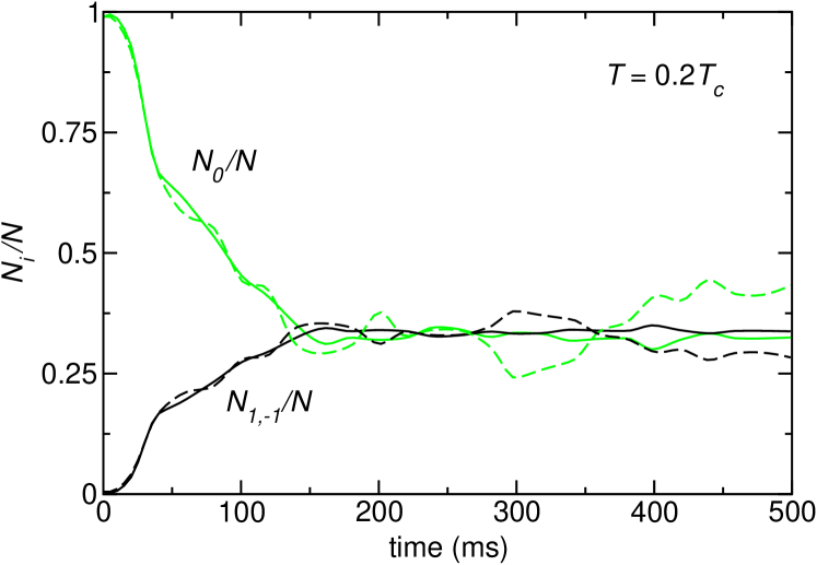
Figure 5.5: Population of the spin components as a function of time for the initial configuration $\bm{N}(t=0)/{\cal N}=(0.5\%,99\%,0.5\%)$ and $T=0.2T_{c}$. The labelling of the lines is as in Fig. 5.2.

In a spin-polarized, elongated condensate, the occurrence of phase fluctuations due to thermal excitations induces modulations of the density during an expansion of the system in a time scale of the order of 10 ms [KSS⁺03]. These density fluctuations are not expected inside the trap as the mean field prevents them, but in a time-of-flight experiment they can be used to quantify the phase fluctuations of the trapped system and also as a thermometry probe [KSS⁺03]. In a multicomponent condensate, one can follow the same argument to show that modulations of the total density should not be expected in the trap.

However, the situation is different for the densities of the various spin components. Indeed, the spin-exchange interaction ($\sim c_{2}n$) is much weaker than the scalar mean field ($\sim c_{0}n$), and it is not strong enough to prevent spin-density fluctuations, which lead to the formation of spin domains, cf. Fig. 5.6. This process is much faster at finite temperature than at $T=0$; for example, the number of spin domains at time $t=80$ ms for a temperature $T=0.2T_{c}$ is larger than at time $t=240$ ms for $T=0$. Such a fast domain formation has also been observed in simulations of pseudo-spin-1/2 systems [KT04]. This result contrasts with the relatively long times for the emergence of domains predicted by the theory and simulations of Zhang et al. [GaTe05b] and obtained in the simulations by Saito and Ueda [SU05b]. We think that this discrepancy may be due to the presence of the thermal clouds. Indeed, it has been argued that spin oscillations in the thermal cloud can considerably affect the spin dynamics in a finite-temperature condensate [JILA02] (see also [OL02]). With regards to this point, it is interesting to note that, even though our way of introducing thermal phase fluctuations does not take into account possible spin correlations among the clouds, the fact that the initial system is almost completely in one component may prevent such correlations from being relevant for the later dynamics.

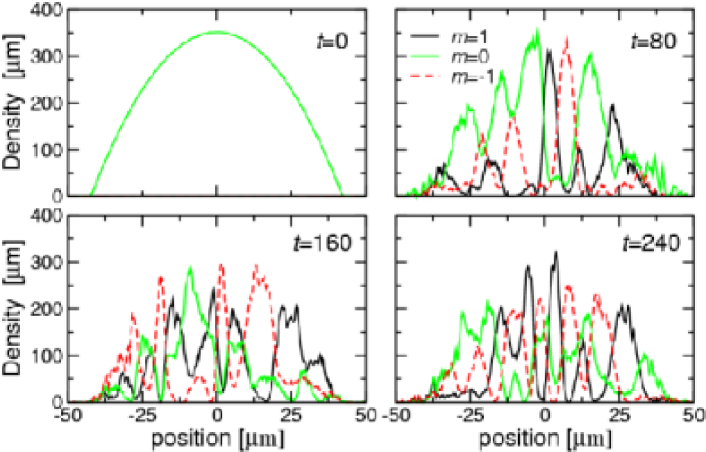
Figure 5.6: Density profiles of the spin components at different times (in ms) at $T=0.2T_{c}$ for the same initial configuration as before (dashed line in Fig.5.2). Again, the total density keeps the same profile throughout the simulation.

Moreover, the density profiles for the $m=\pm 1$ components at finite temperature are no longer equal as was the case at $T=0$. This is due to the existence of different thermal clouds for each component [JILA03b, Hamb04c, Hamb04a], which is accounted for in the simulation by having different random profiles for the corresponding thermal phases, $\theta^{\rm th}_{1}(z)\neq\theta^{\rm th}_{-1}(z)$. As a consequence, the local magnetization $n_{1}(z,t)-n_{-1}(z,t)$ is no longer constant as at $T=0$. Nevertheless, as expected, the total magnetization is still a conserved quantity along the time evolution.

The typical size of the domains $l_{\rm dom}$ can be estimated from our data to be $\sim$10 $\mu$m. Ueda [Ued01] and Saito and Ueda [SU05b] have studied the excitation modes of the system within a Bogoliubov-de Gennes scheme, and determined that it should undergo a dynamical instability through modes related to spin waves which carry angular momentum $\pm\hbar$. The most unstable modes according to them are those with a momentum $k_{\rm inst}$ that satisfies $2\pi/k_{\rm inst}\approx l_{\rm dom}$. Their simulations (for 1D and 2D systems) also present this typical domain size [SU05b]. They also note that this size should depend on the presence of a homogeneous magnetic field: for larger fields, the domain size would grow, reaching $\sim 16$ $\mu$m for $B=1$ G. This value is closer to the experimental results [GaTe05a] than ours. Also a recent work in an elongated 3D system by Zhang et al. [GaTe05b] reports a value similar to the experimental one including in the simulations a magnetic field $B=0.3$ G. Nevertheless, it is also possible that other thermal effects might be important. For example, spin excitation modes should be taken into account in our simulation on an equal footing to the phase fluctuations. To this end, the wave functions corresponding to the spectrum of spin excitations found in [Ho98, SU05b, GaTe05b] need to be calculated. Then, they should be thermally populated at the beginning of the simulation in a way similar to what we have done for the phase fluctuations.

Finally, we note that the results obtained by Saito and Ueda are for a system at zero temperature. The reason why they obtain a dynamical separation of the $\pm 1$ domains —contrary to our results, see Fig. 5.3— is that their starting input profiles have a small magnetization, which triggers the formation and development of spin waves along the system. Also, the dynamical instability appears in their calculations at later times $t\sim 300$ ms, even though they have more particles in the system, ${\cal N}=4\times 10^{6}$. These differences are most probably due to the fact that the inhomogeneity in the initial conditions that we impose through the phase fluctuations is more important, and favors the appearance of domains.

5.5.3 An ‘antiferromagnetic’ system: ${}^{87}\mbox{Rb}_{\mathrm{AF}}$

After studying the system of ⁸⁷Rb ($f=1$), that is ‘ferromagnetic’, we turn our attention to an ‘antiferromagnetic’ case, to check the prediction of Zhang et al. that for such systems no dynamical instabilities occur and, therefore, no domain formation is to be expected [GaTe05b]. A system naturally ‘antiferromagnetic’ is ²³Na in the $f=1$ hyperfine manifold. However, in order to do a direct comparison with the results of the previous section, we prefer to work in a model system, which is formed by ⁸⁷Rb atoms with $f=1$ but where we have changed the sign of the coupling constant $c_{2}$. In this way, only the spin dynamics is expected to change, while nothing different should happen to the total density as compared to the previous results. We will denote this artificial version of rubidium as ${}^{87}\mbox{Rb}_{\mathrm{AF}}$.

As before, we have performed simulations at zero and finite temperature. The results are presented in Figs. 5.7–5.8 and they are readily seen to be quite different from those corresponding to the ferromagnetic case. In figure 5.7 we present the evolution of the population of the different spin components at zero and finite temperature. The zero-temperature results, displayed by dashed lines, consist in almost perfect oscillations between the initial population $\bm{N}/{\cal N}=(0.5\%,99\%,0.5\%)$ and the exact mean-field ground state $(50\%,0\%,50\%)$ [ZYY03]. This behavior can be interpreted as Rabi-like oscillations of pairs of atoms between the states $|U\rangle$ and $|Z\rangle$, defined above [see discussion after Eq. (5.8)]. Indeed, the ground-state configuration is basically formed by ${\cal N}/2$ pairs in state $|U\rangle$ and the initial one has the same number of $|Z\rangle$ pairs; moreover, both states satisfy $|\langle\bm{F}\rangle|=0$ and are almost degenerate. However, the exchange of populations is not complete, and the overall data cannot be fitted by a simple sinusoidal function, but the oscillations seem to ‘speed up’ as time goes by: the two first maxima of $N_{0}/{\cal N}$ are separated $\approx 230$ ms, while the second and the third are $\approx 215$ ms apart. Again, this fact should be attributed to the nonlinearity of the sytem.

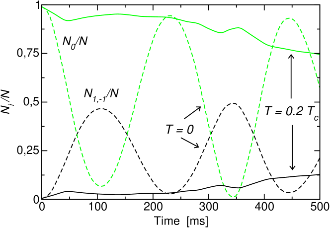
Figure 5.7: Population of the spin components as a function of time for the initial configuration $\bm{N}/{\cal N}=(0.5\%,99\%,0.5\%)$ and $\Theta=0$ for the ‘antiferromagnetic’ system ${}^{87}\mbox{Rb}_{\mathrm{AF}}$ (see text). The dashed lines are the results at $T=0$ while the solid lines have been calculated at $T=0.2T_{c}$.

The results for the simulation at $T=0.2T_{c}$ (solid lines) present a very different behavior. For the case $\Theta=0$, there is only a very slow decay of the population of the $m=0$ component, with the corresponding increase of the number of atoms in $m=\pm 1$. This is due in part to the fact that the chosen starting configuration is energetically very close to the ground state for the antiferromagnetic system, which will result in a long thermalization time. We also remark that in neither the zero-temperature or the finite-temperature cases a steady-state is observed in the simulated time of 500 ms, contrary to what happened for the ‘ferromagnetic’ case (cf. Figs. 5.2 and 5.5). One may expect, however, to converge to an equilibrium state with longer simulations.

The very slow evolution of the spin transfer in the finite-temperature case is also reflected in the density profiles, that we present in Fig. 5.8. Again, solid lines stand for the $T=0.2T_{c}$ case, while dashed lines are for the $T=0$ calculation, and the color coding is the same as in previous figures. At zero temperature, in the initial stages $t\lesssim 80$ ms, we see an evolution resembling that of the ‘ferromagnetic’ ⁸⁷Rb (compare Fig. 5.3). However, for $t=240$ ms the system practically turns back to its initial distribution, a behavior very different from the ‘ferromagnetic’ one, where one could observe the formation of spin domains. The differences are still more pronounced for the simulation at finite temperature, where there is essentially no evolution beyond some small fluctuations, coming from the random thermal phases. Only at very long times $t\sim 500$ ms (not shown in the figure for clarity) the $m=\pm 1$ clouds start to be visible on the scale of the figure.

Compared to the ‘ferromagnetic’ case in Fig. 5.6, one remarks the difficulty in forming separate spin domains, even though the thermal phases are different for all components. This must be attributed to the ‘antiferromagnetic’ character of the system under study, that tends to keep atoms in states $m=\pm 1$ together to minimize the local spin, $|\langle F\rangle|(z)=0$. On the other hand, one expects a separation of $m=\pm 1$ atoms from $m=0$ atoms, as observed experimentally for the case of ²³Na [MIT98b], which also explains the difficulty in populating the $m=\pm 1$ components starting from an almost pure 0-condensate.

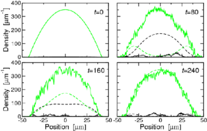
Figure 5.8: Density profiles for the ‘antiferromagnetic’ system ${}^{87}\mbox{Rb}_{\mathrm{AF}}$ for times $t=0$, 80, 160, 240 and 500 ms. The dashed lines are the results at $T=0$ while the solid lines have been calculated at $T=0.2T_{c}$. The initial configuration is $\bm{N}/{\cal N}=(0.5\%,99\%,0.5\%)$ with $\Theta=0$. The $m=0$ profile is plotted in green and the $m=1$ profile in black, while the red line in the last plot is for the $m=-1$ component.

5.6 Conclusions

In this chapter, we have studied the spin dynamics of a spin-1 ⁸⁷Rb condensate in a highly elongated trap, which we have modeled as a one-dimensional system. We have solved the three coupled dynamical equations for the spin components within a mean-field framework without any further approximations. This is in fact necessary, since approximated treatments, such as sma, frequently mask some of the aspects of the dynamics. We have also considered finite temperature effects. For one-dimensional systems at very low temperatures, these effects manifest themselves basically as phase fluctuations, which we have incorporated using the approach of Ref. [HDR⁺01] based on a thermo-statistical population of the excitations of the system.

We have found that the spin dynamics towards the steady state is not monotonic but rather slowly damped, involving a coherent exchange of population between the various spin components. At finite temperature, the coherent oscillations of populations among the $m=0$ and $m=\pm 1$ states are strongly damped. The internal coupling of the spin components together with the presence of a different thermal cloud for each component lead to the formation of numerous spin domains within the condensate. The size of these domains defines a characteristic length scale in the system, $l_{\rm dom}\sim 10\leavevmode\nobreak\ \mu$m, which does not decrease with time, and seems to be intrinsically determined by a dynamical instability of the excitation modes of the ‘ferromagnetic’ system, without noticeable thermal effects. Indeed, similar simulations for a system in which we have artificially changed the sign of the spin-exchange interaction present no formation of domains even at finite temperatures, as expected from theoretical considerations [GaTe05b].

For a ‘ferromagnetic’ condensate at zero temperature and with initially almost all atoms in the $m=0$ component and zero magnetization, the populations of the spin components oscillate around the configuration which corresponds to the ground state, $(25\%,50\%,25\%)$. On the other hand, at finite temperature the interaction of the condensate atoms with their thermal clouds leads to equipartition in populations $(1/3,1/3,1/3)$. However, recent simulations at zero temperature with a very small initial magnetization ${\cal M/N}=10^{-4}$ also drive the system to stationary states far from the ground state. Moreover, in these simulations formation of multiple spin domains is also observed. Therefore, the true role of thermal effects on the dynamics (beyond that of breaking the symmetry of the initial conditions of the $m=\pm 1$ components) is not clear yet, and deserves further consideration.

The results for an ‘antiferromagnetic’ case are very different. In particular, the dynamics of populations and density profiles is very slow, and no domains appear for times $t\lesssim 500$ ms starting from an almost-pure $m=0$ condensate. We have explained this result by the ‘antiferromagnetic’ character of the interactions in this system together with the quasi-degeneracy of the initial configuration with the mean-field ground state.

Our results might also be relevant to the question of decoherence. Our simulations, and in particular the finding of very fast domain formation, suggest that decoherence is enhanced as the number of components in the system is enlarged. Of course, there are many open questions connected to this, e. g., whether the formation of domains goes along with a loss of phase relations, and gives rise to some enhanced (generalized) phase fluctuations. It seems also interesting to study the mechanism underlying the speeding of domain formation by temperature. To this end, one might consider incorporating spin-density fluctuations already at the start of the simulation in a way similar to what has been done for the phase fluctuations.

Part II Two-dimensional helium systems

Motivation: helium as ‘the’ quantum liquid

In this second part of the thesis, we aim at studying a variety of helium systems, which are quite different from the ultracold, dilute gases. Helium has for a long time been considered ‘the’ quantum fluid, as many of its physical properties can be directly related to the quantum laws: from the fact that helium remains liquid down to zero temperature at saturation vapor pressure, to the superfluidity present in both the bosonic ⁴He and the fermionic ³He species. In fact, since the pioneering experiments of H. Kamerling Onnes to cool down helium and other substances [Kam11, Kam67], until the more recent claim for the observation of a supersolid phase in helium [KC04], the study of helium has received a lot of attention. This attention has rewarded us with a more profound understanding not only of this atomic species, but of the implications of quantum laws when applied to a many-body system.

Among the most striking experiments, one can mention: the liquefaction of helium by H. Kamerling Onnes (1908); the discovery of ⁴He superfluidity by Pyotr Kapitza [Kap37] and Allen and Misener [AM37]; the discovery of ³He superfluidity by Osheroff et al. [ORL72, OGRL72]. For later reference, we would also like to cite the production of helium clusters by supersonic expansion of a helium gas by Becker et al. [BKL61] –which finally led to the observation of the extremelly-weakly-bound helium dimer by Luo et al. [LMK⁺93], and by Sch llkopf and Toennies [ST94]– and the production of effectively low-dimensional helium systems by adsorbtion on a graphite by Bretz et al. [BDH⁺73].

A few theoretical works worth being cited as well are: the study of the role of the excitation spectrum in determining the superfluid behavior of ⁴He by Landau [Lan41, Lan47] and the introduction of correlations to account for the strong repulsion at short distances between two helium atoms by Jastrow [Jas55] and by Feynman [Fey54, FC56]. Finally, we would also like to emphasize the original application of density functional techniques to the study of atomic quantum liquids by Stringari [Str84, DS85].

Recently, a great deal of work has been devoted to study quantum liquids in restricted geometries [KN02]. One important feature of these systems is that their internal structure becomes more easily observable than in bulk liquids due to the restricted motion of the particles in the confining potential. Among these systems the study of quantum films has received particular attention. They consist of liquid helium adsorbed to a more-or-less attractive flat surface. In 1973, M. Bretz et al. [BDH⁺73] observed for the first time the adsorption of ⁴He onto the basal plane of graphite. In the last few years, adsorption properties of helium on different substrates such as carbon, alkali and alkaline-earth flat surfaces, carbon nanotubes and aerogels have become a fertile topic of research.

The structure and growth of thin films of ⁴He adsorbed to a substrate was studied by Clements et al. [CEKS93] employing the optimized hypernetted-chain Euler-Lagrange theory with realistic atom-atom interactions. It turns out that films with low surface coverages (where all atoms cover the surface with a thickness corresponding to a single atom), can be reasonably well described by a two-dimensional model. In connection with these systems, an interesting question naturally arises as how physics depends on the dimensionality of the space.

The homogeneous 2D liquid has been studied using different theoretical methods, such as molecular dynamics [CS71] and quantum Monte Carlo simulations, either Green’s Function [WCK88] or diffusion [GBC96a] techniques. The inhomogeneous case was studied by Krishnamachari and Chester who used a shadow variational wave function to describe 2D puddles of liquid ⁴He [KC99].

In the following two chapters we present our studies on ⁴He systems in two dimensions (2D). In Chapter 6 we report results of Variational (VMC) and Diffusion Monte Carlo (dmc) calculations. First, we introduce the Monte Carlo techniques. Then, we show our results for 2D clusters with a finite number of helium atoms. We study both the energetics and the density profiles of these systems.

In Chapter 7 we present a similar study developed in the framework of the Density Functional techniques, which allow us to study much larger clusters of ⁴He. We start the chapter giving a short introduction to theoretical background of our work: the Hohenberg-Kohn theorem and Density Functional theory. Then we present how to use the data obtained from the dmc calculations to set up a zero-range Density Functional. With this functional, we perform calculations for large clusters, which would be computationally prohibitive for a dmc calculation. Finally, we compare the results obtained with both methods.

Chapter 6 Quantum Monte Carlo study of two–dimensional ⁴He clusters

Your bait of falsehood takes this carp of truth:
And thus do we of wisdom and of reach,
With windlasses and with assays of bias,
By indirections find directions out.

William Shakespeare, Hamlet (II, 1)

6.1 Short introduction to Quantum Monte Carlo methods

Quantum Monte Carlo (qmc) methods are powerful numerical techniques to solve the Schr dinger equation for interacting many-body systems. There is a large variety of these methods: from the easy-to-program Variational Monte Carlo (vmc), to the more powerful Diffusion Monte Carlo (dmc) and Green’s Function Monte Carlo (gfmc) and the more sophisticated Path Integral Monte Carlo (pimc) that is able to cope with finite-temperature problems. One can find in the literature a number of introductions to and comparisons among the various methods, see e. g. [Cep95, Gua98, HLR94] and also [Ast04, Wil96]. Here we will just present a concise introduction to the philosophy and algorithms actually used in our calculations (vmc and dmc).

6.1.1 Importance sampling and Metropolis algorithm

Let us denote by $\Phi$ a wave function corresponding to some state of our interacting system. The postulates of Quantum Mechanics say that

$$p(\bm{R})=\frac{|\Phi(\bm{R},t)|^{2}}{\int\mathrm{d}\bm{R}\,|\Phi(\bm{R},t)|^{2}}\mathrm{d}\bm{R}\;,$$ (6.1)

with $\bm{R}=\{\bm{r}_{1},\bm{r}_{2},\cdots,\bm{r}_{N}\}$, is the probability that the $N$ particles of the system (in our case, ⁴He atoms in a droplet) are located within a volum $\mathrm{d}\bm{R}$ around the positions $\{\bm{r}_{1},\bm{r}_{2},\cdots,\bm{r}_{N}\}$, at time $t$ [GP89, Mes99]. Indeed, $\Phi$ contains all the information that could in principle be retrieved from the system.

However, we are usually interested only on averages of operators weighed with $p(\bm{R})$,

$$\langle\hat{A}\rangle=\frac{\langle\Phi|\hat{A}|\Phi\rangle}{\langle\Phi|\Phi\rangle}=\int\mathrm{d}\bm{R}\,p(\bm{R})A(\bm{R})\>.$$

For example, the energy of a state is just the expectation value of the Hamiltonian in such a state:

$$E[\Phi] =\frac{\langle\Phi|\hat{H}|\Phi\rangle}{\langle\Phi|\Phi\rangle}=T+V=$$

$$\!\!\!\!=\frac{\sum_{i=1}^{N}\int\mathrm{d}\bm{R}\,\Phi^{*}(\bm{R})\frac{-\hbar^{2}\nabla_{i}^{2}}{2m}\Phi(\bm{R})}{\int\mathrm{d}\bm{R}\,|\Phi(\bm{R})|^{2}}+\frac{\sum_{i<j}\int\mathrm{d}\bm{R}\,{\hat{V}}(\bm{r}_{i},\bm{r}_{j})|\Phi(\bm{R})|^{2}}{\int\mathrm{d}\bm{R}\,|\Phi(\bm{R})|^{2}}\;,$$ (6.2)

where we assumed that only two-body interactions $\hat{V}$ are present. In order to know $E[\Phi]$ not all the information contained in $\Phi$ is required, but just some information on its spatial variations (to evaluate the kinetic energy $T$) and the two-point distribution function obtained once the coordinates of $N-2$ particles have been integrated out. Therefore, two questions must be addressed: (1) how to find a good approximation to the wave function $\Phi$ of interest (usually, the ground-state wave function); and (2) how to calculate these averages once the wave function is given.

One could naïvely think in a $\mathbb{R}^{Nd}$-generalization of the simple trapezoidal approximation with $M$ points to a one-dimensional integral,

$$\int_{a}^{b}\mathrm{d}x\,f(x)\approx\frac{b-a}{M}\sum_{k=1}^{M}f(x_{k})\,,\qquad x_{k}=a+\frac{k}{M}(b-a)\,$$

the main difference being that now the integration is over $Nd$ dimensions. However, the exponential increase in size of the (hyper)volume of integration with the number of particles in the system, together with the fact that most of this (hyper)space usually contributes poorly to the total value of the integral, make such ‘traditional’ integration rules (trapezoidal, Simpson’s, orthogonal polynomials, etc.) unapplicable, and one has to resort to more sophisticated methods such as Monte Carlo techniques.

Here one evaluates averages such as those in (6.2) stochastically: a number $N_{W}$ of points (called walkers) $\{\bm{R}_{k}\}\leavevmode\nobreak\ (k=1,\cdots,N_{W})$ are randomly drawn in $\mathbb{R}^{Nd}$ according to the probability distribution $p(\bm{R})$. Therefore, more points are generated where they have more weight, and very few (if any) where the contribution to the integral is small. The fact that the points are sorted according to $|\Phi|^{2}$ is what makes these quadrature techniques so powerful to perform multi-dimensional integrations. One usually refers to the function used to weigh the configurations (in the present case, $\Phi$) as the ‘importance function’, and the technique ‘importance sampling’.

Then, the values of the energy of the system (or whatever the observable to estimate is) in such configurations $e_{k}=e(\bm{R}_{k})$ are recorded. For a large enough number of points $\bm{R}_{k}$, the Central Limit theorem guarantees that

$$E[\Phi]=\int\mathrm{d}\bm{R}\,e(\bm{R})p(\bm{R})=\frac{1}{N_{W}}\sum_{k}e_{k}\>.$$ (6.3)

One way to obtain a set of points in $\mathbb{R}^{Nd}$ distributed according to $p(\bm{R})$ is by means of the Metropolis algorithm [MRR⁺53]:

1. Start by generating $N$ positions $\{\bm{r}_{i}\}\leavevmode\nobreak\ (i=1,\cdots,N$) distributed randomly within configuration space. These points define an starting walker, $\bm{R}$.

2. For each position, perform a random move as

   $$\bm{r}^{\prime}_{i}=\bm{r}_{i}+\ell\bm{\xi}_{i}\,,$$

   where $\ell$ is the typical size of the random step, and $\bm{\xi}_{i}$ is a three-component vector whose elements are random numbers uniformly distributed in $[-\tfrac{1}{2},\tfrac{1}{2}]$. Thus, each particle in the walker has moved from its original position to a new one inside a box of side $\ell$ around it.

3. The probabilities of the system being in the configuration corresponding to $\bm{R}=\{\bm{r}_{1},\cdots,\bm{r}_{N}\}$ and its proposed successor $\bm{R}^{\prime}=\{\bm{r}^{\prime}_{1},\cdots,\bm{r}^{\prime}_{N}\}$ are calculated. Then, the proposed movement $\bm{R}\rightarrow\bm{R}^{\prime}$ is accepted with a probability:

   $$P(\bm{R}\rightarrow\bm{R}^{\prime})=\begin{cases}1&p(\bm{R}^{\prime})\geq p(\bm{R})\\ p(\bm{R}^{\prime})/p(\bm{R})&p(\bm{R}^{\prime})<p(\bm{R})\\ \end{cases}\>,$$

   If the movement is accepted, we set $\bm{r}_{i}=\bm{r}^{\prime}_{i}\leavevmode\nobreak\ \forall i$. Otherwise, we keep $\bm{R}$ as is; that is, the new walker is identical to its predecessor.

4. After a certain number of iterations of steps 2–3 (‘equilibration loop’), the set of points in the last walker should be distributed according to $p(\bm{R})$. Then, it is time to start saving data to perform the average of Eq. (6.3). To this end, one performs again a number of iterations of steps 2–3, but now the quantity to be averaged is stored with the value corresponding to $\bm{R}$ after the acceptance/rejection step (‘averaging loop’). That is, if the new walker is identical to its predecessor, one must record the same value $e(\bm{R})$ saved in the previous loop.

A chart illustrating this process is in Fig. 6.1. The size of the step $\ell$ must be chosen carefully: too short a step will result in a large acceptance of moves, but also in very correlated configurations and a long time to reach equilibrium. On the other hand, too long a step will probably result in a large number of rejected moves, and also a long time for equilibration. A good choice is the one that results in an acceptance around $50\%-70\%$ [Gua98]. In our calculations, $\ell\approx 6$ Å.

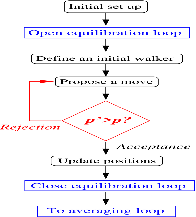
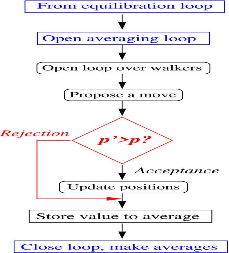
Figure 6.1: Flow chart of the Metropolis algorithm: equilibration process (left) and averaging process (right).

It is also important to note that both the equilibration and averaging loops have to be repeated a number of times, called blocks. Indeed, each configuration produced in a step of the Metropolis algorithm is strongly correlated with the previous one. Thus, a direct average as suggested in (6.3) would produce typically too small a variance. In order to have uncorrelated data $e_{k}$ to average, one divides the simulation in a set of blocks, each of which composed of a certain number of simulation steps. For each block, an average of the energies accumulated in it is performed, resulting in a ‘block estimate’ for the the energy $e_{\rm block}$. A careful analysis on the length of the blocks has to be performed in order to ensure that the configurations in the different blocks are uncorrelated, so that the $e_{\rm block}$ values are effectively independent (see [FP89, Nig98]). Once this has been done, one can finally give an estimate for the energy and the associated uncertainty,

$$\bar{e} =\frac{1}{N_{\rm blocks}}\sum_{\rm block=1}^{N_{\rm blocks}}e_{\rm block}$$

$$\Delta e =\sqrt{\frac{1}{N_{\rm blocks}-1}\sum_{\rm block=1}^{N_{\rm blocks}}\left(e_{\rm block}-\bar{e}\right)^{2}}\>,$$

where $N_{\rm blocks}$ is the number of blocks in the averaging loop. In our simulations, typically $N_{\rm blocks}\approx 100$, and the number of Monte Carlo steps per block $N_{\rm steps}\approx 1000$.

6.1.2 Variational Monte Carlo

The Variational Monte Carlo (vmc) method relies on the ‘Variational Theorem’, which can be stated in this way:

Variational theorem.

The expectation value of the Hamiltonian over an arbitrary wave function $\Phi$ is larger than, or equal to, its expectation value on the exact ground state, $E_{0}$. The equality only holds if $\Phi$ coincides with the exact ground state wave function, $\Psi_{0}$.

Proof.

This theorem is easily proved expanding $\Phi$ on the basis of eigenstates of the Hamiltonian $\{\Psi_{n}\}\leavevmode\nobreak\ (n=0,1,2,\cdots)$ (with corresponding eigenenergies $\{E_{n}\}$). Without loss of generality, we assume that $\Phi$ is already normalized to unity, so that we can write

$$|\Phi\rangle =\sum_{n}c_{n}|\Psi_{n}\rangle\,,$$

$$c_{n} :=\langle\Psi_{n}|\Phi\rangle\,,\qquad|c_{n}|\in[0,1]\,,\quad\sum_{n}|c_{n}|^{2}=1\>.$$

Now, we insert this expression into the expectation value of the Hamiltonian:

$$\langle\Phi|\hat{H}|\Phi\rangle =\sum_{nm}c_{n}^{*}c_{m}\langle\Psi_{n}^{*}|H|\Psi_{m}\rangle=\sum_{nm}c_{n}^{*}c_{m}\langle\Psi_{n}^{*}|E_{m}|\Psi_{m}\rangle=$$

$$=\sum_{nm}c_{n}^{*}c_{m}E_{m}\delta_{nm}=\sum_{n}|c_{n}|^{2}E_{n}\geq E_{0}\>,$$

where we assumed that the eigenstates are properly orthonormalized and ordered in such a way that $E_{0}\leq E_{1}\leq\cdots$. ∎

In a vmc calculation, one proposes a trial wave function $\Phi_{T}$ with one or more (say $p$) variational parameters $\{\alpha_{i}\}\leavevmode\nobreak\ (i=1,\cdots,p)$. The functional form assumed should be based on all the available physical information of the system, and not too many variational parameters should be included in order to simplify the minimization process. The scope is to find the values of the parameters $\{\overline{\alpha}_{i}\}$ that minimize the expectation value

$$E_{T}(\{\alpha_{i}\}):=E[\Phi_{T}]=\frac{\langle\Phi_{T}|\hat{H}|\Phi_{T}\rangle}{\langle\Phi_{T}|\Phi_{T}\rangle}\>.$$ (6.4)

The corresponding wave function $\Phi(\{\overline{\alpha}_{i}\})$ will be the best approximation to $\Psi_{0}$ with the functional form of $\Phi$.

One evaluates the expectation value $E[\Phi_{T}]$ stochastically as outlined above. For the case of two-body interactions, and taking for simplicity a central interparticle potential, $V(\bm{r}_{i},\bm{r}_{j})=V(|\bm{r}_{i}-\bm{r}_{j}|)$, we have

$$e(\bm{R})=-\sum_{i=1}^{N}\frac{\hbar^{2}}{2m}\frac{\nabla_{i}^{2}\Phi_{T}(\bm{R})}{\Phi_{T}(\bm{R})}+\sum_{i<j}V(|\bm{r}_{i}-\bm{r}_{j}|)\>.$$ (6.5)

Note that this expression is only meaningful for $\Phi_{T}(\bm{R})\neq 0$. This is not a problem since configurations for which $\Phi_{T}(\bm{R})=0$ are in fact discarded by the Metropolis algorithm. There will be no problems in implementing this algorithm for Bose sytems, whose ground states are known to have no zeroes [MPM02]. The situation is more complex for fermionic systems, where Pauli’s principle forces $\Psi(\bm{R})$ to vanish whenever $\bm{R}$ contains two indistinguishable particles in the same position, e. g. $\Phi(\bm{r}_{1},\cdots,\bm{r},\cdots,\bm{r},\cdots,\bm{r}_{N})\equiv 0$. This is known as the ‘sign problem’ for fermionic systems, and a number of methods have been developed to overcome it. However, as we are interested in the study of ⁴He, which is bosonic and will not suffer this problem, we will not discuss further this point, but refer the reader to the literature [Cep98, HLR94, Wil96, Ast04].

A good feature of vmc calculations is the ‘control’ on the wave function that one has. Indeed, the calculated value (6.4) will depend on the functional form of $\Phi_{T}$ and the values of its variational parameters $\alpha_{i}$. Therefore, one can get insight into the physics of the problem by checking different forms for $\Phi_{T}$, which parameters affect more the value of $E_{T}$ and, finally, what are the optimal values for these parameters.

Also, if one has been able to find the exact ground-state wave function, $\Psi_{0}$, one can make averages as that in Eq. (6.2) for any operator in order to retrieve more information on the system, which might be too difficult to extract analytically. For example, the exact ground state of a one-dimensional system of hard-core bosons is known to be the absolute value of a Slater determinant of plane waves. In this case, despite having the exact $\Psi_{0}$, analytical calculations are quite difficult, and Monte Carlo methods have been useful to obtain its momentum distribution, correlation functions, etc. [Ast04].

As a drawback, vmc is unable to correct by itself any ‘bad’ behavior (symmetries, long- or short- range orders, etc.) that we may have introduced in $\Phi$. That is, if we have assumed a wave function with a different symmetry than $\Psi_{0}$, the vmc calculation will be equally valid, but the upper bound we obtain for the ground state energy may be far from its true value. Any other expectation value that we calculate will be equally biased. A way to overcome these problems is to perform a Diffusion Monte Carlo, calculation which is able to provide the exact ground state energy for a Bose system.

6.1.3 Diffusion Monte Carlo

The Diffusion Monte Carlo (dmc) method consists of a stochastic solution of the Schr dinger equation,

$$i\hbar\frac{\partial}{\partial t}\Phi(\bm{R},t)=\hat{H}\Phi(\bm{R},t)\>.$$

We introduce an ‘imaginary time’ variable $\tau=it$, so that

$$-\hbar\frac{\partial}{\partial\tau}\Phi(\bm{R},\tau)=(\hat{H}-E_{T})\Phi(\bm{R},\tau)\>,$$ (6.6)

being $E_{T}$ an (arbitrary) energy shift whose utility will become clear below. The formal time-dependent solution to this equation can be easily expressed in terms of the eigenfunctions and eigenenergies of the Hamiltonian as

$$\Phi(\bm{R},\tau)=\sum_{n=0}^{\infty}c_{n}\Psi_{n}(\bm{R},\tau)=\sum_{n}c_{n}e^{-(\hat{H}-E_{T})\tau/\hbar}\Psi_{n}(\bm{R},0)\\ =\sum_{n}c_{n}e^{-(E_{n}-E_{T})\tau/\hbar}\Psi_{n}(\bm{R},0)\stackrel{{\scriptstyle\tau\rightarrow\infty}}{{\longrightarrow}}c_{0}\Psi_{0}(\bm{R},0)e^{-(E_{0}-E_{T})\tau/\hbar}\>.$$

Therefore, a trial function propagated on imaginary time, will converge to the ground state of the system, as long as it is not orthogonal to it ($c_{0}\neq 0$). In general, the propagation will converge to the less energetic state with a non-vanishing overlap with $\Phi$, while the other components are exponentially suppressed. Moreover, if the energy shift $E_{T}$ equals the ground-state energy $E_{0}$, $\Phi(\bm{R},\tau)$ has a stationary behavior at large $\tau$, which coincides with the ground state solution (up to a normalization constant).

Let us see now how to perform this propagation on imaginary time. To this end, we consider a Hamiltonian with two-particle interactions $V$ and a possible external potential $V_{\rm ext}$,

$$\hat{H}=-\frac{\hbar^{2}}{2m}\sum_{i=1}^{N}\nabla_{i}^{2}+\sum_{i=1}^{N}V_{\rm ext}(\bm{r}_{i})+\sum_{i<j}V(r_{ij})$$

where $r_{ij}:=|\bm{r}_{i}-\bm{r}_{j}|$. The Schr dinger equation in imaginary time for this Hamiltonian can be cast in the form

$$-\hbar\frac{\partial}{\partial\tau}\Phi(\bm{R},t)=-D\nabla_{\bm{R}}^{2}\Phi+V(\bm{R})\Phi-E_{T}\Phi\>,$$ (6.7)

where we defined $D=\hbar^{2}/(2m)$ and $V(\bm{R})=\sum_{i}V_{\rm ext}(\bm{r}_{i})+\sum_{i<j}V(r_{ij})$, and $\nabla_{\bm{R}}^{2}$ is a shorthand notation for $\sum_{i}\nabla_{i}^{2}$. Next, we define a function $f$ as the product of the exact ground-state wave function, $\Psi$, and a trial one

$$f(\bm{R},\tau):=\Phi_{T}(\bm{R})\Psi(\bm{R},\tau)\>.$$

One can optimize the convergence of the dmc procedure by starting from a ‘reasonable’ trial function, typically obtained in a previous vmc calculation. Substitution of this expression into (6.7) gives an equation for $f$ that is fully equivalent to the Schr dinger equation,

$$-\hbar\frac{\partial}{\partial\tau}f=-D\nabla_{\bm{R}}^{2}f+D\bm{\nabla}_{\bm{R}}\cdot\left[\bm{F}f\right]+(E_{\rm loc}-E_{T})f\>,$$ (6.8)

with the definitions

$$\bm{F} :=\frac{2}{\Phi_{T}}\bm{\nabla}_{\bm{R}}\Phi_{T}$$ quantum drift force, (6.9a)

$$E_{\rm loc} :=\frac{1}{\Phi_{T}}\hat{H}\Phi_{T}$$ local energy. (6.9b)

The use of $f$ instead of $\Psi$ is recommended because it reduces the variance of the calculated observables.

The formal solution of Eq. (6.8) in $\bm{R}$-space can be written as

$$f(\bm{R},\tau)\equiv\langle\bm{R}|f(\tau)\rangle=\int\mathrm{d}\bm{R}\,^{\prime}\langle\bm{R}|e^{-(\hat{H}-E_{T})\tau/\hbar}|\bm{R}^{\prime}\rangle\langle\bm{R}^{\prime}|f(0)\rangle\equiv\\ \equiv\int\mathrm{d}\bm{R}\,^{\prime}G(\bm{R},\bm{R}^{\prime},\tau)f(\bm{R}^{\prime},0)\>,$$ (6.10)

where we have introduced the Green’s function

$$G(\bm{R},\bm{R}^{\prime},\tau):=\langle\bm{R}|e^{-(\hat{H}-E_{T})\tau/\hbar}|\bm{R}^{\prime}\rangle\>.$$

Up to this point, no approximations have been made, which means that if we were able to know the exact $G$, we could get $f(\bm{R},\tau)$ for any $\tau$ and obtain from it the ground state wave function $\Psi$. However, usually one does not know $G$ exactly, but it can only be found for small time steps. Then, the value of $f(\bm{R},\tau)$ for $\tau\rightarrow\infty$ is found iteratively,

$$f(\bm{R},\tau+\delta\tau)=\int\mathrm{d}\bm{R}\,^{\prime}G(\bm{R},\bm{R}^{\prime},\delta\tau)f(\bm{R}^{\prime},\tau)\>.$$

To obtain a reasonable approximation for $G$, let us split the operator acting of $f$ in Eq. (6.8) into three parts as follows

$$\hat{H}_{1} =-D\nabla_{\bm{R}}^{2}$$ (6.11a)

$$\hat{H}_{2} =D\left[\left(\bm{\nabla}_{\bm{R}}\cdot\bm{F}\right)+\bm{F}\cdot\bm{\nabla}_{\bm{R}}\right]$$ (6.11b)

$$\hat{H}_{3} =E_{\rm loc}(\bm{R})-E_{T}\>.$$ (6.11c)

We define also the Green’s functions characteristic of these operators:

$$G_{i}(\bm{R},\bm{R}^{\prime},\tau):=\langle\bm{R}|e^{-\hat{H}_{i}\tau/\hbar}|\bm{R}^{\prime}\rangle\>.$$

Even though the operators $\hat{H}_{i}$ do not commute with each other, we can use the Baker-Campbell-Hausdorff formula [Cam98, Bak02, Hau06, Wil67, Ryd96],

$$\exp{\hat{X}}\exp{\hat{Y}}=\exp\left(\hat{X}+\hat{Y}+\tfrac{1}{2}[\hat{X},\hat{Y}]+\cdots\right)\>,$$ (6.12)

to approximate the exponential to some fixed order for short time lapses $\delta\tau$; for example, to first order, we have

$$e^{-(\hat{H}-E_{T})\delta\tau/\hbar}=e^{-\hat{H}_{1}\delta\tau/\hbar}e^{-\hat{H}_{2}\delta\tau/\hbar}e^{-\hat{H}_{3}\delta\tau/\hbar}+O(\delta\tau^{2})$$ (6.13)

Similar expressions can be built with a higher degree of accuracy (i. e., valid up to a higher power of $\delta\tau$). Then, the full Green’s function will read

$$G(\bm{R},\bm{R}^{\prime},\tau)=\iint\mathrm{d}\bm{R}_{1}\mathrm{d}\bm{R}_{2}\,G_{1}(\bm{R},\bm{R}_{1},\tau)G_{2}(\bm{R}_{1},\bm{R}_{2},\tau)G_{3}(\bm{R}_{2},\bm{R}^{\prime},\tau)\>.$$

The solutions for the separate Green’s functions are easy to find. For example, $\hat{H}_{1}$ corresponds to a purely diffusive problem, and the solution is well-know to be that of a random walk

$$G_{1}(\bm{R},\bm{R}^{\prime},\tau)=\left(4\pi D\tau\right)^{-3N/2}\exp\left[-\frac{\left(\bm{R}-\bm{R}^{\prime}\right)^{2}}{4D\tau}\right]\>.$$

The effect of $\hat{H}_{2}$ is the same as that of a classical drift force $\bm{F}$ pointing towards the regions where the trial wave function is maximal:

$$G_{2}(\bm{R},\bm{R}^{\prime},\tau) =\delta\left(\bm{R}-\bm{R}(\tau)\right)\>,$$

$$\bm{R}(\tau) \text{ such that }\left\{\begin{array}[]{l}\bm{R}(0)=\bm{R}^{\prime}\\ \frac{\partial\bm{R}}{\partial\tau}=D\bm{F}\!\left(\bm{R}(\tau)\right)\end{array}\right.\>.$$

Finally, the Green’s function corresponding to $\hat{H}_{3}$ is

$$G_{3}(\bm{R},\bm{R}^{\prime},\tau)=\exp[(E_{T}-E_{\rm loc}(\bm{R}))\tau/\hbar]\delta\left(\bm{R}-\bm{R}^{\prime}\right)\>.\\$$

The effect of $G_{1}$ and $G_{2}$ is implemented by proposing random movements of walkers of the type

$$\bm{R}_{i}\rightarrow\bm{R}^{\prime}_{i}=\bm{R}_{i}+\bm{\xi}_{i}+\frac{\hbar^{2}t}{m}\bm{F}\>,$$

where $\bm{\xi}_{i}$ is a $3N$-component vector whose elements are random numbers generated according to a $Normal(0,1)$ distribution. The $G_{3}$ term is usually called the ‘branching term’ as it is the only contribution to $G$ that does not conserve the weights of the walkers as provided by $\Phi_{T}$: walkers with lower $E_{\rm loc}$ adquire larger weights, while those with larger $E_{\rm loc}$ have smaller weights. This is implemented in the algorithm in the following way:

1. The factor $s=\exp[(E_{T}-E_{\rm loc}(\bm{R}))\tau/\hbar]$ is computed for each walker.

2. A number $\xi$ is randomly generated with uniform distribution in [0,1].

3. The integer part of $n_{\rm sons}=s+\xi$ is calculated.

4. The walker $\bm{R}$ is replicated $n_{\rm sons}$ times. (In practice, we set a maximum value $n_{\rm sons}=10$ in our calculations.)

Thus, walkers with lower $E_{\rm loc}$ ‘reproduce’, while those with larger $E_{\rm loc}$ ‘die out’. This behavior will ultimately correct any component of the assumed $\Phi_{T}$ orthogonal to $\Psi$. Note that if $\Phi_{T}$ happens to be an eigenstate of $\hat{H}$, $E_{\rm loc}(\bm{R})\equiv E_{\rm loc}$ [cf. Eq. (6.9b)]: all walkers have the same weight and no ‘reproduction effects’ take place. In the chart of Fig. 6.1, this process takes place after updating the positions and before storing the values for the averages.

6.1.4 Building the trial function

From the previous discussion, we see that a crucial ingredient in both vmc and dmc calculations is the definition of the trial wave function $\Phi_{T}$. Indeed, the ‘velocity’ to converge from a given $\Phi_{T}$ to the exact ground state wave function will depend on the ‘distance’ between these two functions, and the accuracy of the average values obtained with the converged $f$ will also depend on it. Therefore, we must construct $\Phi_{T}$ carefully.

For a Hamiltonian with central, two-body interactions, even if they are strong as in the case of helium, experience has shown that a good guess has the Jastrow form [Jas55, PM02]

$$\Phi_{T}={\cal N}\left[\prod_{i=1}^{N}f_{1}(\bm{r}_{i})\right]\left[\prod_{j<k}f_{2}(r_{jk})\right]\>.$$ (6.14)

Here $\cal N$ is the normalization constant and $f_{1}$ is a one-body function accounting for the effects of a possible external potential. In our case of two-dimensional droplets, we simulate the self-trapping of the systems by introducing single-particle factors of the forms

$$f_{1}(r) =\exp\left[-\frac{\alpha^{2}}{2}r^{2}\right]$$ harmonic; (6.15a)

$$f_{1}(r) =\exp\left[-{\alpha}r\right] \text{exponential}.$$ (6.15b)

As it will be shown later, however, only the translationally invariant part of $\prod f_{1}$ is to be used as there is no external trapping potential that locates the droplet in space.

On the other hand, $f_{2}$ contains two-body correlations and should go to unity for large inter-particle distances. In particular, for studies on liquid helium the following form introduced by McMillan [McM65] has shown to be useful:

$$f_{2}(r)=\exp\left[-\frac{1}{2}\left(\frac{b}{r}\right)^{\nu}\right]\>.$$ (6.16)

Here $b$ and $\nu$ act as variational parameters with respect to which the expectation value $\langle\Phi_{T}|\hat{H}|\Phi_{T}\rangle$ will be minimized. For helium in three dimensions, the values $b\approx 3$ Å and $\nu\approx 5$ provide a good Ansatz for the calculations, as they account for the strong repulsion at short distances $r\lesssim\sigma=2.556$ Å characteristic of the helium-helium interaction, which in our calculations is described by the Aziz HFD-B(HE) potential [AMW87], see Fig. 6.2. As these values are related basically to the two-body potential, we think they will also be a reasonable starting point for our two-dimensional case. We note that these values give the correct behavior of the correlation function at short distances but they do not produce the correct behavior at long distances. However, we expect this not to be so important for finite systems such as the small droplets we will be dealing with [PPW86].

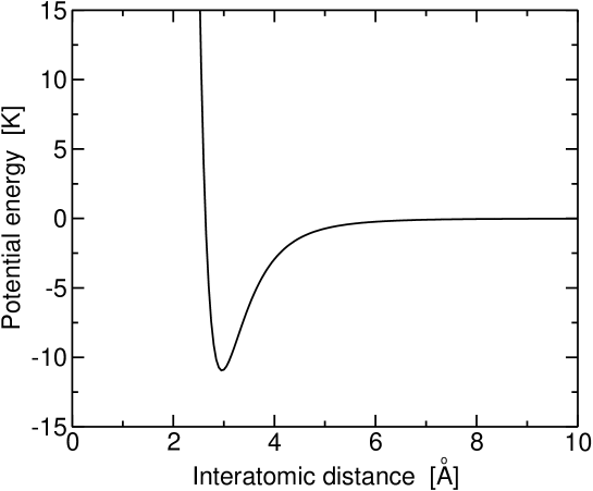
Figure 6.2: Aziz HFD-B(HE) interaction potential for ⁴He atoms.

6.2 vmc ground-state energies

To study a system of $N$ ⁴He atoms in two dimensions we start from the following trial wave function

$$\Phi_{T}({\bf R})=\prod_{i<j}\exp\left[-\frac{1}{2}\left(\frac{b}{r_{ij}}\right)^{\nu}-\frac{\alpha^{2}}{2N}r^{2}_{ij}\right]\,.$$ (6.17)

The first term inside the brackets corresponds to the simple McMillan two-body correlation, while the second term is the translationally invariant part of a harmonic oscillator (ho) wave function with parameter $\alpha$, extracted from the relation

$$\sum_{i=1}^{N}r_{i}^{2}=\frac{1}{N}\sum_{i<j}r_{ij}^{2}+\frac{1}{N}R_{\rm CM}^{2}\>,$$

to roughly confine the system to a region of radius $\sim\alpha^{-1}$.

In our calculations, we employ the value $\hbar^{2}/m_{4}=12.1194$ K Å² for the atom mass. The parameters $b$ and $\nu$ have been fixed to the values 3.00 Å and 5, respectively thus restricting the variational search to the ho parameter $\alpha$. The optimal values found as a function of the number of particles in the droplet are given in Table 6.1 together with the expectation value of the Hamiltonian and the separate contributions of kinetic and potential energies. It can be seen that the total energy results from an important cancellation between these contributions, which is in fact larger than in the 3D case. Let us recall that in 3D bulk, the energy per particle results from adding $\approx$ 14 K of kinetic energy to $\approx-21$ K of potential energy. In 2D, both kinetic and potential contributions are very similar, hence calculations are more delicate owing to the statistical uncertainties.

Table 6.1: Variational results for the ground-state energy per particle $E/N$ of 2D ⁴He puddles of various cluster sizes. The optimal confining ho parameter $\alpha$ is given in Å^-1 and all energies are in K. The expectation values of the kinetic and the potential energies are also displayed. The column labelled KC refers to the vmc results of Ref. [KC99]. The numbers in parenthesis stand for the statistical uncertainty on the last figure.

$N$	$\alpha$	$E/N$	$T/N$	$V/N$	KC
$8$	$\leavevmode\nobreak\ 0.1565$	$-0.2239(2)$	$1.3003(6)$	$-1.5242(5)$	—
$16$	$\leavevmode\nobreak\ 0.129$	$-0.3510(2)$	$1.7354(6)$	$-2.0864(5)$	$-0.380(8)$
$36$	$\leavevmode\nobreak\ 0.094$	$-0.4532(4)$	$2.031(3)$	$-2.484(3)$	$-0.471(7)$
$64$	$\leavevmode\nobreak\ 0.073$	$-0.4961(7)$	$2.159(2)$	$-2.655(2)$	$-0.528(5)$
$121$	$\leavevmode\nobreak\ 0.054$	$-0.5241(6)$	$2.223(2)$	$-2.747(2)$	$-0.570(7)$
$165$	$\leavevmode\nobreak\ 0.047$	$-0.5328(3)$	$2.289(1)$	$-2.822(1)$	$-0.602(7)$
$512$	$\leavevmode\nobreak\ 0.0266$	$-0.5493(5)$	$2.282(3)$	$-2.831(3)$	$-0.621(2)$
$\infty$	$\leavevmode\nobreak\ 0.0000$	$-0.6904(8)$	$4.312(2)$	$-5.003(1)$	—

The last column of Table 6.1 reports the vmc results of Krishnamachari and Chester [KC99]. As compared with their results, our calculations provide smaller binding energies in spite of the fact that the interaction used in [KC99] is an older version of the Aziz potential, which tends to underbind the systems. This is due to their use of shadow wave functions, which contain more elaborate correlations not present in our simple trial wave function. Finally, the vmc energy for the bulk system corresponds to the saturation density obtained in the dmc calculation of Ref. [GBC96a], $\rho_{0}=0.04344$ Å^-2.

We have also performed calculations using a different trial wave function, replacing the translationally invariant ho part by an exponential one, i. e.

$$\Phi_{T}({\bf R})=\prod_{i<j}\exp\left[-\frac{1}{2}\left(\frac{b}{r_{ij}}\right)^{\nu}-\frac{\alpha}{2}r_{ij}\right],$$ (6.18)

to check whether a larger tail in the wave function results in more binding. Actually, we do not find significant differences for small values of $N$. For instance, in the case $N=8$, using the same values for $b$ and $\nu$ as before, we get $E/N=-0.2178(5)$ K, $T/N=1.266(2)$ K, $V/N=-1.484(2)$ K for $\alpha=0.035$ Å^-1. When the values of $b$, $\nu$ and $\alpha$ are all optimized, we obtain a slightly larger binding energy, $E/N=-0.2267(8)$ K for $b=3.04$ Å, $\nu=5.0$ and $\alpha=0.035$ Å^-1. For greater values of $N$, the harmonic Ansatz tends to provide more binding than the exponential. For example, with the exponential Ansatz, for $N=16$ we get $E/N=-0.1816(7)$ K for $\alpha=0.023$ Å^-1, and optimizing the different parameters we get $E/N=-0.2514(6)$ K, with $b=3.04$ Å. In conclusion, the correlated ho wave function (6.17) seems good enough to be used as importance function in the dmc calculations.

6.3 dmc ground-state energies

After finding appropriate trial wave functions $\Phi_{T}(\alpha)$ with the previous vmc calculation, we will now perform dmc calculations to find the exact ground state energy and density profiles of the ⁴He two-dimensional clusters. We have used both first and second order [BC94] propagators [see Eq. (6.13)] in the present work and both of them provide the same extrapolated energy, within statistical uncertainties, using the optimal trial function of the vmc calculation as guiding function.

Our simulations have been carried out with a population of typically 400 walkers. As usual, some ‘equilibration’ runs are first done to establish the asymptotic region of the short time propagator. Then the average blocks are performed. This procedure is done for several values of the time step $\delta\tau$. Finally a fit of the different obtained energies $E_{\rm DMC}(\delta\tau)$, either linear or quadratic, has been carried out to obtain the extrapolated energy, which is the one we report. For example, for $N=16$ the time steps $\delta\tau=$0.0001, 0.0002, 0.0003, and 0.0004 have been used to perform the extrapolation. In general, the statistical uncertainty for each time step is of the order of the uncertainty in the extrapolated value.

In Table 6.2 we present the results of our linear and quadratic dmc calculations of the total energy per particle for puddles containing $N$ atoms. The linear and quadratic dmc results are compatible within their error bars.

Table 6.2: Energy per particle (in K) for 2D ⁴He puddles for various cluster sizes obtained with the linear and quadratic dmc algorithms. The figures in parenthesis stand for the statistical uncertainty.

$N$	linear	quadratic
$8$	$-0.2613(4)$	$-0.2612(2)$
$16$	$-0.4263(4)$	$-0.426(1)$
$36$	$-0.578(2)$	$-0.575(3)$
$64$	$-0.658(4)$	$-0.652(4)$
$121$	$-0.710(2)$	—
$\infty$	$-0.899(2)$	$-0.8971(6)$

We have reproduced the results of the binding energy per particle of homogeneous 2D liquid ⁴He at the equilibrium density $\rho_{0}^{\textsc{dmc}}=0.04344(2)$ Å^-2 obtained in Ref. [GBC96a], where the same version of the Aziz potential was used. For this case, the simulations have been carried out for a system of 64 atoms with periodic boundary conditions, for which the errors due to finite size effects are smaller than the statistical uncertainties [WCK88]. As expected, the dmc results lower the corresponding energies obtained by vmc either with our simple variational wave function or with a shadow wave function [KC99] up to $\sim 25\%$ in the case of the bulk system. It is worth stressing that the final dmc result for the energy does not depend on the starting trial wave function for a boson system, a fact that in the present case has been numerically checked for the Gaussian and the exponential Ans tze, Eqs. (6.17) and (6.18). Indeed, for boson systems the dmc method provides the exact ground-state energy, within statistical uncertainties, given a long enough computing time.

6.4 Energy and line tension: introducing the mass formula

For a saturating self-bound system, the ground-state energy per particle can be expanded in a series of powers in the variable $N^{-1/d}$, where $N$ is the number of constituents and $d$ is the dimensionality of the space. This is the well-known mass formula [vW35, BB36], which in the present case reads

$$E(N)/N=\varepsilon_{b}+\varepsilon_{l}z+\varepsilon_{c}z^{2}+\cdots$$ (6.19)

with $z=N^{-1/2}$. The two first coefficients of this expansion correspond to the bulk energy $\varepsilon_{b}$ and the line energy $\varepsilon_{l}$ (the 2D equivalent of the surface energy for 3D systems), out of which the line tension $\lambda$ is defined by $2\pi r_{0}\lambda=\varepsilon_{l}$. Here $r_{0}$ is the unit radius, that is the radius of a disk whose surface is equal to the inverse of the equilibrium density of the 2D bulk liquid, i. e. $\rho_{0}\pi r_{0}^{2}=1$. Finally, $\varepsilon_{c}$ is the so-called curvature energy.

Our calculated ground-state energies (Tables 6.1 and  6.2) are plotted in Fig. 6.3 as a function of $N^{-1/2}$. (Regarding the dmc data, we just plot the results obtained with the linear algorithm for the sake of clarity.) One can see that the differences between our vmc and dmc energies increase with the number of atoms in the puddle. This shows that the dmc calculation proceeds as expected, getting rid of the ‘incorrect’ features of our simple guiding function, which becomes ever less accurate as we add more particles (and, therefore, more correlations) to the system. This could be improved by including, for example, three-body correlations in the guiding function for a purely vmc calculation, but nevertheless it is adequate for the importance sampling in the present dmc calculation.

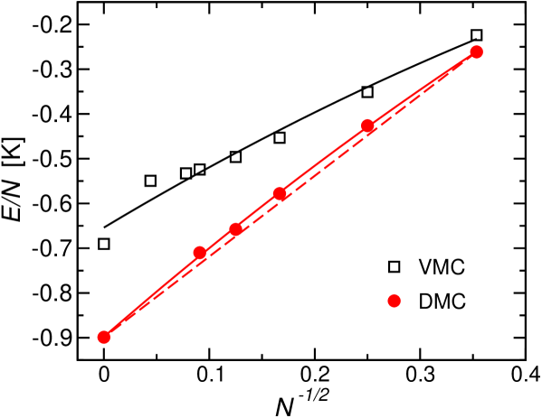
Figure 6.3: Energies per particle (in K) of $N$-atom puddles as a function of $N^{-1/2}$, obtained from our vmc (empty squares) and linear dmc (filled circles) calculations. Solid lines stand for parabolic fits to the data. The dashed line is a straight line between the $N=8$ and bulk dmc values.

We have fitted these energies to a parabolic mass formula like Eq. (6.19). The coefficients of the fit are given in Table 6.3, together with the deduced line tension.

Table 6.3: Coefficients (in K) of a parabolic fit of the mass formula, as given in Eq. (6.19). The last column displays the deduced line tension (in K Å^-1).

Method	$\varepsilon_{b}$	$\varepsilon_{l}$	$\varepsilon_{c}$	$\lambda$
vmc	$-0.654(1)$	$1.41(1)$	$-0.62(2)$	$0.083(1)$
dmc	$-0.898(2)$	$2.05(2)$	$-0.71(3)$	$0.121(1)$

Notice that the coefficient $\varepsilon_{b}$ of the dmc calculation is identical, within statistical uncertainties, to the bulk energy per particle of Table 6.2; on the contrary, the same does not happen for the vmc values. This gives us confidence on Eq. (6.19) being suitable for the fit of the dmc data. In fact, the $\chi^{2}$ of the dmc fit is very small, $\chi^{2}=5.7\times 10^{-6}$. Regarding the line tension, and despite using a different version of the Aziz potential and a different trial function, we observe that our vmc estimate is rather close to the one reported in [KC99], $\lambda_{\rm KC}=0.07$ K/Å. However, both vmc results are remarkably different from the dmc line tension that we find, namely $\lambda_{\rm DMC}=(0.121\pm 0.001)$ K/Å.

In all cases, the line energy coefficient is approximately minus twice the volume energy term, similarly to the 3D case [PPW86]. Also the curvature coefficient is not small and therefore one expects curvature effects to be important. To stress this fact, we have also plotted in the figure a straight dashed line between the $N=8$ and bulk dmc values. In fact, a linear fit of the dmc energies gives coefficients $\varepsilon_{b}=-0.885$ K and $\varepsilon_{l}=1.80$ K, which are appreciably different from the previous ones. The bulk energy extrapolated from this linear fit differs from the directly calculated value, and the corresponding line energy is closer to the variational one.

We note that in both vmc and dmc cases the extracted $\varepsilon_{c}$ is negative, i. e. the binding energy is a convex function of $z$ as it also happens for the 3D clusters [PPW86]. This is in contrast with the value of $\varepsilon_{c}$ reported in Ref. [KC99] which was positive but rather smaller in absolute value and with larger error bars. Actually, as argued in Ref. [PPW86] for 3D clusters, one would expect the curvature correction to the energy to be positive, as it corresponds physically to a lack of binding of the surface atoms due to the curvature of the surface (see Fig. 6.4) and, so, to an increase in the total energy of the system. Therefore, one should take the extracted value for $\varepsilon_{c}$ with certain caution and not emphasize its physical significance. Most probably it is due to the small size of the clusters used to build the mass formula, which ultimately forces the $E/N$ curve to approach the abscisa axis. In fact, we will see in Chapter 7 that $\varepsilon_{c}$ turns out to be positive when the smaller droplets are discarded and much larger ones are taken into account.

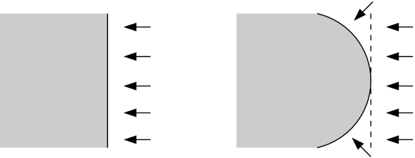
Figure 6.4: Why do we loose binding energy in a finite system? On the left side we see a semiinfinite medium (shaded region) in contact with a vacuum (white): the lack of particles on the right-hand-side (indicated by the arrows) of the interface (solid line) gives rise to a reduction of their binding energy and, therefore, also of the total binding energy of the system. On the right graph we see what happens when the interface is curved (from the dashed line to the solid one): even more binding is lost due to the further decrease in the number of neighbors for the atoms close to the frontier.

In any case, we have checked that, with the present dmc data, the value and sign of $\varepsilon_{c}$ are stable against different possible fits, e. g., changing the number of data points used to build the fit, or using a cubic mass formula. Also, the values of the two first coefficients $\varepsilon_{b},\varepsilon_{l}$ are quite robust against all performed fits. As an illustration, if one takes out the bulk point, the predicted bulk energy per particle and line tension are equal to the reported ones within 1% and 5% respectively. Therefore, we believe that the extracted line tension should be reliable, as it also happens for vmc calculations of three-dimensional clusters [PPW86], where the extracted surface tension is in agreement with the experimental one even if $\varepsilon_{c}<0$ in the fit.

6.5 vmc and dmc density profiles

6.5.1 Calculating pure estimators

The calculation of observables given by operators that do not commute with the Hamiltonian poses a new problem to the dmc method. After convergence, the walkers are distributed according to the so-called mixed probability distribution given by the product of the exact and the trial wave functions, $f(\bm{R},\tau\rightarrow\infty)=\Psi(\bm{R})\Phi_{T}(\bm{R})$. Therefore averaging the local values of the operator does not give the exact expectation value unless the operator commutes with the Hamiltonian. The result obtained by straightforward averaging is the so-called mixed estimator,

$$\langle A(\bm{R})\rangle_{\rm mixed}=\frac{\langle\Psi|A|\Phi_{T}\rangle}{\langle\Psi|\Phi_{T}\rangle}\>,$$

which is of first order error in the trial wave function. A first option devised to overcome this problem is the use of extrapolated estimators [HLR94],

$$\langle A(\bm{R})\rangle_{\rm extrapolated}=2\langle A(\bm{R})\rangle_{\rm mixed}-\langle A(\bm{R})\rangle_{\rm variational}\>,$$

where the variational estimate is calculated with $\Phi_{T}$ alone. However, also extrapolated estimates are trial-function dependent and biased [HLR94, CB95].

Several alternatives have been presented in the literature in order to obtain ‘unbiased’ or ‘pure’ (i. e., trial-function-independent and statistically exact) values. We have used the forward or future walking technique [HLR94] to calculate unbiased density profiles. The key ingredient to correct the mixed estimator is to include as a weight in the sampling the quotient $\Psi({\bf R})/\Phi_{T}({\bf R})$ for each walker,

$$\frac{\langle\Psi|A|\Psi\rangle}{\langle\Psi|\Psi\rangle}\equiv\frac{\langle\Psi|A\frac{\Psi}{\Phi_{T}}|\Phi_{T}\rangle}{\langle\Psi|\frac{\Psi}{\Phi_{T}}|\Phi_{T}\rangle}=:\langle A\rangle_{\rm pure}\>.$$

The value of this weight for each walker is given by its asymptotic number of descendants [LKC74]:

$$\frac{\Psi(\bm{R})}{\Phi_{T}(\bm{R})}=n_{\rm sons}(\bm{R};\tau\rightarrow\infty)\>.$$ (6.20)

Various algorithms have been proposed in order to compute this quantity. In this work we use an algorithm by Casulleras and Boronat [CB95] that constitutes a simple and efficient implementation of the future walking method.

Let us assume that we are already in the asymptotic regime where the usual Monte Carlo procedure would start to accumulate data to compute (mixed) averages. We define a new variable $P$ that accumulates the value of the quantity of interest, $A(\bm{R})$, for some Monte Carlo steps (labeled here by $\nu=1,\cdots,M$) within this asymptotic regime

$$P_{i}=\sum_{\nu=1}^{M}A(\bm{R}_{i}^{\nu})\>.$$

Here the same value $A(\bm{R}_{i})$ is transmitted to all descendants of walker $\bm{R}_{i}$, while the death of a walker $\bm{R}_{j}$ at any time implies that no more values will be added to the corresponding $P_{j}$ at later times. Thus, each value $A(\bm{R}_{i})$ will appear in the set of $\{P_{i}\}\leavevmode\nobreak\ (i=1,\cdots,N_{f})$ at the end of the interval as many times as descendants of the walker $\bm{R}_{i}$ have appeared, i. e., with a weight $\propto n_{\rm sons}(\bm{R}_{i})$, which is the desired one [cf. Eq. (6.20)]. Therefore, averaging $P_{i}$ at the end of this interval we have

$$\overline{P}:=\frac{1}{M\times N_{f}}\sum_{i=1}^{N_{f}}P_{i}\equiv\langle A\rangle_{\rm pure}\>.$$ (6.21)

This scheme is easily implemented in a usual dmc calculation, as one can determine a value for $\overline{P}$ at the end of each averaging block setting $M=$ number of steps in a block. At the end of the simulation, from the set of $\overline{P}$ over the different blocks we can get an estimate for $\langle A\rangle_{\rm pure}$ and its statistical uncertainty. A study of the dependence of $\overline{P}$ on $M$, typically shows an initial transient period during which the estimator ‘gets rid’ of the properties coming from the guiding function. After this period, and for a wide range of block lengths $M$, the computed average gives an unbiased estimate of the expectation value of the operator [CB95]. Therefore, studying this dependence, one can adjust $M$ so as to obtain a pure estimate with a small statistical uncertainty.

6.5.2 Numerical results

To obtain pure dmc estimates for the density profiles of ⁴He puddles, we have performed a careful analysis of the behavior of the profiles with varying block lenghts $M$ over which they were calculated. Typically, a range $M=100-1000$ has been explored, showing that for $M=500$ the computed quantity had already converged. For example, we show in Fig. 6.5 the estimated density profiles for block lengths $M=100$ (grey line) and $M=1000$ (black line). The improvement from one to the other is noticeable: the estimation obtained with a larger block length has a steeper surface, which indicates a larger line tension.

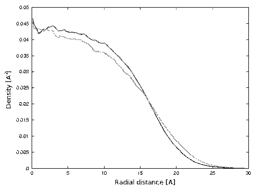
Figure 6.5: Convergence of the future walking method: density profiles for a puddle containing $N=36$ atoms as obtained by the future walking method with block lenghts $M=100$ (grey line) and $M=1000$ (black line).

The converged pure dmc estimates that we obtain in this way (with a larger number of blocks, to reduce the statistical uncertainties that show up as oscillations in the profiles in Fig. 6.5) for the density profiles of several puddles are plotted with symbols in Fig. 6.6. This figure also contains an horizontal line which indicates the saturation density of the homogeneous system, $\rho_{0}^{\textsc{dmc}}=0.04344$ Å^-2. For the puddle containing 36 atoms, the vmc profile obtained from a Gaussian Ansatz [Eq. (6.17)] is also shown as a dashed line for comparison. As one can appreciate in the figure, the process of optimization implied by the dmc method changes the profile reducing its thickness, i. e., producing a sharper surface. Indeed, by comparing this figure with Fig. 6.5 one can see how the pure estimator for $M=100$ is still influenced by the guiding function, which yields a softer boundary. This residual influence of $\Phi_{T}$ vanishes completely for $M\geq 500$ for all puddles.

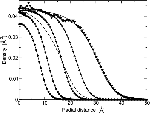
Figure 6.6: Density profiles of ⁴He puddles with various number of atoms, $N=8$ (circles), 16 (squares), 36 (diamonds), 64 (triangles up) and 121 (triangles down), obtained from our pure estimators for the linear dmc calculations. The solid horizontal line indicates the saturation density of the homogeneous system. The dashed line is the vmc profile for $N=36$ with a Gaussian trial function. The figure also contains the fits to the data provided by a generalized Fermi function, as explained in the text.

A first observation on the dmc profiles is that for the smaller clusters the central density is below $\rho_{0}$, while for the larger values of $N$ shown in the figure the central density appears to be above $\rho_{0}$, indicating a so-called leptodermous behavior [ST87b]. One expects that, increasing even more the number of particles, the central density will approach $\rho_{0}$ from above, as in the 3D case [ST87b, CK92]. It is worth noticing the oscillating behavior in the interior part of the density profile for $N=121$. It is difficult however to decide whether these oscillations are genuine or are simply due to a poor statistics in evaluating the pure estimator at short central densities. Unfortunately, to discard this last option would require an exceedingly long computing time, within the scheme of this work.

The solid lines plotted in Fig. 6.6 are fits to our dmc profiles provided by a generalized Fermi function of the form:

$$\rho(r)=\frac{\rho_{F}}{\left[1+\exp{\left(\frac{r-R}{c}\right)}\right]^{\nu}}\>.$$ (6.22)

The overall agreement with the numerical data is very good, and better than for a usual Fermi function (i. e., fixing $\nu=1$). An exception is the droplet with 121 atoms, where the oscillating behavior of the data cannot be reproduced by the fitting function. However, we have already pointed out that the physical significance of these oscillations is not clear.

The values of the parameters that best fit our data are given in Table 6.4 together with the thickness $t$ and the root mean square (rms) radius calculated with them. As usual, $t$ is defined as the distance over which the density falls from 90% to 10% of its central value; for a profile of the form of Eq. (6.22) this can be found analytically, and it turns out to depend only on $c$ and $\nu$:

$$t=c\>\ln\frac{0.1^{-1/\nu}-1}{0.9^{-1/\nu}-1}\>.$$ (6.23)

Regarding the rms radius, defined through

$$\langle r^{2}\rangle:=\frac{\int_{0}^{\infty}\mathrm{d}r\,r^{3}\rho(r)}{\int_{0}^{\infty}\mathrm{d}r\,r\rho(r)}\>,$$

we have checked that the value calculated within the dmc code and the one derived from the fit agree to better than 0.5%, except for the $N=121$ case, where the difference is 1% (most probably due to the oscillating behavior of the dmc profile).

Table 6.4: Parameters of a Fermi-profile fit to the density profiles. All lengths are in Å and $\rho_{F}$ is in Å^-2. The parameter $\nu$ is adimensional.

$N$	$\rho_{F}$	$R$	$c$	$\nu$	$t$	$\langle r^{2}\rangle^{1/2}$
$8$	$0.03740$	$9.308$	$2.156$	$1.739$	$8.166$	$7.20$
$16$	$0.04204$	$13.38$	$2.656$	$2.284$	$9.580$	$9.18$
$36$	$0.04305$	$19.47$	$3.104$	$2.400$	$11.11$	$12.91$
$64$	$0.04386$	$26.68$	$3.783$	$3.111$	$13.09$	$16.68$
$121$	$0.04304$	$40.09$	$5.566$	$4.714$	$18.52$	$23.15$

For a sharp surface ($t\ll{\langle r^{2}\rangle}^{1/2}$), one could approximate the density profile by a step function $\rho(r)=\rho_{\rm step}\Theta(r_{\rm step}-r)$. The rms radius corresponding to this profile is given by $\langle r^{2}\rangle^{1/2}=r_{\rm step}/\sqrt{2}$, so that it grows with the number of particles as $N^{1/2}$. More precisely,

$$\langle r^{2}\rangle^{1/2}=\sqrt{\frac{N}{2\pi\rho_{\rm step}}}\>.$$ (6.24)

That is, faster than in 3D, in which case grows as $N^{1/3}$. This behavior allows for an alternative determination of the saturation density by performing a fit of the calculated rms radii to the above relation. The value of $\rho_{0}$ extracted from the slope of a linear fit to the mean square radii reported in Table 6.4 is 0.042 Å^-2, in reasonable agreement (taking into account that for these droplets $t$ is not much smaller than $\langle r^{2}\rangle^{1/2}$) with the determination from the calculation for the homogeneous system. It is interesting to note that a similar treatment with the fitted values for the parameter $R$, which intuitively gives the ‘central’ point of the surface, does not give a good estimate for $\rho_{0}$ (0.012 Å^-2). In fact, $R$ seems to grow faster than $N^{1/2}$.

For these droplets, the thickness is continuously increasing with $N$. As the finite value of the thickness for the semiinfinite system should define an asymptotic value for $t$, we expect that for larger puddles the thickness will present a maximum and smoothly approach this asymptotic value from above, as happens in the 3D case [ST87b]. To check this numerically, one needs the profiles of much larger puddles, which are unaffordable in a dmc calculation. However, it is possible to find them using a Density Functional, as we will show in Chapter 7.

Finally, we also remark the asymmetric character of the density profiles with respect to the point at which the density falls at half its value at the center of the droplet. Numerically, this behavior is reflected in the value of $\nu$, which grows with $N$, and also in the increasing difference between the quantities $R$ and $\langle r^{2}\rangle^{1/2}$.

6.6 Summary and conclusions

In this chapter we have considered strictly two-dimensional systems of liquid ⁴He, which are of course an idealization of a real quantum film. They are nevertheless interesting because their study can enlighten the underlying structure of real quasi-2D systems. Of course, in the latter case, one has to take also into account the interaction with the substrate, which basically provides a global attractive potential. In the ideal 2D case, the suppression of the wave function component in the third dimension, produces an increment of the global repulsion between atoms, resulting in a smaller binding energy per particle, and a decrease of the equilibrium density [AK02].

We have calculated the binding energies of two-dimensional ⁴He clusters by means of a diffusion Monte Carlo method, and we have seen that they can be well fitted by a mass formula in powers of $z=N^{-1/2}$. The analysis of the mass formula provides the value $\lambda=0.121$ K/Å for the line tension, which significantly differs from the one obtained from a similar analysis of vmc data and the one previously reported in the literature [KC99]. The quadratic term of the mass formula cannot be neglected and results in a negative value of the curvature energy, similarly to what happens in the 3D case [PPW86, CK92]. However, the studied clusters may be too small to give physical significance to this result.

The density profiles obtained with the pure estimator have been fitted to a generalized Fermi function, and the behavior of the rms radius and the thickness, as well as the asymmetric character of the profile as a function of $N$ have been discussed.

Due to computing limitations on dmc calculations, we have restricted our study to relatively small clusters with $N\leq 121$ atoms. However, to fully understand the transition from finite clusters to the bulk medium, both for the energetics and the structure of the profiles, it seems interesting to have results for much larger $N$. We will explore these cases in the next chapter by means of a density functional theory.

Chapter 7 Density Functional study of two-dimensional ⁴He non-homogeneous systems

Per jo, que sabia el cant secret de l’aigua,
les lloances del foc, de la gleva i del vent,
s c endinsat en obscura pres ,
vaig devallar per esglaons de pedra
al clos recinte de llises parets
i avan o sol a l’esglai del llarg crit
que deia per les voltes el meu nom.

Salvador Espriu, dins Final del laberint

7.1 Introduction to Density Functional theory

In this chapter we continue the study of two-dimensional ⁴He systems initiated in Chapter 6 by analyzing the energetics and structure of the semi-infinite medium and slabs. Also, we will take a look at clusters larger than those studied by means of the dmc technique in order to clarify some of the points that have not been fully understood previously, e. g., the sign and value of the curvature energy $\varepsilon_{c}$ in the mass formula, or the behavior of the surface thickness when approaching the bulk medium.

As it is well know, large systems are difficult to tackle with Monte Carlo methods as these deal with all $d\times N$ coordinates of the system components ($d=$ dimensionality of the system, $N=$ number of constituents of the system). There are several alternative approximate methods, from mean-field calculations, where the many-body wave function is written as a direct product of single-particle wave functions, with the appropriate symmetry properties related to the quantum-statistical character of the particles, to more involved techniques such as correlated basis functions (cbf) or the coupled-cluster method (ccm). A very good reference to have an overview of the power and flaws of all these techniques can be found in Ref. [FFK02]. Here we will make use of the Density Functional (df) theory, which unites the power of computationally simple calculations with an insight to the physics of the problem.

7.1.1 The Hohenberg-Kohn theorem

The basis of the Density Functional theory relies on the famous Hohenberg-Kohn theorem which states that the ground state energy of a many-body system is determined solely by its one-body density $\rho(\bm{r})$ [HK64, FNM03]. In other words, the ground-state energy can be written as a functional of the density, $E=E[\rho]$.

Unfortunately, the Hohenberg-Kohn theorem does not tell how to build this functional; it is just an existence theorem. We need to resort to our understanding of the problem to build it, which can be done in different ways. In the context of quantum liquids, one usually follows a ‘phenomenological’ approach: based on the available physical information on the problem, one defines a density functional

$$E[\rho]=\int\mathrm{d}^{3}r\,\varepsilon[\rho(\bm{r})]\>,$$ (7.1)

through an energy density $\varepsilon[\rho]$. The corresponding ground state is then found by functional minimization, usually restricted by the normalization of the density. This condition introduces the chemical potential into the problem as a Lagrange multiplier, namely

$$\frac{\delta E}{\delta\rho}=\mu\>.$$ (7.2)

Several functionals have been proposed to study helium systems, either pure ⁴He or ³He or mixtures thereof, see e. g. [Str85, ST87a, BJH⁺93, DLP⁺95, Szy00]. The density functional we shall use is the simplest version of the zero-range functional intensively used in 3D calculations [Str85]. We have adjusted its parameters so as to reproduce some properties of the ground state of the homogeneous two-dimensional system as obtained in dmc calculations [GBC96a], as well as the line tension extracted from the mass formula in the previous chapter. This procedure is discussed in Section 7.2, together with the results for the slabs. Section 7.3 is devoted to the study of finite droplets, with special emphasis for those with a large number of atoms. In Section 7.4 a short discussion on hydrodynamic equilibrium in a droplet is presented, followed in Section 7.5 by a comparison of the obtained results with those of other qmc and df calculations in 3D and 2D. Finally, in Section 7.6 the main conclusions are summarized.

7.2 Semi-infinite system and slabs

Density functionals to investigate surface properties of superfluid ⁴He were developed during the 1970’s [ES75]. At zero temperature and in the absence of currents, the order parameter of a bosonic system can be identified simply as the square root of the one-body density $\rho(\bm{r})$, so it is natural to think of the energy of the system as a functional of the helium density. In analogy with the formalism of zero-range Skyrme interactions in nuclear physics [VB72], Stringari proposed a zero-range density functional for non-homogeneous three-dimensional ³He systems [Str85]. A similar form,

$$E[\rho]=\int\,\mathrm{d}^{2}r\left\{\frac{\hbar^{2}}{2m}\frac{|\nabla\rho|^{2}}{4\rho}+b\rho^{2}+c\rho^{2+\gamma}+d|\nabla\rho|^{2}\right\},$$ (7.3)

was soon used to study ⁴He surface properties [ST87a] and clusters [ST87b].

For the two-dimensional systems of our interest, we will use the same functional form. However, the parameters $\{b,c,\gamma\}$ characterizing the functional for homogeneous systems have to be recalculated by requiring that the functional reproduces some known properties of the two-dimensional ⁴He system, such as the ground-state energy per particle ($e_{0}=-0.89706$ K), and the saturation density ($\rho_{0}=0.04344$ Å^-2), which have been determined in the framework of the Diffusion Monte Carlo method [GBC96a, SMPN03] (see also Chapter 6). For the homogeneous system, the gradient terms in (7.3) vanish in the ground state, and one gets

$$e_{0} =b\rho_{0}+c\rho_{0}^{1+\gamma}$$

$$0 =b+(1+\gamma)c\rho_{0}^{\gamma}\>.$$

The third equation used to fix the parameters $\{b,c,\gamma\}$ is obtained by imposing the known value of the speed of sound at saturation, $s=92.8$ m/s [GBC96a]. This is related to the compressibility $\kappa$ of the system, and one can write it as

$$ms^{2}=\frac{1}{\kappa\rho_{0}}=\left.\frac{\partial}{\partial\rho}\left(\rho^{2}\frac{\partial e}{\partial\rho}\right)\right|_{\rho_{0}}=2b\rho_{0}+(1+\gamma)(2+\gamma)c\rho_{0}^{1+\gamma}\>.$$

Finally, the parameter $d$ is fixed by demanding that the line tension of the semi-infinite system equals that obtained from dmc calculations for 2D clusters, $\lambda_{\rm DMC}=0.121$ K/Å (see Ch. 6 of this thesis). The behavior of the energy per particle as a function of density for the homogeneous system provided by this functional reproduces very well the equation of state obtained from dmc calculations in a wide range of densities [GBC96a, NMPS03]. As a first step in understanding non-homogeneous systems, we will consider the semi-infinite system.

In order to determine the density profile $\rho(\bm{r})$, in principle one should solve the Euler-Lagrange equation (7.2) that results from minimizing the energy functional (7.3). One should also introduce the Lagrange multiplier $\mu$, which ensures the normalization of the density to the desired number of particles, and that is to be identified with the chemical potential of the system,

$$\frac{\hbar^{2}}{8m}\left[-\frac{2\nabla^{2}\rho}{\rho}+\frac{|\nabla\rho|^{2}}{\rho^{2}}\right]+2b\rho+(2+\gamma)c\rho^{1+\gamma}-2d\nabla^{2}\rho=\mu\;.$$ (7.4)

One should also impose the boundary conditions $\rho(x\rightarrow-\infty)=\rho_{0}$ and $\rho^{\prime}(x\rightarrow-\infty)=0$, where the prime denotes derivative with respect to $x$, the coordinate perpendicular to the surface of the system (cf. Fig. 7.1).

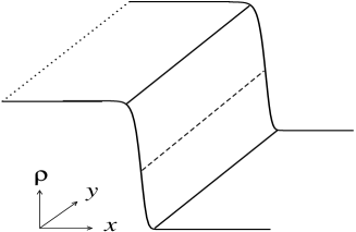
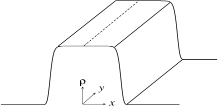
Figure 7.1: Sketches of the semi-infinite medium and a slab: the $x$ axis is perpendicular to the surfaces, the $y$ axis the symmetry axis. The dashed line indicates the projection of the $y$ axis on the density profile: at $\rho_{0}/2$ for the semi-infinite medium and at $\rho_{c}$ for the slab.

For the particular case of a zero-range functional (7.3), the line tension can be evaluated in a closed form, i. e., without solving for the density profile:

$$\lambda(d)=2\int_{0}^{\rho_{0}}\;\mathrm{d}\rho\left[\left(\frac{\hbar^{2}}{8m}+\rho d\right)\left(b\rho+c\rho^{1+\gamma}-\mu\right)\right]^{1/2}\;.$$ (7.5)

Then, imposing $\lambda(d)=\lambda_{\rm DMC}$, one gets an implicit equation for $d$ which can be solved numerically, thus yielding the last parameter of the functional. The parameters for the two-dimensional zero-range functional fixed in this way are listed in Table 7.1.

Table 7.1: Parameters of the two-dimensional zero-range functional (7.3).

$b=-26.35$ KÅ2	$\gamma=3.62$
$c=4.88\times 10^{5}$ KÅ2(1+γ)	$d=359$ KÅ4

Once the functional is defined, one can study any two-dimensional ⁴He system. The first systems we have considered are two-dimensional slabs with varying central density $\rho_{c}=\rho(x=0)$ (see Fig. 7.1). For later reference, we note that a systematic study of three-dimensional ⁴He slabs with different density functionals has been presented in Ref. [Szy00]. The Euler equation for the slabs is the same as for the semi-infinite system [Eq. (7.4)]. The changes in the solution of the equation originate from the different geometry and boundary conditions which define the slab; in particular, the slab has two surfaces, while the semi-infinite medium only has one (located around $x=0$). Translational symmetry implies that the density depends only on the coordinate perpendicular to the slab surface, which we call $x$ again. Then, $\nabla\rho=\rho^{\prime}(x)$ and $\nabla^{2}\rho=\rho^{\prime\prime}(x)$. In this way, the Euler equation (7.4) can be expressed in a more convenient form, in which now $\rho$ depends only on $x$,

$$\frac{\hbar^{2}}{8m}\left(-\frac{2\rho^{\prime\prime}}{\rho}+\frac{(\rho^{\prime})^{2}}{\rho^{2}}\right)+2b\rho+(2+\gamma)c\rho^{1+\gamma}-2d\rho^{\prime\prime}=\mu$$ (7.6)

The expression in parenthesis can be rewritten as a total derivative multiplying it by $\rho^{\prime}$,

$$\left(\frac{2\rho^{\prime\prime}}{\rho}-\frac{(\rho^{\prime})^{2}}{\rho^{2}}\right)\rho^{\prime}=\left(\frac{2\rho^{\prime}\rho^{\prime\prime}}{\rho}-\frac{(\rho^{\prime})^{3}}{\rho^{2}}\right)=\frac{d}{dx}\left(\frac{(\rho^{\prime})^{2}}{\rho}\right)\>.$$

Thus, one can eliminate the second derivative of Eq. (7.6) by multiplying both sides of the equation by $\rho^{\prime}$ and integrating with respect to $x$, from the origin to a given value of $x$,

$$\left[-\frac{\hbar^{2}}{8m}\frac{(\rho^{\prime})^{2}}{\rho}+b\rho^{2}+c\rho^{\gamma+2}-d(\rho^{\prime})^{2}\right]_{0}^{x}=\mu\left[\rho(x)-\rho(0)\right]\>.$$ (7.7)

Imposing the boundary conditions $\rho(\infty)=\rho^{\prime}(\infty)=0$, and considering that the slab is symmetric under inversion of the $x$-axis, and therefore $\rho^{\prime}(0)=0$, one finds that the chemical potential as a function of the central density of the slab reads

$$\mu=b\rho_{c}+c\rho_{c}^{\gamma+1}.$$ (7.8)

It is worth to remind that this chemical potential is constant along the profile.

Going back to Eq. (7.7), and using again the fact that $\rho^{\prime}(0)=0$, one obtains

$$|\rho^{\prime}|=\sqrt{\frac{\rho^{2}(b\rho+c\rho^{\gamma+1}-\mu)}{\frac{\hbar^{2}}{8m}+d\rho}}.$$ (7.9)

This expression for $\rho^{\prime}$ is then used to calculate the number of atoms per unit length along the $y$ axis (that is, the coverage) in a closed expression in terms of the density

$$\frac{N}{L}=2\int_{0}^{\infty}\rho(x)\mathrm{d}x=2\int_{0}^{\rho(0)}\rho\frac{\mathrm{d}\rho}{|\rho^{\prime}|}=2\int_{0}^{\rho(0)}\mathrm{d}\rho\sqrt{\frac{\frac{\hbar^{2}}{8m}+d\rho}{b\rho+c\rho^{1+\gamma}-\mu}}\>,$$

where the factor 2 takes into account the symmetry of the slab under the transformation $x\rightarrow-x$. This integral has a singularity when $\rho\rightarrow\rho_{c}$ that can be avoided integrating by parts. The final expression, free of numerical problems, reads

$$\frac{N}{L}=-\frac{4}{b}\sqrt{-\frac{\hbar^{2}}{8m}\mu}\\ -4\int_{0}^{\rho_{c}}\!\!\mathrm{d}\rho\frac{\sqrt{b\rho+c\rho^{1+\gamma}-\mu}\left\{\frac{d}{2}[b+c(1+\gamma)\rho^{\gamma}]-(\frac{\hbar^{2}}{8m}+d\rho)c\gamma(1+\gamma)\rho^{\gamma-1}\right\}}{[b+c(1+\gamma)\rho^{\gamma}]^{2}\leavevmode\nobreak\ (\frac{\hbar^{2}}{8m}+d\rho)^{1/2}}.$$

Also useful is the energy per unit length,

$$\frac{E}{L}=2\int_{0}^{\infty}\mathrm{d}x\left[\frac{\hbar^{2}}{8m}\frac{(\rho^{\prime})^{2}}{\rho}+b\rho^{2}+c\rho^{2+\gamma}+d(\rho^{\prime})^{2}\right].$$

Using Eq. (7.9) and the previous definition of the coverage, one can finally express the energy per particle $e=E/N$ in terms of the inverse of the coverage, $\widetilde{x}:=L/N$,

$$e(\widetilde{x})=\mu(\widetilde{x})+4\widetilde{x}\int_{0}^{\rho(0)}\mathrm{d}\rho\sqrt{\left(\frac{\hbar^{2}}{8m}+d\rho\right)[b\rho+c\rho^{1+\gamma}-\mu(\widetilde{x})]}$$ (7.10)

Therefore, given a central density $\rho_{c}\in[0,\rho_{0}]$, one can calculate the chemical potential, the coverage and the energy per particle of the corresponding slab.

The energy per particle and the chemical potential for ⁴He slabs are reported in Fig. 7.2 as a function of the inverse of the coverage $\widetilde{x}$.

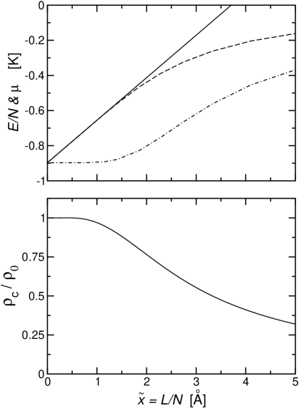
Figure 7.2: (Top) Energy per particle (dashed line) and chemical potential (dot-dashed line) in kelvin for ⁴He slabs as a function of the inverse of the coverage $\widetilde{x}$ (in Å). The slope of the solid line is twice the line tension of the semi-infinite medium, which corresponds to the asymptotic $\widetilde{x}\rightarrow 0$ behavior of the energy per particle [see Eq. (7.11)]. (Bottom) Ratio between the central density $\rho_{c}$ and the bulk equilibrium density for ⁴He slabs as a function of the inverse of the coverage.

In the limit $\widetilde{x}\rightarrow 0$ one recovers the binding energy of the uniform system at $\rho_{0}$, which in turn coincides with the chemical potential. The energy per particle has a very clean linear behavior at the origin as illustrated by the solid straight line which provides a very good description of the energy per particle up to $\widetilde{x}\sim 1.5$ Å. The slope of this line can be analytically derived and turns out to be twice the line tension, which acts to reduce the binding energy per particle of the slab when increasing the inverse of the coverage. The derivation of this limiting behavior of the energy per particle can be easily obtained starting from Eq. (7.10), which defines the energy per particle as a function of $\widetilde{x}$, by performing an expansion around $\widetilde{x}=0$. The leading terms result in

$$e(\widetilde{x})=\mu_{\infty}+2\lambda\widetilde{x}+\cdots$$ (7.11)

For values $\widetilde{x}\gtrsim 1.5$ Å the energy per particle starts to bend horizontally and becomes a convex function, approaching zero very slowly.

In contrast, the chemical potential is very flat at the origin, being determined by the central density of the slab [cf. Eq. (7.8)], which varies only slightly for small $\widetilde{x}$. This can be seen in the lower panel of Fig. 7.2, which displays the ratio of the central density of the slabs to the equilibrium density as a function of the inverse of the coverage. In agreement with the chemical potential, the central density is very flat at small values of $\widetilde{x}$. The flatness of the central density and the chemical potential for small values of $\widetilde{x}$, indicates that the slab approaches very slowly the limit of the infinite system.

Note that the central density of a slab can never go above the equilibrium density and is always a decreasing function of $\widetilde{x}$. More generally, the density profiles of the slabs can be obtained from Eq. (7.9), which we now rewrite as

$$x=\int_{\rho_{c}}^{\rho(x)}\mathrm{d}\rho\left(\frac{d\rho}{dx}\right)^{-1}=\int_{\rho(x)}^{\rho_{c}}\mathrm{d}\rho\left[\frac{\frac{\hbar^{2}}{8m}\frac{1}{\rho}+d}{b\rho^{2}+c\rho^{2+\gamma}-\mu\rho}\right]^{1/2}\;,$$ (7.12)

valid for $x\geq 0$. The profile for $x<0$ is found by symmetry. Notice the presence again of a divergence when $\rho\rightarrow\rho_{c}$ which can also be avoided integrating by parts. The profiles calculated for various central densities are plotted in Fig. 7.3.

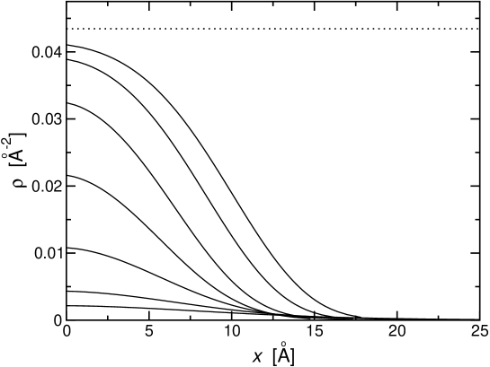
Figure 7.3: Density profiles for ⁴He slabs with central densities $\rho_{c}/\rho_{0}$=0.05, 0.1, 0.25, 0.5, 0.75, 0.9, 0.95, where $\rho_{0}$ is the equilibrium density of the bulk, indicated by the horizontal dotted line.

The size of the slab increases with the central density. A measure of this size is given by the radius $R_{1/2}$, defined as the distance from the origin to the point where the density has decreased to half its central value. This quantity is shown on the left panel of Fig. 7.4 as a function of $\widetilde{x}$.

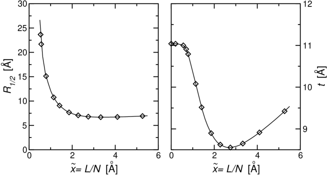
Figure 7.4: Radius (left panel) and thickness (right panel) of ⁴He slabs as a function of $\widetilde{x}$. The symbols are the calculated data while the lines are cubic splines to guide the eye.

As expected, it diverges in the limit $\rho_{c}\rightarrow\rho_{0}$ and is mainly a decreasing function of $\widetilde{x}$. However, it also presents a very shallow minimum around $\widetilde{x}\sim 3.3$ Å, after which it grows slightly. Physically, one can understand this last feature from the fact that for $\widetilde{x}>3$ Å the density of the system is everywhere small (cf. Figs. 7.2–7.3): each particle will have very few others to attach to, and the slab will become more extended.

The profiles are also characterized by the thickness $t$, defined as the distance between the points where the density has decreased from $90\%$ to $10\%$ of its central value. The dependence of the thickness on $\widetilde{x}$ is shown on the right part of Fig. 7.4. Up to $\widetilde{x}\sim 1$, the thickness is a pretty flat function, indicating that the surface of the slab is very much the same, and is actually the radius of the slab that grows very fast and diverges when $\widetilde{x}\rightarrow 0$. The thickness is large for the slabs with larger $\widetilde{x}$ again due to the low density of these systems. When the central density is increased ($\widetilde{x}$ decreases), the thickness decreases until it has a minimum at $\widetilde{x}\approx 2.75$ Å, with $t\approx 8.6$ Å. Then, it increases again approaching a finite value at the origin, corresponding to the semi-infinite medium, $t\approx 11.03$ Å. It is interesting to note the plateau that appears for $\widetilde{x}<1$, which may be related to the analogous behavior for the central density (cf. Fig. 7.2): the slabs are in many aspects similar to the semi-infinite system already for $\widetilde{x}\approx 1$. However, other properties (most importantly, the energy per particle) do need to go to the limit $\widetilde{x}\rightarrow 0$ to get rid of its finite-size dependencies. On the other hand, for $\widetilde{x}>3$ the slabs seem to change from a strongly correlated behavior over to a more ‘dilute’ one.

7.3 Drops and line tension

As a next step, we consider drops of a fixed number of atoms $N$. These where already studied by dmc techniques in Chapter 6. However, computational limitations allowed us to study only small values of $N$. Here, we will take advantage of the computational feasibility of the Density Functional calculations and will extend the analysis to much greater $N$. In this way it will be possible to study the asymptotic behavior of several quantities which characterize the drops.

Equation (7.4) for the profile can be rewriten in the form of a Schrödinger-like equation for $\rho$:

$$\widehat{\cal H}\rho\equiv-\frac{\hbar^{2}}{4m}\left[\nabla^{2}\rho-\frac{|\nabla\rho|^{2}}{2\rho}\right]+2b\rho^{2}+(2+\gamma)c\rho^{2+\gamma}-2d\rho\nabla^{2}\rho=\mu\rho$$ (7.13)

As the number of atoms in a droplet is a well defined $N$, one would need to be very careful in determining the central density $\rho(0)$ so that the chemical potential adjusted exactly to $N$. However, it turns out that this equation is more efficiently solved by means of the steepest descent method [DFKW80]. An initial trial $\rho_{\rm input}(r)$ is projected onto the mininum of the functional by propagating it in imaginary time $\tau$. In practice, one chooses a small time step $\Delta\tau$ and iterates the equation

$$\rho(r,\tau+\Delta\tau) \approx\rho(r,\tau)-\Delta\tau\,\widehat{\cal H}\rho(r,\tau)$$ (7.14)

$$\rho(r,0) \equiv\rho_{\rm input}(r)\>,$$

normalizing $\rho$ to the total number of atoms at each iteration. The time step $\Delta\tau$ that governs the rate of convergence should be taken appropriately small in such a way that Eq. (7.14) is a valid approximation. Convergence is reached when the local chemical potential —defined as the value of $[\widehat{\cal H}\rho]/\rho$— has a constant value independent of position. In our calculations, typical values have been $\Delta\tau\sim 10^{-5}$, and some 10⁶ iterations have been necessary to reach convergence. This large number of iterations does not translate into long runs, as the local nature of the functional allows for fast calculations. Nevertheless, it is also possible that including in Eq. (7.14) second or higher orders in $\Delta\tau$, the computation might speed up, which we have not attempted.

The energy per particle (empty circles) and the chemical potential (full circles) calculated for drops with $N=16$, 36, 64, 121, 512, $1\,024$, $2\,500$ and $10\,000$ atoms are reported in Fig. 7.5 as a function of $N^{-1/2}$. Also shown for comparison are the dmc energies (empty squares) and their quadratic fit to a mass formula calculated in Chapter 6.

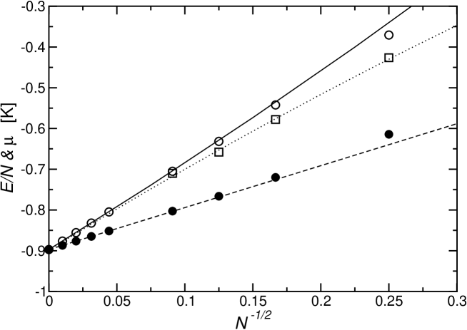
Figure 7.5: Energy per particle (empty circles) and chemical potential (full circles) of ⁴He droplets as a function of $z=N^{-1/2}$. Also shown is a quadratic fit (see text) of the results with $N\geq 512$ (solid line). The straight short-dashed line is obtained when the mass formula (with terms up to $z^{2}$) is used to calculate the chemical potential. The empty squares are the dmc energies from Chapter 6, and the dotted line corresponds to the quadratic fit to these results reported there.

The calculated energies of the droplets can again be represented very accurately with a mass formula of the type [cf. Eq. (6.19)]

$$e(N)=\varepsilon_{b}+\varepsilon_{l}z+\varepsilon_{c}z^{2}+\cdots \leavevmode\nobreak\ \leavevmode\nobreak\ \leavevmode\nobreak\ \leavevmode\nobreak\ \leavevmode\nobreak\ (z=N^{-1/2}).$$ (7.15)

Contrary to the dmc calculations, where the largest droplet that we studied had 121 atoms, here we have considered puddles with up to $10\,000$ atoms. In this way we can accurately study the behavior of the energy per particle for small values of $z$. Doing a quadratic fit to the calculated energies per particle for $N\geq 512$ and including also the bulk binding energy for $z=0$ one gets

$$y=-0.897+2.0587z+0.66466z^{2},$$ (7.16)

which is plotted by a solid line in the figure. One sees that $\varepsilon_{b}$ accurately reproduces the bulk energy per particle, which was used to fix the parameters of the functional; we note that a similar agreement was found for the dmc fit parameters (see Table 6.3). The value of $\varepsilon_{l}=2.0587$ (cf. $\epsilon_{l}=2.05$ K for the dmc fit) corresponds to a line tension $\lambda=0.121$ K/Å, which is the same as the value of the line tension of the semi-infinite system, used to build the density functional. Note, however, that the fit, even if it has been calculated with the data for $N\geq 512$, is rather accurate down to $N=36$. Obviously, one can not expect a good agreement for $N=16$, which is a system where finite-size effects are very important.

The linear behavior of the chemical potential as a function of $z$ contrasts with the plateau that was found for the slabs. This linearity is easy to understand using the mass formula (7.15) and the thermodynamic definition of the chemical potential $\mu=\partial E/\partial N$, where $E$ is the total energy of the droplet. With this prescription, the slope of the chemical potential as a function of $z$ results to be $\varepsilon_{l}/2$. This behavior is illustrated by the short-dashed line in the figure, which nicely follows the calculated data down to $N=36$. A similar analysis for the three-dimensional case, would provide a behavior of the chemical potential as a function of $z=N^{-1/3}$ dominated also by a linear component, but with a slope at the origin given by $2\varepsilon_{s}/3$, where $\varepsilon_{s}$ is the surface energy associated to three-dimensional clusters [ST87b].

It is interesting to remark that the coefficient of $z^{2}$ is positive. This sign corresponds to the expected loose of binding energy associated to the curvature of the contour of the cluster (cf. Fig. 6.4), and it is in contrast with the value of $\varepsilon_{c}$ obtained by fitting the dmc results (see Table 6.3). However, in that case the number of particles in the clusters used to build the fit was much smaller, being $N=121$ the largest number of particles and going down to N=8 for the smallest one. In the present fit we have explicitly avoided the clusters with a small number of particles which can easily distort the results and we have considered only the cases with $N\geq 512$.

Next thing to analyze are the density profiles, which we report in Fig. 7.6 for different numbers of atoms.

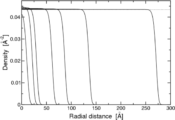
Figure 7.6: Density profiles for ⁴He droplets for $N$=16, 64, 121, 512, $1\,024$, $2\,500$ and $10\,000$ atoms as fitted to a generalized Fermi profiles [see Eq. (7.17) and Table 7.2]. The dotted horizontal line indicates the equilibrium density of the homogeneous system $\rho_{0}$.

Contrary to the slabs, the central density of the droplets can be higher than the saturation density, which is indicated in the figure by an horizontal line. The profiles are well adjusted by a generalized Fermi function,

$$\rho(r)=\frac{\rho_{F}}{\left[1+e^{\frac{r-R}{c}}\right]^{\nu}}\>,$$ (7.17)

which has an associated central density $\rho(0)=\rho_{F}/[1+e^{-R/c}]^{\nu}$. The parameters fitting the profiles for the different clusters are quoted in Table 7.2, together with the thickness and root-mean-square radius obtained thereof.

Table 7.2: Parameters of a generalized Fermi-profile fit [Eq. (7.17)] to the density profiles obtained with the zero-range density functional. All lengths are in Å and $\rho_{F}$ is in Å^-2. The parameter $\nu$ is adimensional.

$N$	$\rho_{F}$	$R$	$c$	$\nu$	$t$	$\langle r^{2}\rangle^{1/2}$
$16$	$0.04321$	$13.2718$	$3.22067$	$2.13417$	$11.746$	$9.664$
$36$	$0.04494$	$19.1852$	$3.22054$	$2.37516$	$11.548$	$12.793$
$64$	$0.04974$	$24.6826$	$3.16845$	$2.37072$	$11.364$	$16.276$
$121$	$0.04441$	$32.8314$	$3.12302$	$2.33636$	$11.226$	$21.721$
$512$	$0.04392$	$64.4245$	$3.08867$	$2.32368$	$11.112$	$43.533$
$1\,024$	$0.04378$	$89.8497$	$3.08584$	$2.32997$	$11.097$	$61.342$
$2\,500$	$0.04366$	$138.628$	$3.08552$	$2.33826$	$11.090$	$95.678$
$10\,000$	$0.04355$	$274.026$	$3.08653$	$2.34670$	$11.088$	$191.276$

The left panel of Fig. 7.7 reports the central density of the different droplets as a function of $z$. For large values of $N$, $\rho(0)$ is larger than the saturation density, i. e. the central part of the droplet is more compressed than the bulk system, which is sometimes referred to as a leptodermous behavior [ST87b]. Of course, for $N\rightarrow\infty$ the central density tends to $\rho_{0}$. First, $\rho(0)$ grows almost linearly with $z$, reaches a maximum, for $z\approx 0.13$ ($N\approx 60$), which would correspond to the most compressed droplet and, finally, for $N\leq 25$, the central region of the droplets becomes rapidly less compressed than the bulk system.

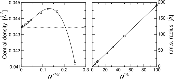
Figure 7.7: (Left) Central density of ⁴He droplets as a function of $z=N^{-1/2}$. The empty circles correspond to the results obtained with the zero-range density functional, while the line stands for a cubic spline fit to these data. The dotted horizontal line indicates the saturation density $\rho_{0}$. (Right) Root-mean-square radius of ⁴He droplets as a function of $N^{1/2}$. The solid line is a linear fit to the data without independent term. The empty circles correspond to the results of the zero-range density functional.

The root-mean-square (rms) radius corresponding to the profiles is shown in the right panel of Fig. 7.7 as a function of $N^{1/2}$. The expected linear behavior, associated to a constant average density [cf. Eq. (6.24)],

$$\langle r^{2}\rangle^{1/2}=\frac{1}{\sqrt{2\pi\overline{\rho}_{0}}}N^{1/2}\>,$$ (7.18)

is rather apparent. A linear fit to the calculated values (without independent term), from $N=16$ to $N=10\,000$, provides $\overline{\rho}_{0}=0.0434$ Å^-2, in very good agreement with the bulk equilibrium density used to fix the parameters of the density functional.

7.4 Hydrodynamic equilibrium in a droplet

We proceed now to analyze the hydrodynamic equilibrium in these helium drops. To this end, it may be interesting to analyze the pressure in one of these clusters. The study of fluid interfaces goes back to Gibbs [Gib61]. However, a clear definition of local thermodynamic variables has not yet been reached. It has been established that, across an interface, some variables (such as the chemical potential) must remain constant, while for others (such as the pressure) this is not so, and an unambiguous definition is lacking for the latter, even though there have been several attempts in recent years [TGW⁺84, Row93, Row94, LB97, MBL97, OBvM⁺99, HI02]. The usual thermodynamic expression for the pressure at zero temperature is

$$p=-\left(\frac{\partial E}{\partial V}\right)_{N}=\rho^{2}\left(\frac{\partial e}{\partial\rho}\right)_{N}=\rho(\mu-e)\>,$$

where we also used the definition of the chemical potential, $\mu=(\partial E/\partial N)_{V}$, $e$ stands for the energy per particle and $\mu$ is the chemical potential, constant throughout the system. This expression depends only on intensive variables, and is therefore appropriate to introduce the concept of local pressure in a finite system.

For our simple zero-range density functional (7.3), the energy per particle can be written as a function of the density thus

$$e(\rho)=\frac{\hbar^{2}}{8m}\frac{\left(\nabla\rho\right)^{2}}{\rho^{2}}+b\rho+c\rho^{1+\gamma}+d\frac{\left(\nabla\rho\right)^{2}}{\rho}\>,$$

which, combined with the equation above, will define a ‘pressure profile’ $p(r)$. Moreover, all the contributions to $e(\rho)$ as well as $\mu\rho$ are quantities computed during the imaginary-time evolution towards the ground state. Therefore, the evaluation of $p(r)$ does not require any further computational effort.

The calculated $p(r)$ for two sample droplets ($N=36,\leavevmode\nobreak\ 10\,000$) is shown as a function of a rescaled radial distance $r/R$ in Fig. 7.8, with $R$ the fitting parameter of Table 7.2.

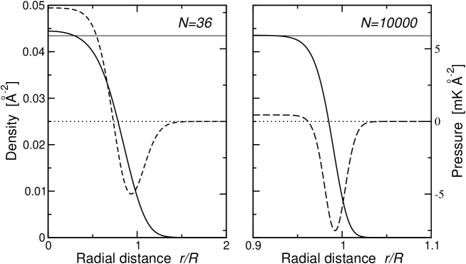
Figure 7.8: Pressure profile in the clusters with $N=36$ (left) and $N=10\,000$ (right) atoms: the solid lines are the density profiles (left ordinate axes) while the dashed lines are the calculated pressure profiles (right ordinate axis). The thin horizontal lines indicate the saturation density $\rho_{0}$ and the dotted lines mean zero pressure.

The value $p=0$ outside the drop is due to the fact that we are working in a vacuum at zero temperature, and therefore there is no vapor pressure exerted on the drop. The positive value of $p$ in the innermost region of the droplet is related to the density there being larger than the saturation density. This behavior is also expected from the Young-Laplace law for a liquid-vapor interface, that relates the pressures in the bulk of each phase with the surface tension $\lambda$ and the mean curvature radius $R_{\rm curv}$ of the interface [MBL97, Saf03]. For the case of cylindrical symmetry,

$$p_{\rm liq}=p_{\rm vap}+\frac{\lambda}{R_{\rm curv}}\>.$$ (7.19)

As mentioned above, in the zero temperature case $p_{\rm vap}=0$. The fact that the regions where $p>0$ and $\rho>\rho_{0}$ do not coincide exactly is due to the gradient terms of the Density Functional, that are not present for the homogeneous case that fixes $\rho_{0}$. Using now Eq. (7.19) with $\lambda=\lambda_{\rm DMC}$ and the calculated values $p(0)=7.82$ mK/Ų ($N=36$) and $p(0)=0.447$ mK/Ų ($N=10\,000$) as the values of the pressure in the liquid phase, we find the values for the curvature radii of the clusters with $N=36$ and $10\,000$ atoms to be $R_{\rm curv}=15.5$ Å and $R_{\rm curv}=271$ Å, which are rather close to the $R$-values from the Fermi-profile fit (see Table 7.2). This can be seen as an indication of the validity of our definition for $p(r)$, specially for large drops, where the hypothesis of a sharp interface that resides in the Young-Laplace law is better.

Close to the surface, we find a negative value for the pressure, that is, there is a tension located near the free surface of the puddle. This is especially clear for the larger drop, where the region where $p<0$ is closely restricted around the surface (note the difference in scales on the $x$-axes of both figures), while for the $N=36$ system the separation between a bulk and a surface regions is not easy to ascertain. Similar results have been found in various Molecular Dynamics calculations for liquid-vapor interfaces of different geometries (planar, cylindrical), even if using a variety of definitions for the local pressure (see, e. g., [TGW⁺84, MBL97]).

This picture of the pressure profile can be made more physically appealing by interpreting it in terms of hydrodynamic equilibrium. To this end, let us analyze the forces exerted on an area of a drop as depicted on the left panel of Fig. 7.9.

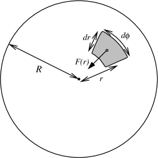
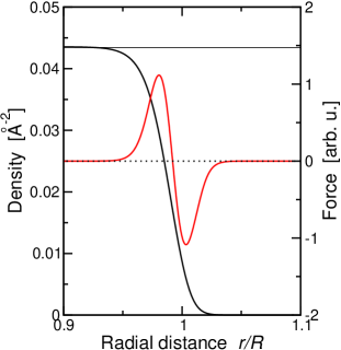
Figure 7.9: (Left) $F(r)$ stands for the effective force that keeps the drop bound. (Right) The density profile (black line) and the effective force $F(r)$ (red line) calculated to keep the drop with $N=10\,000$ atoms in equilibrium, see Eq. (7.20).

The area will be in equilibrium if there exists a force $F$ that balances the pressure difference on the two sides. This force must satisfy

$$F(r) =-r\,d\phi\,[p(r+\frac{dr}{2})-p(r-\frac{dr}{2})]=-r\,d\phi\frac{dp}{dr}\,dr=-dA\frac{dp}{dr}\>,$$ (7.20)

where $dA$ is the surface of the shaded area, and the sign convention is such that $F>0$ pulls atoms to the center of the puddle. This force is ultimately determined by the He-He interaction.

Thus, the pressure profile can be mapped onto a central potential for the helium atoms. The force calculated in this way for the drop with $N=10\,000$ atoms is plotted on the right panel of Fig. 7.9. It vanishes for positions $r\lesssim 0.94R$, corresponding to the region where $\rho\approx\rho_{0}$: in this region, the system is locally equivalent to the bulk, and no net forces are present. The force also vanishes far from the cluster: one could add a new ⁴He atom there which would not feel the presence of the drop. In the region close to the surface, $F(r)$ presents a maximum at $r_{\rm max}\approx 0.98R\approx 269$ Å, a node at $r_{\rm node}\approx 0.99R\approx 272$ Å and a minimum at $r_{\rm min}\approx R\approx 275$ Å. The position of the node corresponds to the minimum in the curve for $p(r)$, and indicates where an atom might be added and stay at rest. On the contrary, if it were added at smaller or larger $r$ it would be displaced towards $r_{\rm node}$. The linear behavior of $F(r)$ close to $r_{\rm node}$ shows that this motion would be harmonic, as expected around a minimum of a potential. Note that the distances between these three positions are barely equal to the characteristic length of the He-He interaction, $\sigma=2.556$ Å.

7.5 Discussion of the results

Let us finally make a comparison between the results obtained for clusters with the present df calculations and the dmc ones in the previous chapter, and also between our results and those for three-dimensional slabs obtained from various density functionals [Szy00].

7.5.1 2D and 3D slabs in Density Functional theory

First of all, we compare our df results for two-dimensional ⁴He slabs (Sect. 7.2) with those found in the literature for three-dimensional slabs. In particular, we will look at Ref. [Szy00] which reports a comparison of calculations performed with a variety of density functionals. Indeed, the functional $\varepsilon[\rho]$ in Eq. (7.1) is in principle rather arbitrary, and only a comparison of the obtained results from different choices with experimental data (or exact calculations as provided, e. g., by the qmc method) can decide what functional dependence is better to reproduce certain properties. Thus, for 3D helium systems a ‘fauna’ of density functionals has developed, starting from the simple zero-range functional originally proposed by Stringari [Str84], to more elaborate finite-range functionals such as those referred to as Orsay-Paris [DHPT90], Catalonia [BJH⁺93], or Orsay-Trento [DLP⁺95] in [Szy00].

Of course, every functional is expected to give the same results for the homogeneous system, and other properties used to fix its parameters. The differences appear when calculating features not directly incorporated in their construction, such as surface properties of slabs or finite clusters. However, they tend to present some general common behaviors. For example, the energy per particle and chemical potential of 3D ⁴He slabs depend on the inverse coverage in a way quite similar to what we find in 2D systems (compare our Fig. 7.2 with Fig. 2 in [Szy00]).

It is worth noticing, however, some intrinsic differences between the 2D and 3D homogeneous systems. To this end, let us plot the reduced energy per particle $e(\rho)/e_{0}$ as a function of the reduced density $\rho/\rho_{0}$, where $e_{0}$ and $\rho_{0}$ are the energy particle and the density, respectively, at saturation (see Fig. 7.10). We recall that $e_{0}^{3D}=-7.17$ K and $\rho_{0}^{3D}=0.021837$ Å^-3. Even though the values for $E/N$ are quite similar, the curvature of both lines is different, as can be seen from their extrapolations to higher and lower densities using a fit of the form

$$e(\rho)=b\rho+c\rho^{1+\gamma}\>.$$ (7.21)

This feature is reflected in the speed of sound at saturation density, which in 2D is smaller than in 3D ($s^{2D}=92.8$ m/s vs. $s^{3D}=237$ m/s). These different behaviors may be expected to affect also the structure of finite systems, where compressibility plays an important role in determining density profiles and other properties.

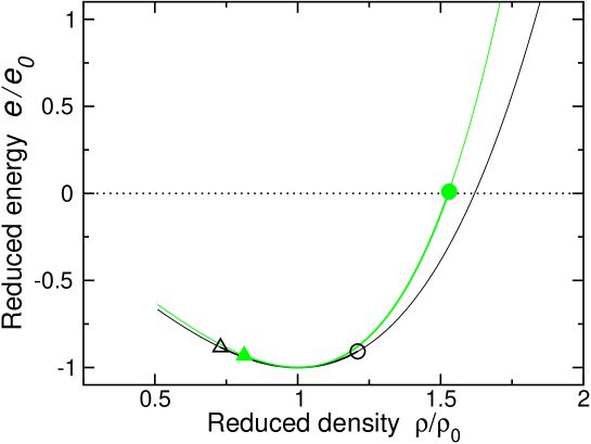
Figure 7.10: Comparison of the 2D and 3D equations of state. The thick lines are dmc results, while the thin lines are their extrapolations (7.21) to higher and lower densities. The triangles and circles denote the spinodal and freezing points, respectively. The black curves and empty symbols refer to the 3D data, while the green curves and filled symbols stand for the 2D data.

It is also remarkable the broader range of densities where helium remains liquid in 2D as compared to the 3D case, cf. Fig. 7.10.

The thickness of slabs in 3D is quite flat as a function of the inverse of the coverage $\widetilde{x}=L/N$ (cf. Fig. 4 in [Szy00]). This behavior contrasts with the 2D case where we observe a minimum in the $t(\widetilde{x})$ function (cf. Fig. 7.4). This discrepancy might just be due to a broader range of inverse converages explored in our work as compared with [Szy00]. In fact, our results are also quite flat in the region $\widetilde{x}\lesssim 2$, which relates to the larger slabs we have studied, $\rho_{c}/\rho_{0}\gtrsim 0.7$. Indeed, the calculations presented in [Szy00] are for slabs with $\rho_{c}/\rho_{0}^{3D}\gtrsim 0.6$. However, this does not rule out an influence of dimensionality on the behavior of the thickness, as is pointed out by the different values for the semi-infinite system: $t_{\rm semi}^{2D}\approx 11$ Å vs. $t_{\rm semi}^{3D}\approx 7$ Å.

7.5.2 2D clusters according to df and qmc calculations

Let us now turn to finite clusters and compare the results we have obtained by the dmc (Ch. 6) and df (this chapter) methods. First, let us look at the energy per particle, plotted in Fig. 7.5. We see that both calculations give very similar values for $N=121$, while for $N<121$ the df energies are always less bound than the dmc ones. On the other hand, there is a nice agreement of the mass formulas for $N\gtrsim 121$ ($z\lesssim 0.1$). This behavior is to be expected as the parameters defining the functional ($b,c,\gamma,d$) have been fixed so as to reproduce properties of the homogeneous and semi-infinite systems (see Sect. 7.2). For the same reason, the deviations for small clusters, where surface effects are most important, are not surprising. Indeed, from Fig. 7.6, we see that the density profile of the droplets does not present a truly ‘bulk’ region in its interior for clusters with less that 121 atoms. Nevertheless, the maximum relative deviation of the energy per particle is just around 15%.

In Fig. 7.11 we show the density profiles obtained in the vmc, dmc and df approaches for the $N=64$ drop, for which the energy calculated by the last two techniques is quite similar and the fluctuations in the dmc profile are small.

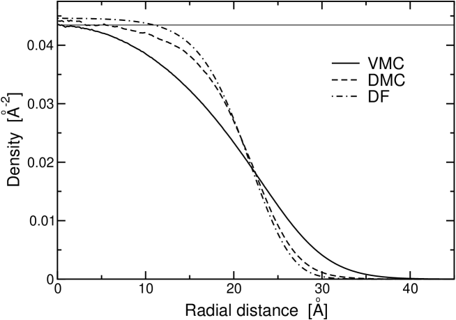
Figure 7.11: Density profiles of the $N=64$ cluster from the vmc (solid line), dmc (dashed line) and df (dash-dotted line) calculations. The thin horizontal line is the bulk saturation density.

In this comparison one can see that the df and dmc profiles are quite close to each other, with the surface location and thickness very similar as compared with the vmc ones. Thus, we can conclude that the description given by the zero-range Density Functional (7.3) is preferable over that of the simple vmc calculation. In this sense, it is worth mentioning that density profiles of 3D drops calculated with dmc and with finite-range density functionals show a similar agreement [BGH⁺06]. Indeed, the values for $R$ and $\langle r^{2}\rangle^{1/2}$ of the generalized Fermi-profile fits for the dmc and df data are in general in good agreement (cf. Tables 6.4 and 7.2). Even though a closer look at the data shows that $R$ in the dmc calculations is typically smaller than that from the df ones, the behavior of the rms radius is very much the same, with differences at most of 6%.

Regarding the thickness, one observes that it is quite constant for all df profiles, with a slowly decreasing behavior towards the value for the semi-infinite system, $t_{\rm semi}=11.03$ Å. This is in clear contrast with what happens with the dmc data, which are growing with $N$. In fact, the df thickness turns out to be systematically smaller than the dmc one, i. e., the df profiles present sharper surfaces than the dmc ones.

7.6 Summary and conclusions

We have constructed a density functional suitable to study non-homogeneous two-dimensional ⁴He systems. The parameters of the functional have been fixed by demanding it to reproduce some known properties of the homogeneous and semi-infinite systems. Then, we have considered two-dimensional slabs and analytically shown that the line tension extracted from a mass formula adapted to this type of geometry, is consistent with the value of the line tension of the semi-infinite system. We also observe that, as in three-dimensional slabs, the thickness and the central density of the slabs approach from below the values corresponding to the semi-infinite system, while the radius diverges.

We have also studied the energetics and structure of 2D clusters. In particular, clusters with a very large number of atoms have been used to study the behavior of the mass formula and to establish how the system approaches the bulk limit. The central density of the clusters when $N\rightarrow\infty$ approaches the saturation density from above and, therefore, the internal regions of the clusters are more compressed than the bulk system while the external regions have densities which would correspond to negative pressures or even below the spinodal point for a uniform system . This behavior reflects the existence of a tension on the boundary of the drop that keeps it bound.

The profiles of the clusters are very well fitted by a generalized Fermi function. The thickness of the cluster slowly approaches the thickness of the semi-infinite system, as it also happens in the case of the slab geometry, but in this case from above. This behavior contrasts with the dmc data, which were however obtained for quite small clusters, far from the bulk limit.

Finally, we have analyzed the linear behavior of the rms radius of the droplets in terms of $N^{1/2}$, and recovered the saturation density from the slope of this fit. We have also seen that the rms radii obtained from the df calculation are in very good agreement with the dmc results.

Altogether, we conclude that the proposed density functional is useful to perform reliable and computationally-affordable calculations for a variety of two-dimensional ⁴He systems and, in particular, for clusters where the number of particles is prohibitive for a Monte Carlo calculation.

Conclusions and future perspectives

Ars longa, beca brevis

Proverbium becarii

The purpose of this thesis has been the study of various atomic systems where the quantum effects are most visible, by means of a number of tools of many-body physics. In Chapter 1 we have presented in a general form the bcs theory of superconductivity for fermionic systems. We have made use of the well-known Green’s functions’ formalism to write the gap and number equations in a general form, capable of being used at zero and at finite temperature, both for density-symmetric and asymmetric systems. We have recovered the well-known result that the zero-temperature $s$-wave gap for the symmetric system in the weak-coupling limit has an exponential dependence on the interaction and the Fermi momentum, namely

$$\Delta_{\rm sym}=\frac{8}{e^{2}}\mu\exp\left(\frac{\pi}{2k_{F}a}\right)\qquad(a<0)\>.$$

The critical temperature for the superfluid transition has a similar behavior on the parameters of the system. One can write the corresponding result as

$$k_{B}T_{c}=\frac{e^{\gamma}}{\pi}\Delta_{\rm sym}\approx 0.567\Delta_{\rm sym}\>.$$

In Chapter 2 we have analyzed the prospect for $s$-wave pairing in the bcs framework for large density asymmetries. The main conclusions of this chapter are:

• The maximum asymmetry for which bcs pairing is possible is

  $$\alpha_{\rm max}^{BCS}\equiv\frac{\rho_{\uparrow}-\rho_{\downarrow}}{\rho_{\uparrow}+\rho_{\downarrow}}=\frac{3}{4}\frac{\Delta_{\rm sym}}{\mu}\>,$$

  which in the low-density limit is a very small quantity. We have checked numerically this prediction by solving self-consistently the gap and number equations; the agreement, as shown in Fig. 2.6, is remarkable for all $\alpha$.

• We have also checked numerically the dependence of the value of the gap with temperature for the symmetric system, and seen that it follows the expected limiting behaviors at low temperatures $T\ll T_{c}$ and close to the critical region $T\lesssim T_{c}$, cf. Fig. 2.4.

• Finally, we have analyzed the prospect for a bcs transition in $p$-wave between identical fermions, mediated by another fermionic species. For a density-symmetric system, the gap

  $$\frac{\Delta_{p\mbox{-}\rm wave}}{\mu}\propto\exp\left[-13\left(\frac{\pi}{2k_{F}a}\right)^{2}\right]\>,$$

  is very small, but it may be optimized by appropriately adjusting the density asymmetry. In practice, a sharp maximum appears for $\alpha_{\rm opt}\approx 0.478$.

In Chapter 3 we have studied two structures for the ground state alternative to the usual bcs one: the plane-wave loff and the dfs phases.

• As it is well-known, the loff phase can sustain pairing for larger asymmetries and has lower free energy than bcs. We have quantified this effect for the case of ⁶Li at ultralow temperatures and in the weak-coupling regime: we have shown that the loff phase if preferable to the bcs one for asymmetries $4\%\leq\alpha\leq 5.7\%$.

• The dfs phase consists in an ellipsoidal deformation of the Fermi surfaces of the two pairing species. More precisely, the surface of the most populated species becomes prolate (i. e., cigar-like) along a symmetry-breaking axis randomly chosen by the system. The surface of the less populated species becomes oblate (i. e., pancake-like), so that the two Fermi surfaces have, in the end, approached each other in the plane perpendicular to the symmetry-breaking axis. In this case, only rotational symmetry is broken.

• We have numerically evaluated the gap and free energy of the dfs phase, and we have shown that it becomes the ground state for the ⁶Li system under study for asymmetries $\alpha\gtrsim 4\%$.

• We have proposed an easy scheme of detecting the dfs phase by means of a time-of-flight determination of the momentum distribution for an atomic gas confined in a spherical trap.

It is our purpose to analyze in the future the excitation spectrum of the dfs state, to identify the new Goldstone mode that shold appear due to the breaking of rotational symmetry. One should also remember that more general structures for the loff phase are possible, which could qualitatively modify our conclusions.

In Chapter 4 we have considered the effects of the presence of a bosonic species in a single-component fermionic system.

• For the three-dimensional case, the induced pairing is optimized for a bosonic density

  $$\rho_{B}=\frac{\rho_{F}^{2/3}}{2.88a_{BB}}\>,$$

  where $a_{BB}$ is the $s$-wave scattering length for boson-boson collisions.

• For the two-dimensional case, the logarithmic dependence of the transition matrix on the collision energy requires a more delicate treatment, and the value of the optimal densities depends on the parameters determining the collision properties among bosons, $E_{BB}$, and between bosons and fermions, $E_{BF}$. We have shown that, for the case that both species have similar masses, $E_{BB}$ plays only a minor role, and the optimal density ratio is given by

  $$\left.\frac{\rho_{B}}{\rho_{F}}\right|_{\rm opt} =-0.59\left[\ln\zeta-0.35\right]\>,$$

  $$\zeta(\varepsilon_{F}) :=\frac{m_{F}}{m_{B}}\frac{\varepsilon_{F}}{E_{BB}}\>.$$

  Under these conditions, energy gaps of the order of the fermion chemical potential may be achieved.

• For the case of trapped, quasi-two-dimensional atomic systems, this regime seems to be achievable for mixtures with attractive interspecies interaction $a_{BF}<0$ such as ⁸⁷Rb-⁴⁰K. On the other hand, for $a_{BF}>0$ (as in the ⁷Li-⁶Li mixtures) one should also analyze the stability of the system.

In Chapter 5 we have studied the real-time evolution of a Bose-Einstein condensate with spin degree of freedom. We have recalled that, for the case of spin $f=1$, two possible ground-state structures are possible

• ‘Ferromagnetic’: when the coupling constant in the collision channel with total spin $F=2$ is attractive, $c_{2}<0$, the spin tends to be locally maximized. This translates into a mixture of all spin components in each point.

• ‘Antiferromagnetic’: when $c_{2}>0$, the ground state is realized by minimizing the expectation value of the spin. As a consequence, atoms with spin projection $m=\pm 1$ will tend to repel $m=0$ atoms.

The dynamical evolution in the first case, which is realized for ⁸⁷Rb atoms in their electronic ground state, presents these characteristics:

• It shows oscillations in the populations of the various hyperfine states $m=1,0,-1$. At zero temperature, and for an initial state with zero magnetizaton, these oscillations are around the ground-state configuration $(25\%,50\%,25\%)$. At a finite temperature $T=0.2T_{c}$, which we simulate via the inclusion of phase fluctuations, all components are equally populated after a fast damping process.

• The density profiles feature small spin domains of a characteristic size $l_{\rm dom}\sim 10\leavevmode\nobreak\ \mu$m, that appear after $\sim$100 ms. This domain formation may be interpreted as the consequence of a dynamical instability of the spin excitation modes of the ‘ferromagnetic’ system. At zero temperature, the domains formed by $m=\pm 1$ atoms overlap, thus conserving locally the initial magnetization. At finite temperature, the symmetry between $m=1$ and $m=-1$ is broken by the fluctuating phases, and different, interpenetrating domains of all components appear. In this case, the formation of domains is much faster: it occurs for times $\sim$10 ms.

We have also analyzed a case with ‘antiferromagnetic’ interactions for which:

• The population oscillations are almost coherent at zero temperature, but present a very small relaxing behavior at finite temperature.

• The density profiles barely evolve at $T=0.2T_{c}$, while at zero temperature Josephson-like oscillations may be identified.

For the future, we plan studies on the role of the initial conditions and on effects of temperature and external magnetic fields. Also the study of condensates with higher spin values (in particular, $f=2$) is interesting in order to interpret a number of experimental results.

In the second part of the thesis, we have presented two microscopic studies on ⁴He systems in two dimensions. In Chapter 6 we have performed both Variational and Diffusion Monte Carlo calculations for finite clusters. First we have built a good variational function by including Jastrow-like correlations together with a Gaussian term to take into account the self-binding of the drops. This function has then been used as importance function for the dmc calculation. The main conclusions that we get from these studies are:

• From the results for the energy per particle as a function of the number of atoms in the drop, we have constructed a mass formula,

  $$\frac{E}{N}=\varepsilon_{b}+\frac{\varepsilon_{l}}{N^{1/2}}+\frac{\varepsilon_{c}}{N}\>.$$

  The first coefficient coincides with the calculated value for the energy per particle at saturation of the homogeneous system. From $\varepsilon_{l}$ we have extracted a value for the line energy due to the finite character of these systems,

  $$\lambda_{\rm DMC}=0.121\mbox{\leavevmode\nobreak\ K/\AA}\>,$$

  which is the principal result of this chapter.

• We have also analyzed the density profiles obtained by the forward walking method to evaluate pure estimators. The profiles can be very well fitted to a generalized Fermi function, and provide an alternative determination for the bulk saturation density, which roughly coincides with the value from dmc calculations.

In Chapter 7 we have used the previous results for the homogenous system and the line tension to build a zero-range density functional, with an energy density of the form

$$\varepsilon[\rho]=\frac{\hbar^{2}}{2m}\frac{|\nabla\rho|^{2}}{4\rho}+b\rho^{2}+c\rho^{2+\gamma}+d|\nabla\rho|^{2}\>.$$

The parameters $\{b,c,\gamma\}$ have been fixed so as to reproduce the energy per particle, density and speed of sound at saturation, while $d$ has been determined by demanding that the line tension of the semi-infinite system equals $\lambda_{\rm DMC}$. The conclusions that we draw from the subsequent analysis are:

• The energy per particle of two-dimensional slabs approaches that of the bulk system slowly, in a linear way. In this limit the radius of the slabs diverges as expected. Other physical parameters approach the corresponding bulk values much faster. For instance, the chemical potential or the thickness have attained their bulk values for inverse coverages $\widetilde{x}\approx 1$ Å^-1.

• For clusters, the bulk limit is harder to attain, and both the energy and the chemical potential approach linearly the corresponding limiting values. An analysis of the energy per particle in the form of a mass formula gives a positive value for the curvature term $\varepsilon_{c}$, as one expects from the lack of binding energy of the atoms on the surface.

• Some features of the density profiles of finite clusters are similar to their three-dimensional counterparts. For example, the central density presents a ‘leptodermous’ behavior, approaching the bulk saturation density from above.

• Finally, an analysis of these profiles in terms of hydrodynamical equilibrium has shown that near the surface of the puddles the pressure presents a dip down to negative values. This has been interpreted as the effect of the line tension. Hydrodynamic equilibrium demands de presence of a force (due to the He-He interaction) that close to the surface is proportional to the distance to it.

Further studies to be performed on ⁴He systems are the calculation of the natural orbits and the subsequent evaluation of the condensate fraction.

Vale.

Appendix A Summing up over fermionic Matsubara frequencies

In this appendix we show how to evaluate a summation over Matsubara frequencies. First of all, let us shortly introduce the Matsubara technique for finite-temperature Green’s functions (see [Mat92]).

At zero temperature, the solution of the Schrödinger equation

$$i\hbar\frac{\partial}{\partial t}\psi(\bm{x},t)=\hat{H}\psi(\bm{x},t)$$ (A.1)

can be reexpressed in terms of the (zero temperature) Green’s function (or propagator)

$$G^{T=0}(\bm{x},t;\bm{x^{\prime}},t^{\prime}):=-i\left\langle\Psi_{0}\left|T\left[\hat{\psi}(\bm{x},t)\hat{\psi}^{\dagger}(\bm{x^{\prime}},t^{\prime})\right]\right|\Psi_{0}\right\rangle\>,$$ (A.2)

where $T$ is the time ordering operator,

$$T[\hat{a}(t)\hat{b}(t^{\prime})]=\hat{a}(t)\hat{b}(t^{\prime})\Theta(t-t^{\prime})\pm\hat{b}(t^{\prime})\hat{a}(t)\Theta(t^{\prime}-t)\>,$$

and $|\Psi_{0}\rangle$ is the exact ground state of the sytem. The operators in (A.2) are defined int the Heisenberg picture as

$${\cal\hat{O}}(t):=e^{it\hat{H}}{\cal\hat{O}}e^{-it\hat{H}}\>.$$

Analogously, for a system at $T>0$, we define a propagator as a thermal average of the same operator as before:

$$G^{T}(\bm{x},t;\bm{x^{\prime}},t^{\prime}):=-i\left\langle T\left[\hat{\psi}(\bm{x},t)\hat{\psi}^{\dagger}(\bm{x^{\prime}},t^{\prime})\right]\right\rangle$$ (A.3)

where the angular brackets stand for the thermal average with the statistical operator $\rho^{T}=\exp[-\beta(\hat{H}-\mu\hat{N})]$,

$$\left\langle{\cal O}\right\rangle:=\frac{{\rm Tr}\left[\rho^{T}{\cal O}\right]}{\cal Z}\>,\qquad{\cal Z}={\rm Tr}\left[\rho^{T}\right]\>.$$

However, the statistical operator satisfies Bloch’s equation, namely

$$-\frac{\partial\rho}{\partial\beta}=\left({\hat{H}}-\mu\hat{N}\right)\rho\>,$$

which is formaly identical to Schrödinger’s equation with the equivalences

$$it/\hbar\leftrightarrow\beta\qquad\hat{H}\leftrightarrow\hat{H}-\mu\hat{N}\>.$$

This suggests to define the finite-temperature Green’s function just as the zero-temperature one, but performing these replacements everywhere, that is,

$$G(\bm{x}\tau,\bm{x^{\prime}}\tau^{\prime}):=-\left\langle T\left[\hat{\psi}(\bm{x}\tau)\hat{\psi}^{\dagger}(\bm{x^{\prime}}\tau^{\prime})\right]\right\rangle\>,$$ (A.4)

with $\tau=it$ the so-called “imaginary time”. It can be shown that this propagator (and not the $G^{T}$ defined above) can be evaluated in a series expansion as it can be done with the zero-temperature Green’s function.

We turn now to show three general properties of this $G$ that will be of interest. Dropping for simplicity the $\bm{x}$-dependence of the propagator, it is easy to show that $G(\tau,\tau^{\prime})=G(\tau^{\prime}-\tau)$:

$$G(\tau,\tau^{\prime}) =-\frac{1}{{\cal Z}}{\rm Tr}\left[e^{-\beta K}e^{K\tau/\hbar}\hat{\psi}e^{-K\tau/\hbar}e^{K\tau^{\prime}/\hbar}\hat{\psi}^{\dagger}e^{-K\tau^{\prime}/\hbar}\right]$$

$$=-\frac{1}{{\cal Z}}{\rm Tr}\left[e^{K\tau/\hbar}e^{-\beta K}\hat{\psi}e^{K(\tau^{\prime}-\tau)/\hbar}\hat{\psi}^{\dagger}e^{-K\tau^{\prime}/\hbar}\right]$$

$$=-\frac{1}{{\cal Z}}{\rm Tr}\left[e^{-\beta K}\hat{\psi}e^{K(\tau^{\prime}-\tau)/\hbar}\hat{\psi}^{\dagger}e^{-K(\tau^{\prime}-\tau)/\hbar}\right]\equiv G(0,\tau^{\prime}-\tau)\>,$$

where we introduced the grand-canonical Hamiltonian $K=\hat{H}-\mu\hat{N}$, and used the cyclic property of the trace.

We can also show that, for fermion, $G(-\beta\hbar)=-G(0)$:

$$G(-\beta\hbar) =-\frac{1}{{\cal Z}}{\rm Tr}\left[e^{-\beta K}\hat{\psi}e^{-K\beta}\hat{\psi}^{\dagger}e^{K\beta}\right]=-\frac{1}{{\cal Z}}{\rm Tr}\left[e^{-\beta K}\hat{\psi}^{\dagger}e^{K\beta}e^{-K\beta}\hat{\psi}\right]$$

$$=-\frac{1}{{\cal Z}}{\rm Tr}\left[e^{-\beta K}\hat{\psi}^{\dagger}\hat{\psi}\right]=\pm G(0)\>,$$

where we used again the cyclic property of the trace.

With these two properties, it is easy to show that $G(\tau)$ is periodic with period $\beta\hbar$, and it is useful to introduce its components in Fourier space,

$$G(\tau)=\frac{1}{\beta\hbar}\sum_{n}e^{-i\omega_{n}\tau}G(\omega_{n})\>.$$ (A.5)

Then, we have

$$G(0)=\frac{1}{\beta\hbar}\sum_{n}G(\omega_{n})\qquad G(-\beta\hbar)=\frac{1}{\beta\hbar}\sum_{n}e^{i\hbar\omega_{n}\beta}G(\omega_{n})\>.$$

From the condition $G(-\beta\hbar)=-G(0)$ we therefore get

$$e^{i\hbar\omega_{n}\beta}=-1\Rightarrow\omega_{n}=(2n+1)\frac{\pi}{\beta\hbar}\>,$$ (A.6)

which are called fermionic Matsubara frequencies.

Let us return to the evaluation of a summation over such Matsubara frequencies $\omega_{n}$ as the one we encountered in Sect. 1.2.3, evaluation of

$$S=\sum_{n}\left(\frac{1}{i\hbar\omega_{n}-E_{k}}-\frac{1}{i\hbar\omega_{n}+E_{k}}\right)\;.$$ (A.7)

The way to perform this kind of sumations is to convert them by means of Cauchy’s theorem on integrals on the complex plane [Arf95]:

$$\frac{1}{2\pi i}\oint_{C}dzf(z)=\sum_{n}\mathrm{Res}\{f(z_{n})\}\;,$$ (A.8)

where $f(z)$ is an analytic function inside the region enclosed (in the mathematically positive sense) by the contour $C$ (see Fig.A.1) except on the points $\{z_{n}\}$, that are the poles of $f$; $\mathrm{Res}\{f(z_{n})\}$ is the residue of $f$ at $z_{n}$.

Looking at Eq. (A.7), we define a function $f$ on the complex plane by

$$f(z):=\frac{1}{z-\frac{\beta}{2}E_{k}}-\frac{1}{z+\frac{\beta}{2}E_{k}}\;,$$ (A.9)

so that now

$$S=\frac{\beta}{2}\sum_{n}f(z_{n})\;,\qquad z_{n}=\frac{\beta\hbar\omega_{n}}{2}i=\frac{2n+1}{2}\pi i\;.$$ (A.10)

It turns out that $\tanh(z)$ has poles precisely at the points $z=z_{n}$, and these poles have unit residues. Therefore, $f(z)\tanh(z)$ will have poles at the desired positions and with the desired residues, and can write

$$S=\frac{\beta}{2}\frac{1}{2\pi i}\oint_{C}dzf(z)\tanh(z)\;,$$ (A.11)

where the contour $C$ encloses the imaginary axis, as shown by the dashed line in Fig. A.1, but not the poles of $f$ on the real axis.

If we deform $C$ into $C^{\prime}+\Gamma$ (see again Fig. A.1), and realize that the integral over $\Gamma$ will not contribute at $|z|\rightarrow\infty$ because in that limit $f(z)\propto z^{-2}$, we get

$$S =\frac{\beta}{2}\frac{1}{2\pi i}\oint_{C^{\prime}+\Gamma}dzf(z)\tanh(z)=\frac{\beta}{2}\frac{1}{2\pi i}\oint_{C^{\prime}}dzf(z)\tanh(z)$$

$$=\frac{\beta}{2}\frac{1}{2\pi i}\left(-2\pi i\right)\sum_{z=\pm\frac{\beta}{2}E_{k}}\mathrm{Res}\{\tanh(z)\}=-\beta\tanh\left(\beta\frac{E_{k}}{2}\right)\;,$$ (A.12)

where we evaluated the integration over $C^{\prime}$ using again Cauchy’s theorem but now with a ‘$-$’ sign because $C^{\prime}$ is oriented in the mathematically negative sense, and we used the fact that $f(z)\tanh(z)$ is analytic on the real axis except at $z=\pm\beta E_{k}/2$. Thus, we obtain

$$\sum_{n}\left(\frac{1}{i\hbar\omega_{n}-E_{k}}-\frac{1}{i\hbar\omega_{n}+E_{k}}\right)=-\beta\tanh\left(\beta\frac{E_{k}}{2}\right)\;,$$ (A.13)

which is the result used in deriving Eqs. (1.23) and (2.1).

Figure A.1: Complex $z$-plane with the contours $C$ and $C^{\prime}+\Gamma$. The crosses indicate the poles of $\tanh(z)$ while the circles are located at $\pm E_{k}$.

Appendix B Deduction of the equations of motion of spin-$f$ condensates

B.1 Introduction

Consider the interaction between two spin-$f$ atoms:

$$V(\bm{r}_{1}-\bm{r}_{2}) =\delta(\bm{r}_{1}-\bm{r}_{2})\sum_{F=0}^{2f}g_{F}P_{F}$$ (B.1)

$$g_{F} =\frac{4\pi\hbar^{2}a_{F}}{M}$$ (B.2)

where $a_{F}$ is the $s$-wave scattering length in the channel of total spin $F$, and $M$ is the mass of the atoms. For bosons, only even $F$’s are allowed; for fermions, only odd $F$’s. From now on we shall consider only bosons. For example, for $f=1,2$, we have

$$V =g_{2}P_{2}+g_{0}P_{0} (f=1)$$

$$V =g_{4}P_{4}+g_{2}P_{2}+g_{0}P_{0} (f=2)$$

On the other hand, we also have:

$$\bm{f}_{1}\cdot\bm{f}_{2} =\sum_{F=0}^{2f}\lambda_{F}P_{F}$$ (B.3)

$$\lambda_{F} =\frac{F(F+1)-2f(f+1)}{2}$$ (B.4)

To show this, consider the addition of two spins $f$ to a total spin $F$:

$$(\bm{f}_{1}+\bm{f}_{2})^{2} =\bm{f}_{1}^{2}+\bm{f}_{2}^{2}+2\bm{f}_{1}\cdot\bm{f}_{2}=2f(f+1)+2\bm{f}_{1}\cdot\bm{f}_{2}$$

$$(\bm{f}_{1}+\bm{f}_{2})^{2} =F(F+1)$$

Therefore,

$$\bm{f}_{1}\cdot\bm{f}_{2}=\frac{F(F+1)-2f(f+1)}{2}\>.$$

To take into account all possible channels ($F=0,...,2f$) we must sum over $F$, projecting each contribution with the corresponding projector $P_{F}$, that is

$$\bm{f}_{1}\cdot\bm{f}_{2}=\sum_{F=0}^{2f}\frac{F(F+1)-2f(f+1)}{2}P_{F}\>.$$ (B.5)

For instance,

$$\bm{f}_{1}\cdot\bm{f}_{2} =-2P_{0}+P_{2} (f=1)$$

$$\bm{f}_{1}\cdot\bm{f}_{2} =-6P_{0}-3P_{2}+4P_{4} (f=2)$$

Finally, the normalization condition on the projectors provides the identity

$$\sum_{F=0}^{2f}P_{F}=1\>.$$ (B.6)

From all these equations we can obtain:

• Spin $f=1$:

  $$V =g_{2}P_{2}+g_{0}P_{0}$$

  $$\bm{f}_{1}\cdot\bm{f}_{2} =-2P_{0}+P_{2}$$

  $$P_{0}+P_{2} =1$$

  Therefore,

  $$V=\frac{2g_{2}+g_{0}}{3}+\frac{g_{2}-g_{0}}{3}\bm{f}_{1}\cdot\bm{f}_{2}\equiv c_{0}+c_{2}\bm{f}_{1}\cdot\bm{f}_{2}\>.$$

• Spin $f=2$:

  $$V =g_{4}P_{4}+g_{2}P_{2}+g_{0}P_{0}$$

  $$\bm{f}_{1}\cdot\bm{f}_{2} =-6P_{0}-3P_{2}+4P_{4}$$

  $$P_{0}+P_{2}+P_{4} =1$$

  Therefore,

  $$V=\frac{3g_{4}+4g_{2}}{7}+\frac{3g_{4}-10g_{2}+7g_{0}}{7}P_{0}+\frac{g_{4}-g_{2}}{7}\bm{f}_{1}\cdot\bm{f}_{2}\equiv c_{0}+c_{1}P_{0}+c_{2}\bm{f}_{1}\cdot\bm{f}_{2}\>.$$

Thus, we can write the Hamiltonian in the form

$$H-\mu N =\sum_{a=-f}^{f}\int\mathrm{d}^{3}r\left\{\hat{\psi}^{+}_{a}\left(-\frac{\hbar^{2}}{2m}\nabla^{2}\right)\hat{\psi}_{a}+(V_{\rm ext}-\mu)\hat{\psi}^{+}_{a}\hat{\psi}_{a}\right.$$

$$+\sum_{a^{\prime}=-f}^{f}\frac{1}{2}c_{0}\hat{\psi}^{+}_{a}\hat{\psi}^{+}_{a^{\prime}}\hat{\psi}_{a^{\prime}}\hat{\psi}_{a}+\sum_{a^{\prime},b,b^{\prime}=-f}^{f}\frac{1}{2}c_{2}\hat{\psi}^{+}_{a}\hat{\psi}^{+}_{a^{\prime}}\bm{f}_{ab}\cdot\bm{f}_{a^{\prime}b^{\prime}}\hat{\psi}_{b^{\prime}}\hat{\psi}_{b}$$

$$+\sum_{a^{\prime},b,b^{\prime}=-f}^{f}\frac{1}{2}c_{1}\hat{\psi}^{+}_{a}\hat{\psi}^{+}_{a^{\prime}}(P_{0})_{aa^{\prime},bb^{\prime}}\hat{\psi}_{b^{\prime}}\hat{\psi}_{b}\mbox{\leavevmode\nobreak\ \leavevmode\nobreak\ [this term only for $f=2$]}$$

$$\left.-\sum_{a^{\prime}=-f}^{f}p(z)\hat{\psi}^{+}_{a}(F_{z})_{aa^{\prime}}\hat{\psi}_{a^{\prime}}+\sum_{a^{\prime}=-f}^{f}q\hat{\psi}^{+}_{a}(F^{2}_{z})_{aa^{\prime}}\hat{\psi}_{a^{\prime}}\>,\right\}$$ (B.7)

where $\hat{\psi}_{a}$ is the anihilation operator for an atom in state $|1,a\rangle$, Notice also that we have taken into account the effect of a magnetic field in the lowest two orders by

$$p(z) =g\mu_{B}B(z)\mbox{\leavevmode\nobreak\ \leavevmode\nobreak\ \leavevmode\nobreak\ \leavevmode\nobreak\ \leavevmode\nobreak\ \leavevmode\nobreak\ \leavevmode\nobreak\ linear Zeeman effect for $\vec{B}=B\hat{z}$,}$$

$$q =\frac{g^{2}\mu_{B}^{2}}{16h\nu_{hfs}}B_{0}^{2}\mbox{\leavevmode\nobreak\ \leavevmode\nobreak\ \leavevmode\nobreak\ \leavevmode\nobreak\ quadratic Zeeman effect}\>.$$

Here $g$ is the gyromagnetic factor for the atom, and $h\nu_{hfs}$ is the hyperfine splitting characteristic of the manifold in which the atoms are.

B.2 Mean-field dynamical equations for a spin-1 condensate

We make the usual mean-field approximation for the field operators,

$$\psi_{a}(\bm{r})=\langle\hat{\psi}_{a}(\bm{r})\rangle\>,$$ (B.8)

The equation of motion for the field $\psi_{m}$ can be derived from the Hamiltonia by functional differentiation:

$$i\hbar\frac{\partial\psi_{m}}{\partial t} =\frac{\delta(H-\mu N)}{\delta\psi^{+}_{m}}$$

$$=-\frac{\hbar^{2}}{2M}\nabla^{2}\psi_{m}+[V_{\rm ext}-\mu]\psi_{m}$$

$$+c_{0}\left(\sum_{a}\psi^{*}_{a}\psi_{a}\right)\psi_{m}+c_{2}\left(\sum_{ab}\psi^{*}_{a}\bm{f}_{ab}\psi_{b}\right)\cdot\left(\bm{f}\psi\right)_{m}$$

$$-p(z)\left(F_{z}\psi\right)_{m}+q\left(F_{z}^{2}\psi\right)_{m}\>.$$ (B.9)

In the mean field approximation, one can rewrite the several terms in this way:

• $\sum_{a}\psi^{*}_{a}\psi_{a}$:

  $$\sum_{a}\psi^{*}_{a}\psi_{a}\rightarrow\sum_{a}n_{a}(\bm{r})=n(\bm{r})\>,$$

  which is the total density of particles at point $\bm{r}$.

• $\sum_{ab}\psi^{+}_{a}\bm{f}_{ab}\psi_{b}$:

  $$\sum_{ab}\psi^{+}_{a}\bm{f}_{ab}\psi_{b} \rightarrow\sum_{ab}\sum_{i=x,y,z}\psi^{*}_{a}\left(F_{i}\right)_{ab}\psi_{b}\hat{\imath}$$

  $$=\sum_{i}\hat{\imath}\left\{\left(F\right)_{11}|\psi_{1}|^{2}+\left(F\right)_{10}\psi^{*}_{1}\psi_{0}\left(F\right)_{1-1}\psi^{*}_{1}\psi_{-1}+\cdots\right\}$$

  $$=\left(\begin{array}[]{cc}[i=x]&\frac{1}{\sqrt{2}}\left\{\psi^{*}_{1}\psi_{0}+\psi^{*}_{0}\psi_{1}+\psi^{*}_{0}\psi_{-1}+\psi^{*}_{-1}\psi_{0}\right\}\cr[i=y]&\frac{1}{i\sqrt{2}}\left\{\psi^{*}_{1}\psi_{0}-\psi^{*}_{0}\psi_{1}+\psi^{*}_{0}\psi_{-1}-\psi^{*}_{-1}\psi_{0}\right\}\cr[i=z]&\left\{n_{1}-n_{-1}\right\}\end{array}\right)\>,$$

  where we have used the matrix expression of the spin operators, i. e. the Pauli matrices for spin $f=1$, namely

  $$F_{x} =\frac{1}{\sqrt{2}}\left(\begin{array}[]{ccc}0&1&0\\ 1&0&1\\ 0&1&0\\ \end{array}\right)\>,$$ (B.10d)

  $$F_{y} =\frac{1}{i\sqrt{2}}\left(\begin{array}[]{ccc}0&1&0\\ -1&0&1\\ 0&-1&0\\ \end{array}\right)\>,$$ (B.10h)

  $$F_{z} =\left(\begin{array}[]{ccc}1&0&0\\ 0&0&0\\ 0&0&-1\\ \end{array}\right)\>.$$ (B.10l)

• $\langle\bm{f}\rangle\cdot\left(\bm{f}\psi\right)_{m}$: As above, we use the Pauli matrices to arrive at

  $$\left(\sum_{ab}\psi^{*}_{a}\bm{f}_{ab}\psi_{b}\right)\cdot\left(\bm{f}\psi\right)_{m}=\left(\begin{array}[]{cc}[m=1]&\psi_{0}^{2}\psi^{*}_{-1}+(n_{1}+n_{0}-n_{-1})\psi_{1}\cr[m=0]&(n_{1}+n_{-1})\psi_{0}+2\psi_{1}\psi^{*}_{0}\psi_{-1}\cr[m=-1]&\psi_{0}^{2}\psi^{*}_{1}+(n_{-1}+n_{0}-n_{1})\psi_{-1}\end{array}\right)$$

Collecting the partial results, we get

$$i\hbar\frac{\partial\psi_{1}}{\partial t} =\left[-\frac{\hbar^{2}}{2M}\nabla^{2}+V_{\rm ext}+c_{0}n(\bm{r})\right]\psi_{1}$$

$$+c_{2}\left[\left(n_{1}+n_{0}-n_{-1}\right)\psi_{1}+\psi^{2}_{0}\psi^{*}_{-1}\right]$$

$$-p\psi_{1}+q\psi_{1}$$ (B.11a)

$$i\hbar\frac{\partial\psi_{0}}{\partial t} =\left[-\frac{\hbar^{2}}{2M}\nabla^{2}+V_{\rm ext}+c_{0}n(\bm{r})\right]\psi_{0}$$

$$+c_{2}\left[\left(n_{1}+n_{-1}\right)\psi_{0}+2\psi_{1}\psi^{*}_{0}\psi_{-1}\right]$$ (B.11b)

$$i\hbar\frac{\partial\psi_{-1}}{\partial t} =\left[-\frac{\hbar^{2}}{2M}\nabla^{2}+V_{\rm ext}+c_{0}n(\bm{r})\right]\psi_{-1}$$

$$+c_{2}\left[\left(n_{-1}+n_{0}-n_{1}\right)\psi_{-1}+\psi^{2}_{0}\psi^{*}_{1}\right]$$

$$+p\psi_{-1}+q\psi_{-1}\>.$$ (B.11c)

We have separated in different lines the contributions: (1) equal for all components, (2) proportional to $c_{2}$ and related to spin-exchange collisions, and (3) terms due to the presence of a magnetic field. Note that, except for the linear Zeeman term ($\propto p\propto B$), the equations for $m=1$ and $m=-1$ are invariant under the relabelling $1\leftrightarrow-1$, indicating our freedom to choose the orientation of the quantization axis. More generally, the equations are invariant under the time-reversal operator, that transforms $1\leftrightarrow-1$ and $B\rightarrow-B$.

These dynamical equations can be written in the shorter form (5.7) by introducing effective potentials that, in the case of a non-vanishing magnetic field, read

$$V^{\mathrm{eff}}_{\pm 1} =V_{\mathrm{ext}}+c_{0}n+c_{2}(\pm n_{1}+n_{0}\mp n_{-1})\mp p+q$$

$$V^{\mathrm{eff}}_{0} =V_{\mathrm{ext}}+c_{0}n+c_{2}(n_{1}+n_{-1})\>.$$

It is also possible to derive a set of coupled continuity equations from (B.11). To this end, we define the number density of the $m$ component as usual by

$$n_{m}(\bm{r},t) =|\psi_{m}(\bm{r},t)|^{2}\>.$$

Applying the operator $i\hbar\partial/\partial t$ to $n_{0}$, we get

$$i\hbar\frac{\partial n_{0}}{\partial t} =i\hbar\frac{\partial\psi_{0}^{*}}{\partial t}\psi_{0}+i\hbar\frac{\partial\psi_{0}}{\partial t}\psi_{0}^{*}$$

$$=-\frac{\hbar^{2}}{2M}\left[-\psi_{0}\nabla^{2}\psi_{0}^{*}+\psi_{0}^{*}\nabla^{2}\psi_{0}\right]+2c_{2}\left[-\psi_{1}^{*}\psi_{0}^{2}\psi_{-1}^{*}+\psi_{1}(\psi_{0}^{2})^{*}\psi_{-1}\right]\>.$$

Now, defining the quantum current of the $m$ component by

$$\bm{j}_{m}=\frac{\hbar}{2iM}(\psi_{m}^{*}{\bm{\nabla}}\psi_{m}-\psi_{m}{\bm{\nabla}}\psi_{m}^{*})\>,$$

we can rewrite this result as

$$\frac{\partial n_{0}}{\partial t}+\bm{\nabla}\cdot\bm{j}_{0} =2\frac{c_{2}}{i\hbar}\left[-\psi_{1}^{*}\psi_{0}^{2}\psi_{-1}^{*}+\psi_{1}(\psi_{0}^{2})^{*}\psi_{-1}\right]\>,$$

which has the form of a continuity equation with a source term given by $-(2c_{2}/\hbar)\,\mbox{Im}[T_{0}\psi_{0}]\in\mathbb{R}$, with $T_{0}:=2\psi_{1}\psi_{0}^{*}\psi_{-1}$. For the $m=\pm 1$ components, a similar treatment yields

$$\frac{\partial n_{\pm 1}}{\partial t}+\bm{\nabla}\cdot\bm{j}_{\pm 1} =-\frac{2c_{2}}{\hbar}\,\mbox{Im}[T_{\pm 1}\psi_{\pm 1}]\>,$$

$$T_{\pm 1}^{*} :=\psi_{0}^{2}\psi_{\mp 1}^{*}\>.$$

B.3 Mean-field dynamical equations for a spin-2 condensate

The starting point is the grand-canonical Hamiltonian that, for $f=2$ reads:

$$H-\mu N =\sum_{a=-2}^{2}\int\mathrm{d}^{3}r\left\{\psi^{\dagger}_{a}\left(-\frac{\hbar^{2}}{2M}\nabla^{2}\right)\psi_{a}+(V_{\rm ext}-\mu)\psi^{+}_{a}\psi_{a}\right.$$

$$+\sum_{a^{\prime}=-2}^{2}\frac{1}{2}c_{0}\psi^{+}_{a}\psi^{+}_{a^{\prime}}\psi_{a^{\prime}}\psi_{a}+\sum_{a^{\prime},b,b^{\prime}=-2}^{2}\frac{1}{2}c_{2}\psi^{+}_{a}\psi^{+}_{a^{\prime}}\bm{f}_{ab}\cdot\bm{f}_{a^{\prime}b^{\prime}}\psi_{b^{\prime}}\psi_{b}$$

$$+\sum_{a^{\prime},b,b^{\prime}=-2}^{2}\frac{1}{2}c_{1}\psi^{+}_{a}\psi^{+}_{a^{\prime}}(P_{0})_{aa^{\prime},bb^{\prime}}\psi_{b^{\prime}}\psi_{b}$$

$$\left.-\sum_{a^{\prime}=-2}^{2}p(z)\psi^{+}_{a}(F_{z})_{aa^{\prime}}\psi_{a^{\prime}}+\sum_{a^{\prime}=-2}^{2}q\psi^{+}_{a}(F^{2}_{z})_{aa^{\prime}}\psi_{a^{\prime}}\>,\right\}$$ (B.12)

$$\langle\langle\hat{A}\rangle\rangle :=\sum_{a,a^{\prime},b,b^{\prime}}\xi^{*}_{a}\xi^{*}_{a^{\prime}}A_{ab}\xi_{b^{\prime}}\xi_{b}\>,\quad A_{aa^{\prime},bb^{\prime}}:=\langle aa^{\prime}|\hat{A}|bb^{\prime}\rangle$$ (B.13)

Again, we derive the equations of motion of the field operators by a functional derivative of the Hamiltonian (B.12):

$$i\hbar\frac{\partial\psi_{m}}{\partial t} =\frac{\delta(H-\mu N)}{\delta\psi^{+}_{m}}$$

$$=-\frac{\hbar^{2}}{2M}\nabla^{2}\psi_{m}+[V_{\rm ext}-\mu]\psi_{m}$$

$$+c_{0}\left(\sum_{a}\psi^{\dagger}_{a}\psi_{a}\right)\psi_{m}+c_{2}\left(\sum_{ab}\psi^{\dagger}_{a}\bm{f}_{ab}\psi_{b}\right)\cdot\left(\bm{f}\psi\right)_{m}$$

$$+c_{1}\sum_{abc}\psi^{\dagger}_{a}\left(P_{0}\right)_{ma,bc}\psi_{c}\psi_{b}$$

$$-p(z)\left(F_{z}\psi\right)_{m}+q\left(F_{z}^{2}\psi\right)_{m}\>.$$ (B.14)

As we are working with $f=2$, all spin operators can be represented by the following $5\times 5$ Pauli matrices:

$$F_{x} =\left(\begin{array}[]{ccccc}0&1&0&0&0\\ 1&0&\sqrt{\frac{3}{2}}&0&0\\ 0&\sqrt{\frac{3}{2}}&0&\sqrt{\frac{3}{2}}&0\\ 0&0&\sqrt{\frac{3}{2}}&0&1\\ 0&0&0&1&0\\ \end{array}\right)\>,$$ (B.15f)

$$F_{y} =-i\left(\begin{array}[]{ccccc}0&1&0&0&0\\ -1&0&\sqrt{\frac{3}{2}}&0&0\\ 0&-\sqrt{\frac{3}{2}}&0&\sqrt{\frac{3}{2}}&0\\ 0&0&-\sqrt{\frac{3}{2}}&0&1\\ 0&0&0&-1&0\\ \end{array}\right)\>,$$ (B.15l)

$$F_{z} =\left(\begin{array}[]{ccccc}2&0&0&0&0\\ 0&1&0&0&0\\ 0&0&0&0&0\\ 0&0&0&-1&0\\ 0&0&0&0&-2\\ \end{array}\right)\>.$$ (B.15r)

With them, we can calculate most of the terms in the equations of motion. For example, performing again a mean-field approximation we get

$$\langle F_{x}\rangle :=\left(\psi^{\dagger}_{2}\leavevmode\nobreak\ \psi^{\dagger}_{1}\leavevmode\nobreak\ \psi^{\dagger}_{0}\leavevmode\nobreak\ \psi^{\dagger}_{-1}\leavevmode\nobreak\ \psi^{\dagger}_{-2}\right)\left(\begin{array}[]{ccccc}0&1&0&0&0\\ 1&0&\sqrt{\frac{3}{2}}&0&0\\ 0&\sqrt{\frac{3}{2}}&0&\sqrt{\frac{3}{2}}&0\\ 0&0&\sqrt{\frac{3}{2}}&0&1\\ 0&0&0&1&0\\ \end{array}\right)\left(\begin{array}[]{c}\psi_{2}\\ \psi_{1}\\ \psi_{0}\\ \psi_{-1}\\ \psi_{-2}\end{array}\right)$$ (B.26)

$$\rightarrow\left(\psi^{*}_{2}\leavevmode\nobreak\ \psi^{*}_{1}\leavevmode\nobreak\ \psi^{*}_{0}\leavevmode\nobreak\ \psi^{*}_{-1}\leavevmode\nobreak\ \psi^{*}_{-2}\right)\left(\begin{array}[]{c}\psi_{1}\\ \psi_{2}+\sqrt{\frac{3}{2}}\psi_{0}\\ \sqrt{\frac{3}{2}}\left(\psi_{1}+\psi_{-1}\right)\\ \sqrt{\frac{3}{2}}\psi_{0}+\psi_{-2}\\ \psi_{-1}\end{array}\right)$$ (B.32)

$$=\psi^{*}_{2}\psi_{1}+\psi^{*}_{1}\left(\psi_{2}+\sqrt{\frac{3}{2}}\psi_{0}\right)$$

$$+\sqrt{\frac{3}{2}}\psi^{*}_{0}\left(\psi_{1}+\psi_{-1}\right)+\psi^{*}_{-1}\left(\sqrt{\frac{3}{2}}\psi_{0}+\psi_{-2}\right)+\psi^{*}_{-2}\psi_{-1}\>.$$ (B.33)

Analogously, we get

$$\langle F_{y}\rangle =-i\psi^{*}_{2}\psi_{1}+i\psi^{*}_{1}\left(\psi_{2}-\sqrt{\frac{3}{2}}\psi_{0}\right)$$

$$+i\sqrt{\frac{3}{2}}\psi^{*}_{0}\left(\psi_{1}-\psi_{-1}\right)+i\psi^{*}_{-1}\left(\sqrt{\frac{3}{2}}\psi_{0}-\psi_{-2}\right)+i\psi^{*}_{-2}\psi_{-1}\>,$$ (B.34)

$$\langle F_{z}\rangle =2|\psi_{2}|^{2}+|\psi_{1}|^{2}-|\psi_{-1}|^{2}-2|\psi_{-2}|^{2}\>,$$ (B.35)

Therefore, the term proportional to $c_{2}$ becomes

$$\langle\bm{f}\rangle \cdot\bm{f}\vec{\psi}=\langle F_{x}\rangle F_{x}\vec{\psi}+\langle F_{y}\rangle F_{y}\vec{\psi}+\langle F_{z}\rangle F_{z}\vec{\psi}$$

$$=\left(\begin{array}[]{cl}\langle F_{x}\rangle\psi_{1}-i\langle F_{y}\rangle\psi_{1}+2\langle F_{z}\rangle\psi_{2}&[m=2]\\ \langle F_{x}\rangle\left(\psi_{2}+\sqrt{\frac{3}{2}}\psi_{0}\right)+i\langle F_{y}\rangle\left(\psi_{2}-\sqrt{\frac{3}{2}}\psi_{0}\right)+\langle F_{z}\rangle\psi_{1}&[m=1]\\ \langle F_{x}\rangle\sqrt{\frac{3}{2}}\left(\psi_{1}+\psi_{-1}\right)+i\langle F_{y}\rangle\sqrt{\frac{3}{2}}\left(\psi_{1}-\psi_{-1}\right)&[m=0]\\ \langle F_{x}\rangle\left(\sqrt{\frac{3}{2}}\psi_{0}+\psi_{-2}\right)+i\langle F_{y}\rangle\left(\sqrt{\frac{3}{2}}\psi_{0}-\psi_{-2}\right)-\langle F_{z}\rangle\psi_{-1}&[m=-1]\\ \langle F_{x}\rangle\psi_{-1}+i\langle F_{y}\rangle\psi_{-1}-2\langle F_{z}\rangle\psi_{-2}&[m=-2]\end{array}\right)$$

Now we must calculate the $P_{0}$-terms. $P_{0}$ projects a two-particle state onto its $F=0$ component, $P_{0}=|00\rangle\langle 00|$. Therefore, I shall use some Clebsh-Gordan coefficients to go from the uncoupled basis of states $|fm_{1}fm_{2}\rangle$ to the coupled basis $|FM\rangle$:

$$|bc\rangle =\sum_{FM}|FM\rangle\langle FM|fb,fc\rangle\stackrel{{\scriptstyle f=2}}{{=}}\sum_{FM}|FM\rangle\langle FM|2b,2c\rangle$$

$$=|00\rangle\langle 00|2b,2c\rangle+\sum_{M=-1}^{+1}|1M\rangle\langle 1M|2b,2c\rangle+\sum_{M=-2}^{+2}|2M\rangle\langle 2M|2b,2c\rangle$$

Applying the definition of $P_{0}$, we have

$$P_{0}|bc\rangle =|00\rangle\langle 00|2b,2c\rangle\equiv|00\rangle\langle 00|bc\rangle$$

$$\left(P_{0}\right)_{ma,bc} :=\langle ma|P_{0}|bc\rangle=\langle 2m,2a|00\rangle\langle 00|2b,2c\rangle$$

Note that $(P_{0})_{ma,bc}=(P_{0})_{am,bc}$. Thus, it is possible the merge the two terms coming from the functional derivative into one single term, that cancels the $\frac{1}{2}$ factor in front of $c_{1}$, as we did in Eq. (B.14).

The Clebsch-Gordan coefficients for two spin-2 particles that give a total $F=0$ are:

$$\langle 2m_{1},2m_{2}|00\rangle=\left\{\begin{array}[]{ll}\frac{1}{\sqrt{5}}&m_{1}=\pm 2,m_{2}=\mp 2\>,m_{1}=m_{2}=0\\ \frac{-1}{\sqrt{5}}&m_{1}=\pm 1,m_{2}=\mp 1\end{array}\right.$$

Therefore,

$$\left(P_{0}\right)_{ma,bc}=\left\{\begin{array}[]{ll}\frac{1}{5}&(m,a)\&(b,c)\in\{(\pm 2,\mp 2),(0,0)\}\\ &\mbox{or\leavevmode\nobreak\ \leavevmode\nobreak\ \leavevmode\nobreak\ }(m,a)\&(b,c)\in\{(\pm 1,\mp 1)\}\\ \frac{-1}{5}&(m,a)\in\{(\pm 2,\mp 2),(0,0)\}\&(b,c)\in\{(\pm 1,\mp 1)\}\\ &\mbox{or\leavevmode\nobreak\ \leavevmode\nobreak\ \leavevmode\nobreak\ }(m,a)\in\{(\pm 1,\mp 1)\}\&(b,c)\in\{(\pm 2,\mp 2),(0,0)\}\end{array}\right.$$

For example, for $m=2$ the $P_{0}$-terms are:

$$\sum_{abc}\psi^{*}_{a}\left(P_{0}\right)_{2a,bc}\psi_{b}\psi_{c} =\sum_{abc}\psi^{*}_{a}\langle 22,2a|00\rangle\langle 00|2b,2c\rangle\psi_{b}\psi_{c}$$

$$=\sum_{a}\psi^{*}_{a}\langle 22,2a|00\rangle\sum_{bc}\langle 00|2b,2c\rangle\psi_{b}\psi_{c}$$

$$=\frac{1}{\sqrt{5}}\psi^{*}_{-2}\sum_{bc}\langle 00|2b,2c\rangle\psi_{b}\psi_{c}$$

$$=\psi^{*}_{-2}\frac{1}{5}\left[2\psi_{2}\psi_{-2}+\psi_{0}^{2}-2\psi_{1}\psi_{-1}\right]$$

Note the common factor that will be the same for all $m$:

$$\Sigma^{\prime}=\sum_{bc}\langle 00|2b,2c\rangle\psi_{b}\psi_{c}=\frac{1}{\sqrt{5}}\left[2\psi_{2}\psi_{-2}+\psi_{0}^{2}-2\psi_{1}\psi_{-1}\right]\>.$$

The other term can be expressed as:

$$\sum_{a}\langle 2m,2a|00\rangle\psi_{a}^{*}=(-1)^{m}\frac{1}{\sqrt{5}}\delta_{a,-m}\psi_{-m}^{*}\>.$$

Therefore, if we define

$$\Sigma=\frac{1}{\sqrt{5}}\Sigma^{\prime}=\frac{1}{5}\left[2\psi_{2}\psi_{-2}+\psi_{0}^{2}-2\psi_{1}\psi_{-1}\right]\>,$$

we can write the equations of motion for the different spinor components thus:

$$i\hbar\frac{\partial\psi_{2}}{\partial t} ={\cal H}_{0}\psi_{2}$$

$$+c_{2}n\left[\left(\langle F_{x}\rangle-i\langle F_{y}\rangle\right)\psi_{1}+2\langle F_{z}\rangle\psi_{2}\right]$$

$$+c_{1}n\psi^{*}_{-2}\Sigma+2(2q-p)\psi_{2}$$ (B.36a)

$$i\hbar\frac{\partial\psi_{1}}{\partial t} ={\cal H}_{0}\psi_{1}$$

$$+c_{2}n\left[\langle F_{x}\rangle\left(\psi_{2}+\sqrt{\frac{3}{2}}\psi_{0}\right)+i\langle F_{y}\rangle\left(\psi_{2}-\sqrt{\frac{3}{2}}\psi_{0}\right)+\langle F_{z}\rangle\psi_{1}\right]$$

$$+c_{1}n\psi^{*}_{-1}\Sigma+(q-p)\psi_{1}$$ (B.36b)

$$i\hbar\frac{\partial\psi_{0}}{\partial t} ={\cal H}_{0}\psi_{0}$$

$$+c_{2}n\left[\sqrt{\frac{3}{2}}\langle F_{x}\rangle\left(\psi_{1}+\psi_{-1}\right)+i\sqrt{\frac{3}{2}}\langle F_{y}\rangle\left(\psi_{1}-\psi_{-1}\right)\right]$$

$$+c_{1}n\psi^{*}_{0}\Sigma$$ (B.36c)

$$i\hbar\frac{\partial\psi_{-1}}{\partial t} ={\cal H}_{0}\psi_{-1}$$

$$+c_{2}n\left[\langle F_{x}\rangle\left(\sqrt{\frac{3}{2}}\psi_{0}+\psi_{-2}\right)+i\langle F_{y}\rangle\left(\sqrt{\frac{3}{2}}\psi_{0}-\psi_{-2}\right)-\langle F_{z}\rangle\psi_{-1}\right]$$

$$+c_{1}n\psi^{*}_{1}\Sigma+(q+p)\psi_{-1}$$ (B.36d)

$$i\hbar\frac{\partial\psi_{-2}}{\partial t} ={\cal H}_{0}\psi_{-2}$$

$$+c_{2}n\left[\left(\langle F_{x}\rangle+i\langle F_{y}\rangle\right)\psi_{-1}-2\langle F_{z}\rangle\psi_{-2}\right]$$

$$+c_{1}n\psi^{*}_{2}\Sigma+2(2q+p)\psi_{-2}\>,$$ (B.36e)

where ${\cal H}_{0}=-\frac{\hbar^{2}}{2M}\nabla^{2}+V_{\rm ext}-\mu+c_{0}n(\bm{r})$ contains the factors common to all equations. Explicit expressions for $\langle F_{i}\rangle$ ($i=x,y,z$) and $\Sigma$ have been given above.

Forsi altro canterà con miglior plectio

FINIS

 

Index

• BCS Hamiltonian §1.2.2
• Cooper problem §1.1
• critical temperature
  • for BEC in one dimension §5.5.2
  • for pairing transition §1.1, §1.2.3, §1.2.3, §2.1, §2.3.2, §2.3.2, §4.2, Part II
  • for phase fluctuations §5.5.1
• density asymmetry
  • and forbidden region §2.2
  • critical §2.2, §2.3.3
  • definition §2.2, item 3
• Density Functional
  • for ⁴He §7.2
• Density Functional theory §7.1
  • Hohenberg-Kohn theorem §7.1.1
• density normalization
  • in df theory §7.1.1, §7.2, §7.3
  • in pairing problem Figure 2.3, §2.2, item 2, §2.3.1, footnote †, §3.4, §3.5.1
  • in spinor condensate §5.2.2, §5.4
• effective potentials Figure 5.4, §5.2.2, §5.3, §5.4
• excitation spectra
  • in bcs theory §1.2.2
• forbidden region Figure 2.3, §2.2, §3.4, §3.4, §3.6
• gap
  • as a function of density asymmetry Figure 2.6, Figure 2.7
  • optimized in three dimensions §4.2
  • optimized in two dimensions §4.3.2
• gap equation §1.2.2, §2.2, §2.3.1
  • for symmetric system §1.2.3
  • numerical solution §2.3.1
  • regularization of §3.5.1
  • regularized §1.2.3, §2.3.1
• Green’s function §1.2.2, footnote *, §6.1.3, §6.1.3, §6.1.3, §6.1.3, §6.1.3
• He-He interaction §7.4, §7.4
  • Aziz potential §6.1.4
• hydrodynamic equilibrium §7.4, §7.4
• line tension §6.4, §6.4, §6.4, §6.5.2, §6.6, Table 6.3, Figure 7.2, §7.2, §7.2, §7.2, §7.3, §7.3, §7.6
• mass formula §6.4, §6.6, Table 6.3
• Matsubara frequencies §1.2.2
• pairing energy §3.5.3, §3.5.3
• Pauli blocking Figure 2.3, §2.2, §3.6
• population oscillations §5.4, §5.4
  • and dynamical instability §5.4, §5.4, §5.4, §5.5.2, §5.5.2
    • in ‘antiferromagnetic’ systems §5.4
  • are not coherent §5.4
  • at finite temperature §5.5.2, §5.6
  • in ‘antiferromagnetic’ system §5.5.3
  • in ‘antiferromagnetic’ systems §5.5.3
• propagator Appendix A, Appendix A, Figure 1.3, §1.2.2, Figure 4.2, footnote *, §6.1.3, §6.1.3, §6.1.3, §6.1.3, §6.1.3
  • anomalous §1.2.2
  • normal §1.2.2, §1.2.3, §2.2, §3.2.1, §3.4
• propagators
  • at zero temperature §1.2.2
    • poles of §1.2.2
  • normal
    • in imaginary time §1.2.2
    • in momentum space §1.2.2
• QMC methods §6.1
  • Diffusion Monte Carlo
    • calculation of pure estimators §6.5.1
  • Diffusion Monte Carlo (dmc) §6.1.3
  • Variational Monte Carlo (vmc) §6.1.2
• scattering length
  • in single-component condensate §5.1
  • in spinor condensate §5.2
• spectrum
  • and dynamical instability §5.4
  • discreteness induces collapse §5.4
  • expansion in spherical harmonics §3.2.2
  • in dfs phase §3.2.2
  • in loff phase §3.2.1
  • in superfluid phases §1.1, §1.2.2, Figure 3.2, §3.4, §3.4
    • angular dependence of §3.4, §3.4
  • of one-dimensional trapped system §5.5.1
  • of spin excitations §5.5.2
  • single-particle §1.2.1
• spin domains §5.4, §5.4, §5.4, §5.6
  • absence in ‘antiferromagnetic’ systems §5.5.3
  • and dynamical instability §5.4
    • in ‘antiferromagnetic’ systems §5.4
  • as spin-density fluctuations §5.5.2
  • size §5.4, §5.4, §5.5.2, §5.6
  • time of appearance §5.4, §5.5.2, §5.5.2, §5.6
• spinor condensates Chapter 5
  • dynamical evolution of §5.2.2, §5.4
    • at finite temperature §5.5.2
  • ground state structure §5.2.1
• T-matrix Figure 1.3, §1.2.3, §3.5.1
  • and scattering length §1.2.3
  • and scattering volume §2.4
  • at low momenta §2.2, §4.2
    • in $p$-wave §2.4
    • in $s$-wave §1.2.3
  • in gap equation §2.3.1, §4.3
  • in two dimensions
    • assumed constant §4.3.1
    • energy-dependent §4.3.2
• thermal fluctuations §5.5.1, §5.5.1, §5.5.1, §5.5.1, §5.5.2, §5.5.2, §5.5.2
  • Bogoliubov-de Gennes description §5.5.1
• transfer of population Figure 5.4, §5.2.2, §5.2.2, §5.2.2, §5.2.2, §5.3, §5.4, §5.4, §5.5.3
• weak-coupling limit §1.2.1, §1.2.1, §1.2.3, §1.2.3, §1.2.3, §1.2.3, §2.1, §2.2, §2.2, §2.3.2, §2.4, §2.5, §3.1, §3.1, §3.7, Part II
  • in two dimensions §4.3, §4.3.1

References

- [AB87] T. L. Ainsworth and K. S. Bedell, Momentum-dependent scattering-amplitude model for liquid 3He, Phys. Rev. B 35, pp. 8425–8439 (1987).
- [ABR01] M. G. Alford, J. A. Bowers, and K. Rajagopal, Crystalline color superconductivity, Phys. Rev. D 63, art. no. 074016 (2001).
- [Adh86] Sadhan K. Adhikari, Quantum scattering in two dimensions, Am. J. Phys. 54, pp. 362–367 (1986).
- [AG92] A. S. Alexandrov and A. A. Golubov, Effects of retardation and long-range forces on pairing in a Fermi gas with repulsion, Phys. Rev. B 45, pp. 4769–4773 (1992).
- [AK02] V. Apaja and E. Krotscheck, A microscopic view of confined quantum liquids, in Krotscheck and Navarro [KN02], and references therein, pp. 197–260.
- [AM37] J. F. Allen and A. D. Misener, Flow of liquid helium II, Nature 141, p. 75 (1937).
- [AM61] P. W. Anderson and P. Morel, Generalized Bardeen-Cooper-Schrieffer states and the proposed low-temperature phase of liquid He3, Phys. Rev. 123, pp. 1911–1934 (1961).
- [AMW87] R. A. Aziz, F. R. W. McCourt, and C. C. K. Wong, A new determination of the ground-state interatomic potential for He-2, Mol. Phys. 61, pp. 1487–1511 (1987).
- [And05] Marco Anderlini, Rb photoionization and Rb-Cs collisions at ultralow temperatures, Ph.D. thesis, Università degli Studi di Pisa, 2005, Advisor: E. Arimondo.
- [Arf95] George B. Arfken, Mathematical methods for physicists, 4th ed., Academic, San Diego, CA, 1995.
- [Ast04] Grigory E. Astrakharchik, Quantum Monte Carlo study of ultracold gases, Ph.D. thesis, Universit degli Studi di Trento, 2004, Advisors: S. Giorgini and L. P. Pitaevskii.
- [BA01] Th. Busch and J. R. Anglin, Dark-bright solitons in inhomogeneous Bose-Einstein condensates, Phys. Rev. Lett. 87, art. no. 010401 (2001).
- [Bak02] H. F. Baker, Proc. London Math. Soc. 34, p. 347 (1902).
- [BB36] H. A. Bethe and R. F. Bacher, Nuclear Physics A: Stationary states of nuclei, Rev. Mod. Phys. 8, pp. 82–229 (1936).
- [BB73] S. Babu and G. E. Brown, Quasiparticle interaction in liquid 3He, Ann. Phys. 78, pp. 1–38 (1973).
- [BC94] J. Boronat and J. Casulleras, Monte Carlo analysis of an interatomic potential for He, Phys. Rev. B 49, p. 8920 (1994).
- [BCR03] P. F. Bedaque, H. Caldas, and G. Rupak, Phase separation in asymmetrical fermion superfluids, Phys. Rev. Lett. 91, art. no. 247002 (2003).
- [BCS57] J. Bardeen, L. N. Cooper, and J. R. Schrieffer, Microscopic theory of superconductivity, Phys. Rev. 106, pp. 162–164 (1957).
- [BDH+73] M. Bretz, J. G. Dash, D.C. Hickernell, E. O. McLean, and O. E. Vilches, Phases of He3 and He4 monolayer films adsorbed on basal-plane oriented graphite, Phys. Rev. A 8, pp. 1589–1615 (1973).
- [Bed02] P. F. Bedaque, Color superconductivity in asymmetric matter, Nuc. Phys. A 697, pp. 569–577 (2002).
- [Ber05] Natalia G. Berloff, Solitary wave complexes in two-component condensates, Phys. Rev. Lett. 94, art. no. 120401 (2005).
- [BGH+06] M. Barranco, R. Guardiola, S. Hern ndez, R. Mayol, J. Navarro, and M. Pi, Helium nanodroples: an overview, to appear in J. Low Temp. Phys., January 2006.
- [BHS00] M. J. Bijlsma, B. A. Heringa, and H. T. C. Stoof, Phonon exchange in dilute Fermi-Bose mixtures: tailoring the Fermi-Fermi interaction, Phys. Rev. A 61, art. no. 053601 (2000).
- [BJH+93] M. Barranco, D. M. Jezek, E. S. Hernández, J. Navarro, and Ll. Serra, A density-functional for liquid He-3, Z. Phys. D 28, pp. 257–268 (1993).
- [BKK96] M. A. Baranov, Yu. Kagan, and M. Yu. Kagan, On the possibility of a superfluid transition in a Fermi gas of neutral particles at ultralow temperatures, Pis’ma Zh. Eksp. Teor. Fiz. 64, pp. 273–276 (1996), [JETP Lett. 64, pp. 301–304 (1996)].
- [BKL61] E. W. Becker, R. Klingerhofer, and P. Lohse, Z. Naturforschung 16A, pp. 1259– (1961).
- [BMC+03] A. Bianchi, R. Movshovich, C. Capan, P. G. Pagliuso, and J. L. Sarrao, Possible Fulde-Ferrell-Larkin-Ovchinnikov superconducting state in CeCoIn5, Phys. Rev. Lett. 91, art. no. 187004 (2003).
- [BMP58] A. Bohr, B. R. Mottelson, and D. Pines, Possible analogy between the excitation spectra of nuclei and those of the superconducting metallic state, Phys. Rev. 110, pp. 936–938 (1958).
- [Boh00] J. L. Bohn, Cooper pairing in ultracold 40K using Feshbach resonances, Phys. Rev. A 61, art. no. 053409 (2000).
- [Bon05] K. Bongs, 2005, private communication.
- [BR02] J. A. Bowers and K. Rajagopal, Crystallography of color superconductivity, Phys. Rev. D 66, art. no. 065002 (2002).
- [Bra98] B. Brandow, Characteristic features of the exotic superconductors, Phys. Reports 296, pp. 1–63 (1998).
- [BY04] A. Bulgac and Y. L. Yu, Superfluid LDA (SLDA): Local density approximation for systems with superfluid correlations, Int. J. Mod. Phys. E 13, pp. 147–156 (2004).
- [Cal04] H. Caldas, Cold asymmetrical fermion superfluids, Phys. Rev. A 69, art. no. 063602 (2004).
- [Cam98] J. E. Campbell, Proc. London Math. Soc. 29, p. 14 (1898), see also 35, p. 333 (1903) and 2, 293 and 3, 24 (1904).
- [Car81] É. J. Cartan, The theory of spinors, Dover, New York, 1981.
- [CB88] D. M. Ceperley and B. Bernu, The calculation of excited state properties with quantum Monte Carlo, J. Chem. Phys. 89, pp. 6316–6328 (1988).
- [CB95] J. Casulleras and J. Boronat, Unbiased estimators in quantum Monte Carlo methods: application to liquid 4He, Phys. Rev. B 52, pp. 3654– (1995).
- [CEKS93] B. E. Clements, J. L. Epstein, E. Krotscheck, and M. Saarela, Structure of boson quantum films, Phys. Rev. B 48, pp. 7450–7470 (1993).
- [Cep95] D. M. Ceperley, Path integrals in the theory of condensed helium, Rev. Mod. Phys. 67, pp. 279–355 (1995).
-
[Cep98]
, The sign problem in quantum simulations, 1998,
available at
http://archive.ncsa.uiuc.edu/Science/CMP/
lectures/signs.html. - [CK92] S. A. Chin and E. Krotscheck, Structure and collective excitations of 4He clusters, Phys. Rev. B 45, pp. 852– (1992).
- [CKMH02] M. L. Chiofalo, S. J. J. M. F. Kokkelmans, J. N. Milstein, and M. J. Holland, Signatures of resonance superfluidity in a quantum Fermi gas, Phys. Rev. Lett. 88, art. no. 090402 (2002).
- [CM02] R. Combescot and C. Mora, Transition to Fulde-Ferrel-Larkin-Ovchinnikov phases near the tricritical point: an analytical study, Eur. Phys. J. B 28, pp. 397–406 (2002).
- [CN04] R. Casalbuoni and G. Nardulli, Inhomogeneous superconductivity in condensed matter and QCD, Rev. Mod. Phys. 76, pp. 263–320 (2004).
- [Com01] R. Combescot, BCS superfluidity in ultracold gases with unequal atomic populations, Europhys. Lett. 55, pp. 150–156 (2001).
- [Coo56] Leon N. Cooper, Bound electron pairs in a degenerate Fermi gas, Phys. Rev. 104, pp. 1189–1190 (1956).
- [Cor55] E. M. Corson, Introduction to tensors, spinors and relativistic wave-equations, Blackie and Son, London, 1955.
- [CS71] C. E. Campbell and M. Schick, Ground state of 4He monolayers adsorbed on inert substrate, Phys. Rev. A 3, pp. 691–696 (1971).
- [CSTL05] Q. Chen, J. Stajic, S. Tan, and K. Levin, BCS-BEC crossover: from high temperature superconductors to ultracold superfluids, Phys. Reports 412, pp. 1–88 (2005).
- [CYH00] C. V. Ciobanu, S.-K. Yip, and T.-L. Ho, Phase diagrams of spinor Bose-Einstein condensates, Phys. Rev. A 61, art. no. 033607 (2000).
- [DF61] B. S. Deaver, Jr. and W. M. Fairbank, Experimental evidence for quantized flux in superconducting cylinders, Phys. Rev. Lett. 7, pp. 43–46 (1961).
- [DFKW80] K. T. R. Davies, H. Flocard, S. Krieger, and M. S. Weiss, Application of the imaginary time step method to the solution of the static Hartree-Fock problem, Nuc. Phys. A 342, pp. 111–123 (1980).
- [dG66] P. G. de Gennes, Superconductivity of metals and alloys, W. A. Benjamin, New York, 1966.
- [DGPS99] F. Dalfovo, S. Giorgini, L. P. Pitaevskii, and S. Stringari, Theory of Bose-Einstein condensation in trapped gases, Rev. Mod. Phys. 71, pp. 463–512 (1999).
- [DH03] D. J. Dean and M. Hjorth-Jensen, Pairing in nuclear systems: from neutron stars to finite nuclei, Rev. Mod. Phys. 75, pp. 607–656 (2003).
- [DHPT90] J. Dupont-Roc, M. Himbert, N. Pavloff, and J. Treiner, Inhomogeneous liquid 4He: a density functional-approach with a finite-range interaction, J. Low Temp. Phys. 81, pp. 31–44 (1990).
- [DLP+95] F. Dalfovo, A. Lastri, L. Pricaupenko, S. Stringari, and J. Treiner, Structural and dynamical properties of superfluid helium: a density-functional approach, Phys. Rev. B 52, pp. 1193–1209 (1995).
- [DN61] R. Doll and M. N bauer, Experimental proof of magnetic flux quantization in a superconducting ring, Phys. Rev. Lett. 7, pp. 51–52 (1961).
- [DS85] F. Dalfovo and S. Stringari, Hartree-Fock calculations for 3He-4He mixtures at zero temperature, Phys. Lett. A 112, pp. 171–174 (1985).
- [Duke02] K. M. O’Hara, S. L. Hemmer, M. E. Gehm, S. R. Granade, and J. E. Thomas, Observation of a strongly-interacting degenerate Fermi gas of atoms, Science 298, pp. 2179–2182 (2002).
- [Duke05] J. Kinast, A. Turlapov, J. E. Thomas, Q. Chen, J. Stajic, and K. Levin, Heat capacity of a strongly interacting Fermi gas, Science 307, pp. 1296–1299 (2005).
- [EMBK00] D. V. Efremov, M. S. Marenko, M. A. Baranov, and M. Yu. Kagan, Superfluid transition temperature in a Fermi gas with repulsion. Higher orders perturbation theory corrections, Sov. Phys. JETP 90, p. 861 (2000), also available as preprint cond-mat/0007334 at http://arXiv.org.
- [ENS80] J. H. Eberly, N. B. Narozhny, and J. J. Sánchez-Mondragón, Periodic spontaneous collapse and revival in a simple quantum model, Phys. Rev. Lett. 44, pp. 1323–1326 (1980).
- [ENS03] T. Bourdel, J. Cubizolles, L. Khaykovich, K. M. F. Magalh es, S. J. J. M. F. Kokkelmans, G. V. Shlyapnikov, and C. Salomon, Measurement of the interaction energy near a Feshbach resonance in a 6Li Fermi gas, Phys. Rev. Lett. 91, art. no. 020402 (2003).
- [ENS04a] T. Bourdel, L. Khaykovich, J. Cubizolles, J. Zhang, F. Chevy, M. Teichmann, L. Tarruell, S. J. J. M. F. Kokkelmans, and C. Salomon, Experimental study of the BEC-BCS crossover in lithium, Phys. Rev. Lett. 93, art. no. 050401 (2004).
- [ENS04b] J. Zhang, E. G. M. van Kempen, T. Bourdel, L. Khaykovich, J. Cubizolles, F. Chevy, M. Teichmann, L. Tarruell, S. J. J. M. F. Kokkelmans, and C. Salomon, -wave Feshbach resonances of ultracold 6Li, Phys. Rev. A 70, art. no. 030702(R) (2004).
- [ES75] C. Ebner and W. F. Saam, Renormalized density-functional theory of nonuniform superfluid 4He at zero temperature, Phys. Rev. B 12, pp. 923–939 (1975).
- [FC56] R. P. Feynman and M. Cohen, Energy spectrum of the excitations in liquid helium, Phys. Rev. 102, pp. 1189–1204 (1956).
- [FDS04] G. M. Falco, R. A. Duine, and H. T. C. Stoof, Molecular Kondo resonance in atomic Fermi gases, Phys. Rev. Lett. 92, art. no. 140402 (2004).
- [Fey54] R. P. Feynman, Atomic theory of the two-fluid model of liquid helium, Phys. Rev. 94, pp. 262–277 (1954).
- [FF64] P. Fulde and R. A. Ferrell, Superconductivity in a strong spin-exchange field, Phys. Rev. 135, pp. A550–A563 (1964).
- [FFK02] A. Fabrocini, S. Fantoni, and E. Krotscheck (eds.), Introduction to modern methods of quantum many-body theory and their applications, Advances in Quantum Many-Body Theories, vol. 7, World Scientific, Singapore, 2002.
- [FH88] D. S. Fisher and P. C. Hohenberg, Dilute Bose gas in two dimensions, Phys. Rev. B 37, pp. 4936–4943 (1988).
- [FL68] D. Fay and A. Layzer, Superfluidity of low-density fermion systems, Phys. Rev. Lett. 20, pp. 187–190 (1968).
- [FNM03] C. Fiolhais, F. Nogueira, and M. A. L. Marques (eds.), A primer in density functional theory, Lecture Notes in Physics, vol. 620, Springer, Berlin, 2003.
- [FP89] H. Flyvbjerg and H. G. Petersen, Error estimates on averages of correlated data, J. Chem. Phys. 91, pp. 461–466 (1989).
- [FS01] A. L. Fetter and A. A. Svidzinsky, Vortices in a trapped dilute Bose-Einstein condensate, J. Phys. Cond. Mat. 13, pp. R135–R194 (2001).
- [FS04] G. M. Falco and H. T. C. Stoof, Crossover temperature of Bose-Einstein condensation in an atomic Fermi gas, Phys. Rev. Lett. 92, art. no. 130401 (2004).
- [FW71] A. L. Fetter and J. D. Walecka, Quantum theory of many-particle systems, 1st ed., McGraw-Hill, New York, 1971.
- [Gaku04] T. Kuwamoto, K. Araki, T. Eno, and T. Hirano, Magnetic field dependence of the dynamics of 87Rb spin-2 Bose-Einstein condensates, Phys. Rev. A 69, art. no. 063604 (2004).
- [GaTe04] M. S. Chang, C. D. Hamley, M. D. Barrett, J. A. Sauer, K. M. Fortier, Li You W. Zhang, , and M. S. Chapman, Observation of spinor dynamics in optically trapped 87Rb Bose-Einstein condensates, Phys. Rev. Lett. 92, art. no. 140403 (2004).
- [GaTe05a] M.-S. Chang, Q. Qin, W. Zhang, Li You, and M. Chapman, Coherent spinor dynamics in a spin-1 Bose condensate, Nature Phys. 1, pp. 111–116 (2005).
- [GaTe05b] W. Zhang, D. L. Zhou, M.-S. Chang, M. S. Chapman, and Li You, Dynamical instability and domain formation in a spin-1 Bose condensate, Phys. Rev. Lett. 95, art. no. 180403 (2005).
- [GBC96a] S. Giorgini, J. Boronat, and J. Casulleras, Diffusion Monte Carlo study of two-dimensional liquid 4He, Phys. Rev. B 54, pp. 6099– (1996).
- [GBC96b] , Vortex excitation in superfluid 4He: a Diffusion Monte Carlo study, Phys. Rev. Lett. 77, pp. 2754–2757 (1996).
- [GC34] C. J. Gorter and H. G. B. Casimir, Zur Thermodynamik des supraleitenden Zustandes, Phys. Z. 35, p. 963 (1934).
- [Gib61] J. W. Gibbs, The scientific papers, vol. 1, Dover, New York, 1961.
- [GMB61] L. P. Gor’kov and T. K. Melik-Barkhudarov, Contribution to the theory of superfluidity in an imperfect Fermi gas, Zh. Eksp. Teor. Fiz. 40, pp. 1452–1458 (1961), [Sov. Phys. JETP 13, p. 1018–1022 (1961)].
- [Gol61] J. Goldstone, Field theories with “superconductor” solutions, Nuovo Cim. 19, pp. 154–164 (1961).
- [Gor59] L. P. Gor’kov, Microscopic derivation of the Ginzburg-Landau equations in the theory of superconductivity, Sov. Phys. JETP 9, pp. 1364–1367 (1959).
- [GP89] A. Galindo and P. Pascual, Mec nica cu ntica, vol. I and II, EUDEMA, Madrid, 1989.
- [GPS02] J. J. García-Ripoll, V. M. Pérez-García, and F. Sols, Split vortices in optically coupled Bose-Einstein condensates, Phys. Rev. A 66, art. no. 021602(R) (2002).
- [Gro61] D. Gross, Nuovo Cimento 20, p. 450 (1961), see also J. Math. Phys. 4, p. 195 (1963).
- [Gua98] R. Guardiola, Monte Carlo methods in quantum many-body theories, in “Microscopic quantum many-body theories and their applications” (J. Navarro and A. Polls, eds.), Lecture Notes in Physics, vol. 510, Springer, Berlin, 1998, pp. 269–336.
- [GV99] L. Guidoni and P. Verkerk, Optical lattices: cold atoms ordered by light, J. Opt. B.: Quantum Semiclass. Opt. 1, pp. R23–R45 (1999), PhD tutorial.
-
[Had03]
Zoran Hadzibabic, Studies of a quantum degenerate fermionic
lithium gas, Ph.D. thesis, Massachusetts Institute of Technology,
2003, Advisor: W. Ketterle. PDF file available online at
http://rleweb.mit.edu/cua_pub/ketterle_group/Theses/
theses.htm. - [Hamb01] S. Dettmer, D. Hellweg, P. Ryytty, J. J. Arlt, W. Ertmer, K. Sengstock, D. S. Petrov, G. V. Shlyapnikov, H. Kreutzmann, L. Santos, and M. Lewenstein, Observation of phase fluctuations in elongated Bose-Einstein condensates, Phys. Rev. Lett. 87, art. no. 160406 (2001).
- [Hamb04a] M. Erhard, H. Schmaljohann, J. Kronjäger, K. Bongs, and K. Sengstock, Bose-Einstein condensation at constant temperature, Phys. Rev. A 70, p. 031602(R) (2004).
- [Hamb04b] H. Schmaljohann, M. Erhard, J. Kronjager, M. Kottke, S. van Staa, L. Cacciapuoti, J. J. Arlt, K. Bongs, and K. Sengstock, Dynamics of spinor Bose-Einstein condensates, Phys. Rev. Lett. 92, art. no. 040402 (2004).
- [Hamb04c] H. Schmaljohann, M. Erhard, J. Kronjäger, K. Sengstock, and K. Bongs, Dynamics and thermodynamics in spinor quantum gases, Appl. Phys. B 79, pp. 1001–1007 (2004).
- [Hau06] F. Hausdorff, Ber. Verhandl. Saechs. Akad. Wiss. Leipzig, Math.-Naturw. Kl. 58, p. 19 (1906).
- [HDR+01] D. Hellweg, S. Dettmer, P. Ryytty, J. J. Arlt, W. Ertmer, K. Sengstock, D. S. Petrov, G. V. Shlyapnikov, H. Kreutzmann, L. Santos, and M. Lewenstein, Phase fluctuations in Bose-Einstein condensates, Appl. Phys. B 73, pp. 781–789 (2001).
- [Heid01] A. Mosk, S. Kraft, M. Mudrich, K. Singer, W. Wohlleben, R. Grimm, and M. Weidemüller, Mixture of ultracold lithium and cesium atoms in an optical dipole trap, Appl. Phys. B 73, pp. 791–799 (2001).
- [HFS+97] M. Houbiers, R. Ferwerda, H. T. C. Stoof, W. I. McAlexander, C. A. Sackett, and R. G. Hulet, Superfluid state of atomic 6Li in a magnetic trap, Phys. Rev. A 56, pp. 4864–4878 (1997).
- [HI02] B. Hafskjold and T. Ikeshoji, Microscopic pressure tensor for hard-sphere fluids, Phys. Rev. E 66, art. no. 011203 (2002).
- [HK64] P. Hohenberg and W. Kohn, Inhomogeneous electron gas, Phys. Rev. 136, pp. B864–B871 (1964).
- [HKCW01] M. J. Holland, S. J. J. M. F. Kokkelmans, M. L. Chiofalo, and R. Walser, Resonance superfluidity in a quantum degenerate Fermi gas, Phys. Rev. Lett. 87, art. no. 120406 (2001).
- [HLR94] B. L. Hammond, W. A. Lester, Jr., and P. J. Reynolds, Monte Carlo methods in ab initio quantum chemistry, Lecture and Course Notes in Chemistry, World Scientific, Singapore, 1994.
- [Ho98] T.-L. Ho, Spinor Bose condensates in optical traps, Phys. Rev. Lett. 81, pp. 742–745 (1998).
- [HPSV00] H. Heiselberg, C. J. Pethick, H. Smith, and L. Viverit, Influence of induced interactions on the superfluid transition in dilute Fermi gases, Phys. Rev. Lett. 85, pp. 2418–2422 (2000).
- [HS96] T.-L. Ho and V. B. Shenoy, Binary mixtures of Bose condensates of alkali atoms, Phys. Rev. Lett. 77, pp. 3276–3279 (1996).
- [HS03] M. Huang and I. Shovkovy, Gapless color superconductivity at zero and finite temperature, Nuc. Phys. A 729, pp. 835–863 (2003).
- [Inns03] T. Weber, J. Herbig, M. Mark, H.-C. N gerl, and R. Grimm, Three-body recombination at large scattering lengths in an ultracold atomic gas, Phys. Rev. Lett. 91, art. no. 123201 (2003).
- [Inns04] M. Bartenstein, A. Altmeyer, S. Riedl, S. Jochim, C. Chin, J. Hecker Denschlag, and R. Grimm, Crossover from a molecular Bose-Einstein condensate to a degenerate Fermi gas, Phys. Rev. Lett. 92, art. no. 120401 (2004).
- [Jas55] Robert Jastrow, Many-body problem with strong forces, Phys. Rev. 98, pp. 1479–1484 (1955).
- [JILA95] M. H. Anderson, J. R. Ensher, M. R. Matthews, C. E. Wieman, and E. A. Cornell, Observation of Bose-Einstein condensation in a dilute atomic vapor, Science 269, pp. 198–201 (1995).
- [JILA97] C. J. Myatt, E. A. Burt, R. W. Ghrist, E. A. Cornell, and C. E. Wieman, Production of two overlapping Bose-Einstein condensates by sympathetic cooling, Phys. Rev. Lett. 78, pp. 586–589 (1997).
- [JILA98a] D. S. Hall, M. R. Matthews, J. R. Ensher, C. E. Wieman, and E. A. Cornell, Dynamics of component separation in a binary mixture of Bose-Einstein condensates, Phys. Rev. Lett. 81, pp. 1539–1542 (1998).
- [JILA98b] M. R. Matthews, D. S. Hall, D. S. Jin, C. E. Wieman J. R. Ensher, E. A. Cornell, F. Dalfovo, C. Minniti, and S. Stringari, Dynamical response of a Bose-Einstein condensate to a discontinuous change in internal state, Phys. Rev. Lett. 81, pp. 243–247 (1998).
- [JILA02] J. M. McGuirk, H. J. Lewandowski, D. M. Harber, T. Nikuni, J. E. Williams, and E. A. Cornell, Spatial resolution of spin waves in an ultracold gas, Phys. Rev. Lett. 89, art. no. 090402 (2002).
- [JILA03a] M. Greiner, C. A. Regal, and D. S. Jin, Emergence of a molecular Bose-Einstein condensate from a Fermi gas, Nature 426, pp. 537–540 (2003).
- [JILA03b] H. J. Lewandowski, J. M. McGuirk, D. M. Harber, and E. A. Cornell, Decoherence-driven cooling of a degenerate spinor Bose gas, Phys. Rev. Lett. 91, art. no. 240404 (2003).
- [JILA03c] C. A. Regal, C. Ticknor, J. L. Bohn, and D. S. Jin, Tuning -wave interactions in an ultracold Fermi gas of atoms, Phys. Rev. Lett. 90, art. no. 053201 (2003).
- [JILA04a] S. Inouye, J. Goldwin, M. L. Olsen, C. Ticknor, J. L. Bohn, and D. S. Jin, Observation of heteronuclear Feshbach resonances in a mixture of bosons and fermions, Phys. Rev. Lett. 93, art. no. 183201 (2004).
- [JILA04b] C. A. Regal, M. Greiner, and D. S. Jin, Observation of resonance condensation of fermionic atom pairs, Phys. Rev. Lett. 92, art. no. 040403 (2004).
- [JILA04c] V. Schweikhard, I. Coddington, P. Engels, S. Tung, and E. A. Cornell, Vortex-lattice dynamics in rotating spinor Bose-Einstein condensates, Phys. Rev. Lett. 93, art. no. 210403 (2004).
- [Kam11] H. Kamerling Onnes, Further experiments with liquid helium, Comm. Phys. Lab. Univ. Leiden 122, p. 21 (1911), see also vols. 119 and 120.
- [Kam67] , Investigations into the properties of substances at low temperatures, which have led, amongst other things, to the preparation of liquid helium, Nobel lectures, Physics 1901–1921, ch. 13, p. 333, Elsevier, Amsterdam, 1967.
- [Kap37] Pyotr K. Kapitza, Viscosity of liquid helium below the -point, Nature 141, p. 74 (1937).
- [KC88] M. Yu. Kagan and A. V. Chubukov, Possibility of a superfluid transition in a slightly nonideal Fermi gas with repulsion, Pis’ma Zh. Eksp. Teor. Fiz. 47, pp. 525–528 (1988), [JETP Lett. 47, pp. 614–617 (1988)].
- [KC89] , Increase in superfluid transition temperature in polarized Fermi gas with repulsion, Pis’ma Zh. Eksp. Teor. Fiz. 50, pp. 483–485 (1989), [JETP Lett. 50, pp. 517–20 (1989)].
- [KC99] B. Krishnamachari and G. V. Chester, Puddles of helium in two dimensions: a Monte Carlo study, Phys. Rev. B 59, pp. 8852–8858 (1999).
- [KC04] E. Kim and M. H. W. Chan, Probable observation of a supersolid helium phase, Nature 427, pp. 225–227 (2004).
- [Kit96] Charles Kittel, Introduction to solid state physics, 7th ed., Wiley, New York, 1996.
- [KK65] J. W. Kane and L. P. Kadanoff, Long-range order in superfluid helium, Phys. Rev. 155, pp. 80–83 (1965).
- [KL65] W. Kohn and J. M. Luttinger, New mechanism for superconductivity, Phys. Rev. Lett. 15, pp. 524–526 (1965).
- [KN02] E. Krotscheck and J. Navarro (eds.), Microscopic approaches to quantum liquids in confined geometries, Advances in Quantum Many-Body Theories, vol. 4, World Scientific, Singapore, 2002.
- [KNF+04] P. G. Kevrekidis, H. E. Nistazakis, D. J. Frantzeskakis, B. A. Malomed, and R. Carretero-González, Families of matter-waves in two-component Bose-Einstein condensates, Eur. Phys. J. D 28, pp. 181–185 (2004).
- [KSK+05] K. Kakuyanagi, M. Saitoh, K. Kumagai, S. Takashima, M. Nohara, H. Takagi, and Y. Matsuda, Texture in the superconducting order parameter of CeCoIn5 revealed by nuclear magnetic resonance, Phys. Rev. Lett. 94, art. no. 047602 (2005).
- [KSS+03] H. Kreutzmann, A. Sanpera, L. Santos, M. Lewenstein, D. Hellweg, L. Cacciapuoti, M. Kottke, T. Schulte, K. Sengstock, J. J. Arlt, , and W. Ertmer, Characterization and control of phase fluctuations in elongated Bose-Einstein condensates, App. Phys. B 76, pp. 165–172 (2003).
- [KT04] K. Kasamatsu and M. Tsubota, Multiple domain formation induced by modulation instability in two-component Bose-Einstein condensates, Phys. Rev. Lett. 93, art. no. 100402 (2004).
- [KTU03] K. Kasamatsu, M. Tsubota, and M. Ueda, Vortex phase diagram in rotating two-component Bose-Einstein condensates, Phys. Rev. Lett. 91, art. no. 150406 (2003).
- [KTU04] , Quadrupole and scissors modes and nonlinear mode coupling in trapped two-component Bose-Einstein condensates, Phys. Rev. A 69, art. no. 043621 (2004).
- [KU00] M. Koashi and M. Ueda, Exact eigenstates and magnetic response of spin-1 and spin-2 Bose-Einstein condensates, Phys. Rev. Lett. 84, pp. 1066–1069 (2000).
- [KvD96] W. Ketterle and N. J. van Druten, Bose-Einstein condensation of a finite number of particles trapped in one or three dimensions, Phys. Rev. A 54, pp. 656–660 (1996).
- [Lan41] L. D. Landau, The theory of superfluidity of He II, Zh. Eksp. Teor. Fiz. 11, pp. 592–611 (1941), [Sov. Phys. JETP 5, p. 71–90 (1941)].
- [Lan47] , On the theory of superfluidity of helium II, Zh. Eksp. Teor. Fiz. 11, pp. 91–92 (1947).
- [LB97] R. Lovett and M. Baus, A molecular theory of the Laplace relation and of the local forces in a curved interface, J. Chem. Phys. 106, pp. 635–644 (1997).
- [LdPL00] C.-Y. Lin, E. J. V. de Passos, and D.-S. Lee, Time-dependent variational analysis of Josephson oscillations in a two-component Bose-Einstein condensate, Phys. Rev. A 62, art. no. 055603 (2000).
- [Leg75] A. J. Leggett, A theoretical description of the new phases of liquid 3He, Rev. Mod. Phys. 47, pp. 331–414 (1975).
- [Leg01] , Bose-Einstein condensation in the alkali gases: Some fundamental concepts, Rev. Mod. Phys. 73, pp. 307–356 (2001).
- [LENS01] G. Modugno, G. Ferrari, G. Roati, R. J. Brecha, A. Simoni, and M. Inguscio, Bose-Einstein condensation of potassium atoms by sympathetic cooling, Science 294, pp. 1320–1322 (2001).
- [LENS02] G. Modugno, G. Roati, F. Riboli, F. Ferlaino, R. J. Brecha, and M. Inguscio, Collapse of a degenerate Fermi gas, Science 297, pp. 2240–2243 (2002).
- [LENS03] G. Modugno, F. Ferlaino, R. Heidemann, G. Roati, and M. Inguscio, Production of a Fermi gas of atoms in an optical lattice, Phys. Rev. A 68, art. no. 011601(R) (2003).
- [LG50] L. D. Landau and V. K. Ginzburg, On the theory of superconductivity, Zh. Eksp. Teor. Fiz. 20, pp. 1064–1082 (1950), also in [tH65], pp. 546–567.
- [LKC74] K. S. Liu, M. H. Kalos, and G. V. Chester, Quantum hard spheres in a channel, Phys. Rev. A 10, pp. 303–308 (1974).
- [LL35] F. London and H. London, The electromagnetic equations of the supraconductor, Proc. Roy. Soc. (London) A149, p. 71 (1935).
- [LMDB02] M. D. Lee, S. A. Morgan, M. J. Davis, and K. Burnett, Energy-dependent scattering and the Gross-Pitaevskii equation in two-dimensional Bose-Einstein condensates, Phys. Rev. A 65, art. no. 043617 (2002).
- [LMK+93] F. Luo, G. C. McBane, G. Kim, C. F. Giese, and W. Ronald Gentry, The weakest bond: Experimental observation of helium dimer, J. Chem. Phys. 98, pp. 3564–3567 (1993).
- [LNS+01] U. Lombardo, P. Nozières, P. Schuck, H.-J. Schulze, and A. Sedrakian, Transition from BCS pairing to Bose-Einstein condensation in low-density asymmetric nuclear matter, Phys. Rev. C 64, art. no. 064314 (2001).
- [LO64] A. I. Larkin and Y. N. Ovchinnikov, Inhomogeneous state of superconductors, Zh. Eksp. Teor. Fiz. 47, pp. 1136–1146 (1964), [Sov. Phys. JETP 20, p. 762–772 (1965)].
- [Lon35] F. London, Superfluids, vol. I, Wiley, New York, 1935.
- [LPB98] C. K. Law, H. Pu, and N. P. Bigelow, Quantum spins mixing in spinor Bose-Einstein condensates, Phys. Rev. Lett. 81, pp. 5257–5261 (1998).
- [LW03] W. V. Liu and F. Wilczek, Interior gap superfluidity, Phys. Rev. Lett. 90, art. no. 047002 (2003).
- [Mat92] Richard D. Mattuck, A guide to Feynman diagrams in the many-body problem, 1st ed., Dover, Mineola (NY), 1992.
- [MAT+05] C. Martin, C. C. Agosta, S. W. Tozer, H. A. Radovan, E. C. Palm, T. P. Murphy, and J. L. Sarrao, Evidence for the Fulde-Ferrell-Larkin-Ovchinnikov state in CeCoIn5 from penetration depth measurements, Phys. Rev. B 71, art. no. 020503 (2005).
- [Max50] E. Maxwell, Isotope effect in the superconductivity of mercury, Phys. Rev. 78, p. 477 (1950).
- [MBL97] M. Mareschal, M. Baus, and R. Lovett, The local pressure in a cylindrical liquid-vapor interface: a simulation study, J. Chem. Phys. 106, pp. 645–654 (1997).
- [MC03] C. Mora and R. Combescot, On Fulde-Ferrel-Larkin-Ovchinnikov phases, Physica B 329–333, pp. 1435–1436 (2003), Proceedings of the 23rd International Conference on Low Temperature Physics (Hiroshima 2002).
- [McM65] W. L. McMillan, Ground state of liquid He4, Phys. Rev. 138, p. A442 (1965).
- [MCWW97] G. J. Milburn, J. Corney, E. M. Wright, and D. F. Walls, Quantum dynamics of an atomic Bose-Einstein condensate in a double-well potential, Phys. Rev. A 55, pp. 4318–4324 (1997).
- [Mes99] A. Messiah, Quantum mechanics, Dover, Mineola (NY), 1999.
- [MF53] P. M. Morse and H. Feshbach, Methods of theoretical physics, International series in pure and applied physics, McGraw-Hill, New York, 1953, pp. 93–107 of Vol. 1.
- [MGS+05] J. Mur-Petit, M. Guilleumas, A. Sanpera, A. Polls, M. Lewenstein, K. Bongs, and K. Sengstock, Dynamics of spinor condensates at zero and finite temperature, preprint available as cond-mat/0507521 at http://arXiv.org, July 2005.
- [MH02] E. J. Mueller and T.-L. Ho, Two-component Bose-Einstein condensates with a large number of vortices, Phys. Rev. Lett. 88, art. no. 180403 (2002).
- [MIT95] K. B. Davis, M.-O. Mewes, M. R. Andrews, N. J. van Druten, D. S. Durfee, D. M. Kurn, and W. Ketterle, Bose-Einstein condensation in a gas of sodium atoms, Phys. Rev. Lett. 75, pp. 3969–3973 (1995).
- [MIT98a] D. M. Stamper-Kurn, M. R. Andrews, A. P. Chikkatur, S. Inouye, H.-J. Miesner, J. Stenger, and W. Ketterle, Optical confinement of a Bose-Einstein condensate, Phys. Rev. Lett. 80, pp. 2027–2030 (1998).
- [MIT98b] J. Stenger, S. Inouye, D. M. Stamper-Kurn, H. J. Miesner, A.P. Chikkatur, , and W. Ketterle, Spin domains in ground-state Bose-Einstein condensates, Nature 396, pp. 345–348 (1998).
- [MIT02] Z. Hadzibabic, C. A. Stan, K. Dieckmann, S. Gupta, M. W. Zwierlein, A. Görlitz, and W. Ketterle, Two-species mixture of quantum degenerate Bose and Fermi gases, Phys. Rev. Lett. 88, art. no. 160401 (2002).
- [MIT03] M. W. Zwierlein, C. A. Stan, C. H. Schunck, S. M. F. Raupach, S. Gupta, Z. Hadzibabic, and W. Ketterle, Observation of Bose-Einstein condensation of molecules, Phys. Rev. Lett. 91, art. no. 250401 (2003).
- [MIT05] M. W. Zwierlein, J. R. Abo-Shaeer, A. Schirotzek, C. H. Schunck, and W. Ketterle, Vortices and superfluidity in a strongly interacting Fermi gas, Nature 435, pp. 1047–1051 (2005).
- [MLB02] S. A. Morgan, M. D. Lee, and K. Burnett, Off-shell T matrices in one, two, and three dimensions, Phys. Rev. A 65, art. no. 022706 (2002).
- [MMI05] T. Mizushima, K. Machida, and M. Ichioka, Direct imaging of spatially modulated superfluid phases in atomic fermion systems, Phys. Rev. Lett. 94, art. no. 060404 (2005).
- [MO33] W. Meissner and R. Ochsenfeld, Ein neuer Effekt bei Eintritt der Supraleitf higkeit, Naturwiss. 21, p. 787 (1933).
- [MPBS04a] J. Mur-Petit, A. Polls, M. Baldo, and H.-J. Schulze, Pairing in cold Fermi gases and Fermi-Bose mixtures, J. Phys. B: Atom. Mol. Opt. Phys. 37, pp. S165–S174 (2004), Proceedings of the Second workshop on Theory of quantum gases and quantum coherence (Levico 2003).
- [MPBS04b] , Pairing in two-dimensional boson-fermion mixtures, Phys. Rev. A 69, art. no. 023606 (2004).
- [MPM02] J. Mur-Petit, A. Polls, and F. Mazzanti, The variational principle and simple properties of the ground-state wave function, Am. J. Phys. 70, pp. 808–810 (2002).
- [MPS98] M. Marini, F. Pistolesi, and G. C. Strinati, Evolution from BCS superconductivity to Bose condensation: analytic results for the crossover in three dimensions, Eur. Phys. J. B 1, pp. 151–159 (1998).
- [MPS01] J. Mur-Petit, A. Polls, and H.-J. Schulze, Pairing in asymmetric two-component fermion matter, Phys. Lett. A 290, pp. 312–321 (2001).
- [MRR+53] N. Metropolis, A. W. Rosenbluth, M. N. Rosenbluth, A. H. Teller, and E. Teller, Equation of state calculations by fast computing machines, J. Chem. Phys. 21, pp. 1087–1092 (1953).
- [MS02] H. Müther and A. Sedrakian, Spontaneous breaking of rotational symmetry in superconductors, Phys. Rev. Lett. 88, art. no. 252503 (2002).
- [MS03a] , Breaking rotational symmtery in two-flavor color superconductors, Phys. Rev. D 67, art. no. 085024 (2003).
- [MS03b] , Phases of asymmetric nuclear matter with broken space symmetries, Phys. Rev. C 67, art. no. 015802 (2003).
- [MSNP05] J. Mur-Petit, A. Sarsa, J. Navarro, and A. Polls, Density functional study of two-dimensional 4He clusters, Phys. Rev. B 72, art. no. 104513 (2005).
- [MSY01] T. Miyakawa, T. Suzuki, and H. Yabu, Induced instability for boson-fermion mixed condensates of alkali-metal atoms due to the attractive boson-fermion interaction, Phys. Rev. A 64, art. no. 033611 (2001).
- [Mue04] E. J. Mueller, Spin textures in slowly rotating Bose-Einstein condensates, Phys. Rev. A 69, art. no. 033606 (2004).
- [M l98] Klaus M lmer, Bose condensates and Fermi gases at zero temperature, Phys. Rev. Lett. 80, pp. 1804–1807 (1998).
- [Nig98] M. P. Nightingale, Basics, Quantum Monte Carlo and statistical mechanics, Quantum Monte Carlo methods in physics and chemistry (M. P. Nightingale and C. J. Umrigar, eds.), NATO Science Series (Series C: Mathematical and Physical Sciences), vol. 525, Kluwer, Drodrecht, 1998, pp. 1–119.
- [NIST02] J. Hecker Denschlag, J. E. Simsarian, H. Häffner, C. McKenzie, A. Browaeys, D. Cho, K. Helmerson, S. L. Rolston, and W D Phillips, A Bose-Einstein condensate in an optical lattice, J. Phys. B: Atom. Mol. Opt. Phys. 35, pp. 3095–3110 (2002).
- [NMPS03] J. Navarro, J. Mur-Petit, A. Polls, and A. Sarsa, Non-homogeneous liquid 4he in two dimensions, Condensed matter theories, vol. 18, ch. 46, pp. 501–509, Nova Science Publications, NY, 2003, Proceedings of XXVInternational Workshop on Condensed Matter Theories (Luso 2002) [ISBN: 1590337794].
- [NP90] Philippe Nozi res and David Pines, The theory of quantum liquids, vol. II, Addison-Wesley, Redwood City, CA, 1990.
- [OBvM+99] S. M. Oversteegen, P. A. Barneveld, J. van Male, F. A. M. Leermakers, and J. Lyklema, Thermodynamic derivation of mechanical expressions for interfacial parameters, Phys. Chem. Chem. Phys. 1, pp. 4987–4994 (1999).
- [OG02] Y. Ohashi and A. Griffin, BCS-BEC crossover in a gas of Fermi atoms with a Feshbach resonance, Phys. Rev. Lett. 89, art. no. 130402 (2002).
- [OGRL72] D. D. Osheroff, W. J. Gully, R. C. Richardson, and D. M. Lee, New magnetic phenomena in liquid He3 below 3 mk, Phys. Rev. Lett. 29, pp. 920–923 (1972).
- [OL02] M. Ö. Oktel and L. S. Levitov, Collective dynamics of internal states in a Bose-Einstein gas, Phys. Rev. A 65, art. no. 063604 (2002).
- [OM98] T. Ohmi and K. Machida, Bose-Einstein condensation with internal degrees of freedom in alkali atom gases, J. Phys. Soc. Japan 67, p. 1822 (1998), also available as preprint cond-mat/9803160 at http://arXiv.org.
- [ORL72] D. D. Osheroff, R. C. Richardson, and D. M. Lee, Evidence for a new phase of solid He3, Phys. Rev. Lett. 28, pp. 885–888 (1972).
- [OS99] P. Öhberg and S. Stenholm, Internal Josephson effect in trapped double condensates, Phys. Rev. A 59, pp. 3890–3895 (1999).
- [OS01] P. Öhberg and L. Santos, Dark solitons in a two-component Bose-Einstein condensate, Phys. Rev. Lett. 86, pp. 2918–2921 (2001).
- [PB98] H. Pu and N. P. Bigelow, Properties of two-species Bose condensates, Phys. Rev. Lett. 80, pp. 1130–1133 (1998).
- [PB99] T. Papenbrock and G. F. Bertsch, Pairing in low-density Fermi gases, Phys. Rev. C 59, pp. 2052–2055 (1999).
- [PBS03] D. S. Petrov, M. A. Baranov, and G. V. Shlyapnikov, Superfluid transition in quasi-two-dimensional Fermi gases, Phys. Rev. A 67, art. no. 031601 (2003).
- [PHS00] D. S. Petrov, M. Holzmann, and G. V. Shlyapnikov, Bose-Einstein condensation in quasi-2D trapped gases, Phys. Rev. Lett. 84, pp. 2551–2555 (2000).
- [Pisa05] M. Anderlini, E. Courtade, M. Cristiani, D. Cossart, D. Ciampini, C. Sias, O. Morsch, and E. Arimondo, Sympathetic cooling and collisional properties of a Rb-Cs mixture, Phys. Rev. A 71, art. no. 061401(R) (2005).
- [Pit61] L. P. Pitaevskii, Vortex lines in an imperfect Bose gas, Zh. Eksp. Teor. Fiz. 40, pp. 646–649 (1961), [Sov. Phys. JETP 13, p. 451–454 (1961)].
- [PLR+99] H. Pu, C. K. Law, S. Raghavan, J. H. Eberly, and N. P. Bigelow, Spin-mixing dynamics of a spinor Bose-Einstein condensate, Phys. Rev. A 60, pp. 1463–1470 (1999).
- [PM02] A. Polls and F. Mazzanti, Microscopic description of quantum liquids, in Fabrocini et al. [FFK02], pp. 49–119.
- [PPS04] A. Perali, P. Pieri, and G. C. Strinati, Quantitative comparison between theoretical predictions and experimental results for the BCS-BEC crossover, Phys. Rev. Lett. 93, art. no. 100404 (2004).
- [PPW86] V. R. Pandharipande, S. C. Pieper, and R. B. Wiringa, Variational Monte Carlo calculations of ground states of liquid 4He and 3He drops, Phys. Rev. B 34, pp. 4571–4582 (1986).
- [PR84] R. Penrose and W. Rindler, Spinors and space-time, Cambridge monographs on mathematical physics, Cambridge University Press, Cambridge, 1984, 2 vols.
- [PS95] M. E. Peskin and D. V. Schroeder, An introduction to quantum field theory, vol. I, HarperCollins, 1995.
- [PS01] D. S. Petrov and G. V. Shlyapnikov, Interatomic collisions in a tightly confined Bose gas, Phys. Rev. A 64, art. no. 012706 (2001).
- [PSW00] D. S. Petrov, G. V. Shlyapnikov, and J. T. M. Walraven, Regimes of quantum degeneracy in trapped 1D gases, Phys. Rev. Lett. 85, pp. 3745–3749 (2000).
- [PZWM02] H. Pu, W. Zhang, M. Wilkens, and P. Meystre, Phonon spectrum and dynamical stability of a dilute quantum degenerate Bose-Fermi mixture, Phys. Rev. Lett. 88, art. no. 070408 (2002).
- [RC65] L. Reatto and G. V. Chester, Phonons and the properties of a Bose system, Phys. Rev. 155, pp. 88–100 (1965).
- [RD05] J. W. Reijnders and R. A. Duine, Pinning and collective modes of a vortex lattice in a Bose-Einstein condensate, Phys. Rev. A 71, art. no. 063607 (2005).
- [RDS89] M. Randeria, J.-M. Duan, and L.-Y. Shieh, Bound states, Cooper pairing, and Bose condensation in two dimensions, Phys. Rev. Lett. 62, pp. 981–984 (1989), see also id. 62, p. 2887(E) (1989).
- [RDS90] , Superconductivity in a two-dimensional Fermi gas: Evolution from Cooper pairing to Bose condensation, Phys. Rev. B 41, pp. 327–343 (1990).
- [RF02] R. Roth and H. Feldmeier, Mean-field instability of trapped dilute boson-fermion mixtures, Phys. Rev. A 65, art. no. 021603 (2002).
- [RFM+03] H. A. Radovan, N. A. Fortune, T. P. Murphy, S. T. Hannahs, E. C. Palm, S. W. Tozer, and D. Hall, Magnetic enhancement of superconductivity from electron spin domains, Nature 425, pp. 51–55 (2003).
- [Rice99] B. DeMarco and D. S. Jin, Onset of Fermi degeneracy in a trapped atomic gas, Science 285, pp. 1703–1706 (1999).
- [Rice01] A. G. Truscott, K. E. Strecker, W. I. McAlexander, G. B. Partridge, and R. G. Hulet, Observation of Fermi pressure in a gas of trapped atoms, Science 291, pp. 2570–2572 (2001).
- [Rice03] K. E. Strecker, G. B. Partridge, and R. G. Hulet, Conversion of an atomic Fermi gas to a long-lived molecular Bose gas, Phys. Rev. Lett. 91, art. no. 080406 (2003).
- [Rot02] R. Roth, Structure and stability of trapped atomic boson-fermion mixtures, Phys. Rev. A 66, art. no. 013614 (2002).
- [Row93] J. S. Rowlinson, Thermodynamics of inhomogeneous systems, Pure Appl. Chem. 65, pp. 873–882 (1993).
- [Row94] , A drop of liquid, J. Phys.: Condens. Matter 6, pp. A1–A8 (1994).
- [RSWN50] C. A. Reynolds, B. Serin, W. H. Wright, and L. B. Nesbitt, Superconductivity of isotopes of mercury, Phys. Rev. 78, p. 487 (1950).
- [Ruo04] J. Ruostekoski, Stable particlelike solitons with multiply quantized vortex lines in Bose-Einstein condensates, Phys. Rev. A 70, art. no. 041601(R) (2004).
- [RvLSR02] J. W. Reijnders, F. J. M. van Lankvelt, K. Schoutens, and N. Read, Quantum Hall states and boson triplet condensate for rotating spin-1 bosons, Phys. Rev. Lett. 89, art. no. 120401 (2002).
- [Ryd96] Lewis H. Ryder, Quantum field theory, 2nd ed., Cambridge University Press, Cambridge (NY), 1996, p. 199.
- [Saf03] S. A. Safran, Statistical thermodynamics of surfaces, interfaces, and membranes, Frontiers in Physics, vol. 90, Westview Press, Boulder (CO), 2003, ISBN: 0-8133-4079-9.
- [SAL97] A. Sedrakian, T. Alm, and U. Lombardo, Superfluidity in asymmetric nuclear matter, Phys. Rev. C 55, pp. R582–R584 (1997).
- [Sar63] G. Sarma, On the influence of a uniform exchange field acting on the spins of the conduction electrons in a superconductor, J. Phys. Chem. Solids 24, pp. 1029–1032 (1963).
- [SB93] H. T. C. Stoof and M. Bijlsma, Kosterlitz-Thouless transition in a dilute Bose gas, Phys. Rev. E 47, pp. 939–947 (1993).
- [SC03] A. A. Svidzinsky and S. T. Chui, Normal modes and stability of phase-separated trapped Bose-Einstein condensates, Phys. Rev. A 68, art. no. 013612 (2003).
- [Sch71] M. Schick, Two-dimensional system of hard-core bosons, Phys. Rev. A 3, pp. 1067–1073 (1971).
- [Sch88] J. R. Schrieffer, Theory of superconductivity, 2nd ed., Addison-Wesley, Redwood City, CA, 1988.
- [Sed01] A. Sedrakian, Spatially inhomogeneous condensate in asymmetric nuclear matter, Phys. Rev. C 63, art. no. 025801 (2001).
- [SH03] I. Shovkovy and M. Huang, Gapless two-flavor color superconductor, Phys. Lett. B 564, pp. 205–211 (2003).
- [SHSH96] H. T. C. Stoof, M. Houbiers, C. A. Sackett, and R. G. Hulet, Superfluidity of spin-polarized 6Li, Phys. Rev. Lett. 76, pp. 10–13 (1996).
- [SL00] A. Sedrakian and U. Lombardo, Thermodynamics of a - condensate in asymmetric nuclear matter, Phys. Rev. Lett. 84, pp. 602–605 (2000).
- [SMPM05] A. Sedrakian, J. Mur-Petit, A. Polls, and H. M ther, Pairing in a two-component ultracold Fermi gas: phases with broken space symmetries, Phys. Rev. A 72, art. no. 013613 (2005).
- [SMPN03] A. Sarsa, J. Mur-Petit, A. Polls, and J. Navarro, Two-dimensional clusters of liquid 4He, Phys. Rev. B 68, art. no. 224514 (2003).
- [SPR01] H.-J. Schulze, A. Polls, and A. Ramos, Pairing with polarization effects in low-density neutron matter, Phys. Rev. C 63, art. no. 044310 (2001).
- [SPZM02] C. P. Search, H. Pu, W. Zhang, and P. Meystre, Quasiparticle spectrum and dynamical stability of an atomic Bose-Einstein condensate coupled to a degenerate Fermi gas, Phys. Rev. A 65, art. no. 063615 (2002).
- [SRVR89] S. Schmitt-Rink, C. M. Varma, and A. E. Ruckenstein, Pairing in two dimensions, Phys. Rev. Lett. 63, pp. 445–448 (1989).
- [ST87a] S. Stringari and J. Treiner, Surface properties of liquid 3He and 4He: a density-functional approach, Phys. Rev. B 36, pp. 8369–8375 (1987).
- [ST87b] , Systematics of liquid helium clusters, J. Chem. Phys. 87, pp. 5021–5027 (1987).
- [ST94] W. Sch llkopf and J. P. Toennies, Nondestructive mass selection of small van-der-Waals clusters, Science 266, pp. 1345–1348 (1994).
- [Stan00] C. Chin, V. Vuletić, A. J. Kerman, and S. Chu, High resolution feshbach spectroscopy of cesium, Phys. Rev. Lett. 85, pp. 2717–2720 (2000).
- [Str84] S. Stringari, Effective interactions and Hartree-Fock calculations in liquid 3He, Phys. Lett. A 106, pp. 267–270 (1984).
- [Str85] , Liquid 3He droplets: Energy systematics and magic numbers, Phys. Lett. A 107, pp. 36–40 (1985).
- [Str98] , Dynamics of Bose-Einstein condensed gases in highly deformed traps, Phys. Rev. A 58, pp. 2385–2388 (1998).
- [SU05a] H. Saito and M. Ueda, Diagnostics for the ground state phase of a spin-2 Bose-Einstein condensate, preprint available as cond-mat/0506520 at http://arXiv.org, June 2005.
- [SU05b] , Spontaneous magnetization and structure formation in a spin-1 ferromagnetic Bose-Einstein condensate, Phys. Rev. A 72, art. no. 023610 (2005).
- [Szy00] L. Szybisz, Comparison of density-functional approaches and Monte Carlo simulations for free planar films of liquid 4He, Eur. Phys. J. B 14, pp. 733–746 (2000).
- [TGW+84] S. M. Thompson, K. E. Gubbins, J. P. R. B. Walton, R. A. R. Chantry, and J. S. Rowlinson, A molecular dynamics study of liquid drops, J. Chem. Phys. 81, pp. 530–542 (1984).
- [tH65] D. ter Haar (ed.), Collected papers of L. D. Landau, 1st. ed., Pergamon and Gordon & Breach, Oxford, 1965.
- [Tis38] L. Tisza, The thermal superconductivity of helium II and the statistics of Bose-Einstein, Comptes Rendus (Paris) 207, pp. 1035–1037, 1186 (1938).
- [Tis40] , The theory of quantic liquids — Application on liquid helium II, J. de Phys. et Rad. 1, pp. 350–358 (1940).
- [UCB05] J. M. Higbie, L. E. Sadler, S. Inouye, A. P. Chikkatur, S. R. Leslie, K. L. Moore, V. Savalli, and D. M. Stamper-Kurn, Direct nondestructive imaging of magnetization in a spin-1 Bose-Einstein gas, Phys. Rev. Lett. 95, art. no. 050401 (2005).
- [Ued01] M. Ueda, Many-body theory of dilute Bose-Einstein condensates with internal degrees of freedom, Phys. Rev. A 63, art. no. 013601 (2001).
- [VB72] D. Vautherin and D. M. Brink, Hartree-Fock calculations with Skyrme’s interaction. I. Spherical nuclei, Phys. Rev. C 5, pp. 626–647 (1972).
- [VG02] L. Viverit and S. Giorgini, Ground-state properties of a dilute Bose-Fermi mixture, Phys. Rev. A 66, art. no. 063604 (2002).
- [vKKHV02] E. G. M. van Kempen, S. J. J. M. F. Kokkelmans, D. J. Heinzen, and B. J. Verhaar, Inter-isotope determination of ultracold rubidium interactions from three high-precision experiments, Phys. Rev. Lett. 88, art. no. 093201 (2002).
- [VL99] P. Villain and M. Lewenstein, Dephasing of Josephson oscillations between two coupled Bose-Einstein condensates, Phys. Rev. A 59, pp. 2250–2260 (1999).
- [VPS00] L. Viverit, C. J. Pethick, and H. Smith, Zero-temperature phase diagram of binary boson-fermion mixtures, Phys. Rev. A 61, art. no. 053605 (2000).
- [vW35] C. F. von Weizs cker, Zur Theorie der Kernmassen, Z. Phys. 96, pp. 431–458 (1935).
- [WCK88] P. A. Whitlock, G. V. Chester, and M. H. Kalos, Monte Carlo study of 4He in two dimensions, Phys. Rev. B 38, pp. 2418–2425 (1988).
- [Wik05] Wikipedia, Spinor, electronic resource available online at http://en.wikipedia.org/wiki/Spinor, September 2005.
- [Wil67] R. M. Wilcox, Exponential operators and parameter differentiation in quantum physics, J. Math. Phys. 8, pp. 962–982 (1967).
- [Wil96] Andrew J. Williamson, Quantum Monte Carlo calculations of electronic excitations, Ph.D. thesis, University of Cambridge, 1996, Advisor: R. Needs.
- [WKI+04] T. Watanabe, Y. Kasahara, K. Izawa, T. Sakakibara, Y. Matsuda, C. J. van der Beek, T. Hanaguri, H. Shishido, R. Settai, and Y. Onuki, High-field state of the flux-line lattice in the unconventional superconductor CeCoIn5, Phys. Rev. B 70, art. no. 020506 (2004).
- [WY03] S.-T. Wu and W. Yip, Superfluidity in the interior-gap states, Phys. Rev. A 67, art. no. 053603 (2003).
- [Yan05] K. Yang, Realization and detection of Fulde-Ferrell-Larkin-Ovchinnikov superfluid phases in trapped atomic fermion systems, Phys. Rev. Lett. 95, art. no. 218903 (2005).
- [Yeh02] N.-C. Yeh, Recent advances in high-temperature superconductivity, Bulletin of Associations of Asia-Pacific Physical Societies 12, pp. 2–20 (2002), also available as preprint cond-mat/0210656 at http://arXiv.org.
- [YM99] Li You and M. Marinescu, Prospects for -wave paired Bardeen-Cooper-Schrieffer states of fermionic atoms, Phys. Rev. A 60, pp. 2324–2329 (1999).
- [YMSY02] S. Yi, Ö. E. Müstecaplioglu, C. P. Sun, and Li You, Single-mode approximation in a spinor-1 atomic condensate, Phys. Rev. A 66, art. no. 011601(R) (2002).
- [ZNG99] E. Zaremba, T. Nikuni, and A. Griffin, Dynamics of trapped Bose gases at finite temperatures, J. Low Temp. Phys. 116, pp. 277–345 (1999).
- [ZY05] W. Zhang and Li You, An effective quasi-one-dimensional description of a spin-1 atomic condensate, Phys. Rev. A 71, art. no. 025603 (2005).
- [ZYY03] W. Zhang, S. Yi, and Li You, Mean field ground state of a spin-1 condensate in a magnetic field, New J. Phys 5, art. no. 77 (2003).
- [ZYY04] , Bose-Einstein condensation of trapped interacting spin-1 atoms, Phys. Rev. A 70, art. no. 043611 (2004).
Index