Lagrangian dynamics and statistical geometric structure of turbulence

Abstract

The local statistical and geometric structure of three-dimensional turbulent flow can be described by properties of the velocity gradient tensor. A stochastic model is developed for the Lagrangian time evolution of this tensor, in which the exact nonlinear self-stretching term accounts for the development of well-known non-Gaussian statistics and geometric alignment trends. The non-local pressure and viscous effects are accounted for by a closure that models the material deformation history of fluid elements. The resulting stochastic system reproduces many statistical and geometric trends observed in numerical and experimental 3D turbulent flows, including anomalous relative scaling.

Fully developed turbulent flows are omnipresent in the natural and man-made environment. Development of deeper understanding of fundamental properties of turbulence is needed for progress in a number of important fields such as meteorology, combustion, and astrophysics. Despite the highly complex nature of inherently three-dimensional velocity fluctuations, turbulent flows exhibit universal statistical properties. An example is the $k^{-5/3}$-law of Kolmogorov K41 . Another example is the ubiquity of intermittency of longitudinal and transverse Eulerian velocity increments between two points Fri95 . Moreover, probability density functions (PDFs) of velocity increments change with the length-scale between the points. Starting from an almost Gaussian density at large scale $L$ (i.e. the integral length scale), these PDFs undergo a continuous deformation in the inertial range to finish in a highly skewed and non Gaussian PDF near the viscous scale of turbulence Fri95 ; CheCas06 . The latter is, equivalently, also true for the velocity gradients. Recently a simple two-equation dynamical system was derived LiMen0506 that reproduces the formation of intermittent tails in the PDFs.

While much attention has been devoted to the statistics and anomalous scaling of longitudinal and transverse velocity increments, there has been growing interest (see e.g. Zeff ) in the properties of the full velocity gradient tensor $A_{ij}=\partial_{j}u_{i}$. $A_{ij}$ characterizes variations of all velocity components, in all directions. Such additional information is required (but unavailable) to model pressure effects in the system of Refs. LiMen0506 and thus to allow reproducing stationary statistics. Empirically it has also become apparent that A displays a number of interesting and possibly universal geometric features. For example, the vorticity vector (related to the antisymmetric part of A) is preferentially aligned GeoVortExpNum with the eigenvector of the intermediate eigenvalue of the strain-rate tensor $\textbf{S}=(\textbf{A}+\textbf{A}^{T})/2$, where $T$ stands for transpose. Moreover, the preferred state of the local deformation is axisymmetric expansion, corresponding to two positive and one negative eigenvalues of S. These geometric trends have been repeatedly observed in experimental and numerical experiments GeoVortExpNum , both at the viscous scale as well as in the inertial range, for a variety of different flows. These trends can be readily understood from the nonlinear self-stretching Viel84 ; Can91 that occurs during the Lagrangian evolution of A. However, the resulting so-called Restricted Euler (RE) dynamics, obtained by neglecting viscous diffusion and the non-local anisotropic effects of pressure, display unphysical finite-time singularities. These are due to the absence of regularization properties of the neglected viscous and pressure gradient terms. Prior models that seek to regularize the RE dynamics include a stochastic model in which the nonlinear term is modified to yield, by construction, log-normal statistics of the dissipation GirPop90_1 , a linear damping model for the viscous term Martin , and the tetrad model ChePum99 in which the material deformation history is used to model the unclosed pressure Hessian term. Material deformation is also tracked in the viscous diffusion closure in Ref. JeoGir . While each of these models add useful features, a model that has no singularities and leads to stationary statistics, without tuning the nonlinear term explicitly to impose log-normal dissipation statistics, is still lacking. The aim of this Letter is to introduce such a model and to document its properties.

The Lagrangian evolution of $A_{ij}$ is governed by the gradient of the incompressible Navier-Stokes equations:

$$\frac{dA_{ij}}{dt}=-A_{ik}A_{kj}-\frac{\partial^{2}p}{\partial x_{i}\partial x_{j}}+\nu\frac{\partial^{2}A_{ij}}{\partial x_{m}\partial x_{m}}\mbox{ ,}$$ (1)

where $\nu$ is the kinematic viscosity, $p$ is the pressure divided by density, and $d/dt$ the Lagrangian (material) derivative. $A_{ii}=0$ at all times. The last two terms in Eq. (1) are unclosed. If the pressure Hessian $\partial^{2}_{ij}p$ is assumed to be an isotropic tensor, its trace can be expressed in terms of an invariant of ${\bf A}$ which yields, together with neglect of the viscous term, to the above-mentioned, closed, RE system Can91 . Yet, it is well-known that it is unphysical to assume that $\partial^{2}_{ij}p$ is isotropic, given the complex anisotropic effects of pressure gradient.

If instead we focus on changes of local pressure with changes of past fluid particle locations (${\bf X}$) at some early time in the Lagrangian history (i.e. focus on the Lagrangian pressure Hessian $P_{mn}\equiv\partial^{2}p/\partial X_{m}\partial X_{n}$, where $p$ is evaluated at present time $t$ but as function of initial positions), the assumption of isotropy is better justified. This is based on the idea that any causal relationship between the initial time and the present has been lost due to the stochastic nature of turbulent dispersion. The sketch in Fig. 1 is meant to describe how an initially uncertain (and thus modelled as isotropic) material shape is mapped onto the present location with a deformed shape that mirrors the recent local deformations due to the velocity gradient history. The notation is as follows: ${\bf x}(t)$ denotes the present position of interest, at time $t$. $\mathcal{M}_{t_{0},t}:{\bf X}\mapsto{\bf x}$ is the Lagrangian path map Con01 which gives the Eulerian position ${\bf x}$ at time $t$ of a fluid particle initially located at the position ${\bf X}$ at time $t_{0}$. By virtue of incompressibility, this map is invertible and its Jacobian (the deformation gradient tensor), $D_{ij}=\partial x_{i}/\partial X_{j}$ has determinant $\mbox{det}(\textbf{D})=1$ at any time MonYag . We denote its inverse by $D_{ij}^{-1}=\partial X_{i}/\partial x_{j}$. The tensor $C_{ij}=D_{ik}D_{jk}$ is called the Cauchy-Green tensor which has been studied in turbulent flows numerically and experimentally GirPopJFM ; TsinoLag .

The relationship between the Eulerian and Lagrangian pressure Hessian is obtained by applying twice the change of variables $\partial/\partial x_{j}=(\partial X_{m}/\partial x_{j})\partial/\partial X_{m}$, and neglecting $\partial(\partial X_{m}/\partial x_{j})/\partial x_{i}$ (i.e. neglecting spatial variations of $\bf{D}^{-1}$ Con01 ). Then, the main closure hypothesis is that the Lagrangian pressure Hessian, $P_{mn}$, is isotropic (i.e. $P_{mn}=P_{kk}\delta_{mn}/3$, where $\delta_{mn}$ is the Kronecker tensor), when the time-delay $t-t_{0}$ is long enough to justify loss of information. The pressure Hessian can then be rewritten according to

$$\frac{\partial^{2}p}{\partial x_{i}\partial x_{j}}\approx\frac{\partial X_{m}}{\partial x_{i}}\frac{\partial X_{n}}{\partial x_{j}}\frac{\partial^{2}p}{\partial X_{m}\partial X_{n}}~{}=C^{-1}_{ij}\frac{1}{3}P_{kk},$$ (2)

which could be regarded as a reinterpretation of the “tetrad model” ChePum99 .

The dynamics of D are determined by $d\textbf{D}(t)/dt=\textbf{A}(t)\textbf{D}(t)$. Starting at some initial time from $D_{ij}(t_{0})=\delta_{ij}$, the general form of D can be written formally using the time-ordered exponential function (${\rm exp}_{\mathcal{T}}$), i.e. $\textbf{D}(t)={\rm exp}_{\mathcal{T}}\left[\int_{t_{0}}^{t}ds\textbf{A}(s)\right]$ FalGaw01 .

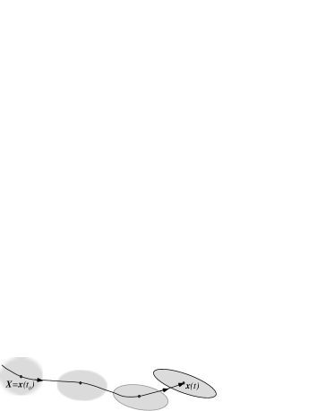
Figure 1: Sketch of how an initially uncertain (and thus modeled as isotropic) material element is mapped onto the present position ${\bf x}$ at time $t$, reflecting recent deformations.

To determine $P_{kk}$, we follow Ref. ChePum99 and use the Poisson equation $\nabla^{2}p=-A_{nm}A_{mn}=C^{-1}_{qq}P_{kk}/3$, from which $P_{kk}$ can be solved, leading to ChePum99

$$\frac{\partial^{2}p}{\partial x_{i}\partial x_{j}}=-\frac{C_{ij}^{-1}}{C_{qq}^{-1}}A_{nm}A_{mn}\mbox{ .}$$ (3)

A similar approach can be applied JeoGir to the viscous term, expressing the Laplacian of $A_{ij}$ in the Lagrangian frame, as in Eq. (2). The resulting Lagrangian Hessian of $A_{ij}$ is modeled by a classical linear damping term, namely $\nu{\partial^{2}A_{ij}}/{\partial X_{p}\partial X_{q}}\approx-\delta_{pq}A_{ij}/(3T)$. The relaxation time-scale $T$ is chosen to be on the order of the integral time-scale. This can be justified by recognizing that the distance travelled by a viscous eddy during a viscous turn-over or decorrelation time, advected by the rms turbulence velocity $u^{\prime}$, scales like the Taylor microscale, $\lambda$. Assuming therefore that $\lambda$ is the appropriate Lagrangian decorrelation length-scale of $A_{ij}$, it follows that $\nu/(\partial X)^{2}\sim\nu/\lambda^{2}\sim 1/T$. Finally, the model reads

$$\nu\frac{\partial^{2}A_{ij}}{\partial x_{m}\partial x_{m}}=-\frac{1}{T}\frac{C_{mm}^{-1}}{3}A_{ij}\mbox{ ,}$$ (4)

and is reminiscent of mapping closures Kra90 .

Replacing the pressure Hessian and the viscous term in Eq. (1) by the modeled terms Eqs. (3) and (4), one can show numerically that the finite-time divergence induced by the quadratic term is regularized, and each component of $A_{ij}$ tends to zero at long times. Next, to generate stationary statistics a stochastic forcing term can be added. The resulting system, however, is not stationary since it depends upon the evolving tensors D and C whose time evolutions reflect the non-stationary nature of turbulent dispersion. For example, on average the largest (resp. smallest) eigenvalue of C undergoes exponential growth (resp. decrease) in time, whereas the intermediate one remains approximatively constant MonYag ; GirPopJFM ; TsinoLag . We remark that in the tetrad model ChePum99 this feature is exploited to keep track of changing length scale. Our aim here is to develop a statistically stationary description of the velocity gradient at a fixed scale (e.g. viscous scale).

The crucial step of the proposed model is to replace the actual slow decorrelation along the Lagrangian trajectory and the total deformation history $[t_{0},t]$ with a perfect correlation of $A_{ij}$ during a time scale $\tau$ (which is thought to be of the order of the Kolmogorov time-scale $\sqrt{\nu/\epsilon}$, where $\epsilon$ is the dissipation rate). Correlations for time-delays longer than $\tau$ are neglected. It follows, using the time-ordered exponential property, that $\textbf{D}(t)=\textbf{D}(t-\tau)\textbf{D}_{\tau}(t)$, where $\textbf{D}_{\tau}(t)\approx e^{\tau\textbf{A}(t)}$. Furthermore, we neglect the prior deformation history. Accordingly, we may define a “stationary Cauchy-Green tensor”

$$\textbf{C}_{\tau}(t)=\textbf{D}_{\tau}(t)\textbf{D}_{\tau}^{T}(t)=e^{\tau\textbf{A}}e^{\tau\textbf{A}^{T}}\mbox{ .}$$ (5)

When $\tau$ decreases (i.e. the Reynolds number $\mathcal{R}_{e}$ increases), at fixed ${\bf A}$ the restitution strength of the pressure Hessian model decreases ($\tau=0$ corresponds to an isotropic pressure Hessian as in the singular RE system). Without loss of generality, henceforth all variables will be scaled with the time-scale $T$, i.e. $t/T\to t$ and $A_{ij}T\to A_{ij}$. Combining Eqs. (1), (3), (4), (5) and a forcing term, and defining the parameter $\Gamma\equiv\tau/T$ ($\sim\mathcal{R}_{e}^{-1/2}$), the following stochastic differential equation is finally obtained:

$$d\textbf{A}=\left(-\textbf{A}^{2}+\frac{\mbox{Tr}(\textbf{A}^{2})}{\mbox{Tr}(\textbf{C}_{\Gamma}^{-1})}\textbf{C}_{\Gamma}^{-1}-\frac{\mbox{Tr}(\textbf{C}_{\Gamma}^{-1})}{3}\textbf{A}\right)dt+d\textbf{W}\mbox{ .}$$ (6)

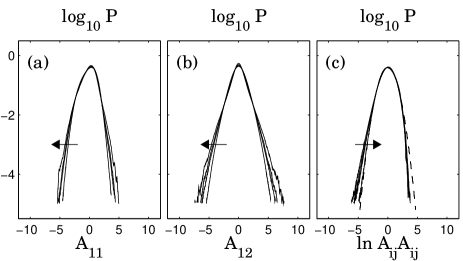
Figure 2: (a) and (b): PDFs of longitudinal and transverse components of the velocity gradient tensor A (normalized by its root-mean-square), obtained from time-integration of Eq. (6) for $\Gamma=0.2,0.1,0.08$ and 0.06. (c) PDF of $\ln A_{ij}A_{ij}$, for the same values of $\Gamma$. A Gaussian PDF of unit variance (dashed line) is also shown. Arrows direction indicates decreasing $\Gamma$ (increasing $\mathcal{R}_{e}$).

The tensorial noise $d\textbf{W}$ represents physical effects that have been neglected, such as action of larger-scale, and neighboring, eddies. For simplicity, we assume $d\textbf{W}$ is Gaussian and white in time. In the assumed units of time, we choose $d\textbf{W}=\textbf{G}\sqrt{2dt}$, where G is a tensorial Gaussian, delta-correlated noise. Its covariance matrix should be consistent with an isotropic, homogeneous, and traceless tensorial field, namely $\langle G_{ij}G_{kl}\rangle=2\delta_{ik}\delta_{jl}-\frac{1}{2}\delta_{ij}\delta_{kl}-\frac{1}{2}\delta_{il}\delta_{jk}$ PopBook . When $dW_{ij}=0$, numerical tests show that the finite-time divergence is regularized for any initial condition.

The stochastic differential equation (6) is solved numerically using four different values for $\Gamma$: 0.2, 0.1, 0.08 and 0.06. A second-order weak predicator-corrector scheme KloPla92 is used, with time steps $dt=10^{-2}$ ($dt=10^{-3}$ is used for $\Gamma=0.06$). Integration times of order $10^{5}~{}T$’s are used. Time-series of each component of A indicate stationary behavior. In Figs. 2(a-b) we show the PDFs of longitudinal ($A_{11}$) and transverse ($A_{12}$) components for various $\Gamma$ values (here and below, all statistics are improved by averaging over all available longitudinal and transverse directions, respectively). When $\Gamma$ decreases, velocity gradient PDFs develop slightly longer tails. Also, the longitudinal components are negatively skewed.

It has been observed in numerical simulations PopChe90 that the pseudo-dissipation $A_{ij}A_{ij}$ is close to lognormal for any Reynolds number (as obtained in the stationary diffusion process GirPop90_1 by specific construction of the nonlinear term), and one wonders whether lognormality arises in the present model. Fig. 2(c) presents the PDF of the logarithm of the pseudo-dissipation for various values of the parameter $\Gamma$. The PDF of $\ln A_{ij}A_{ij}$ from the model is close (but not exactly equal) to Gaussian. Note that the finiteness of dissipation implies that $\langle A_{11}^{2}\rangle/T^{2}=\epsilon/(15\nu)$. It follows that $\tau/\sqrt{\nu/\epsilon}$ is fixed through $\tau^{2}/(\nu/\epsilon)=15\langle A_{11}^{2}\rangle\Gamma^{2}$.

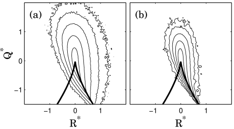
Figure 3: Contour plots of the logarithm of the joint probability of the two invariants of the velocity gradient tensor (see text) non-dimensionalized by the average strain, i.e. $Q^{*}=Q/\langle S_{ij}S_{ij}\rangle$ and $R^{*}=R/\langle S_{ij}S_{ij}\rangle^{3/2}$, for (a) $\Gamma=0.2$ and (b) $\Gamma=0.08$. Contours are logarithmically spaced, starting at 1 and separated by factors of 10. The thick line corresponds to zero discriminant (Vieillefosse line).

To further characterize the statistics of A, Fig. 3 presents the joint PDF of two important invariants of A, namely $Q=-\mbox{Tr}(\textbf{A}^{2})/2$ and $R=-\mbox{Tr}(\textbf{A}^{3})/3$, non-dimensionalized by $\langle S_{ij}S_{ij}\rangle$. The joint PDF in the RQ-plane shows the characteristic teardrope shape observed in various numerical and experimental studies GeoVortExpNum ; ChePum99 and is consistent with predominance of enstrophy-enstrophy production (top-left quadrant) and dissipation-dissipation production (bottom-right quadrant). For decreasing $\Gamma$, the joint PDF becomes more elongated along the right tail of the Vieillefosse line, consistent with data at increasing $\mathcal{R}_{e}$ GeoVortExpNum ; ChePum99 .

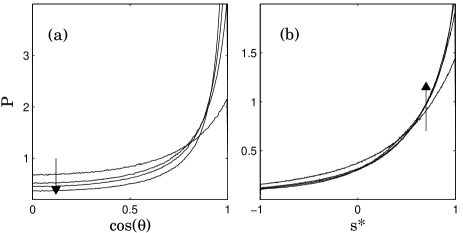
Figure 4: Alignment trends and preferred strain-rate state. In (a) is displayed the PDF of the cosine of the angle between vorticity and the intermediate eigenvector of the strain-rate tensor, showing preferential alignment. In (b), the PDF of the strain-rate state $s^{*}$ is presented.

Next, the statistics of alignment of the vorticity vector $\omega_{i}=\varepsilon_{ijk}A_{kj}$ with S, and the S-eigenvalues $\alpha$, $\beta$ and $\gamma$ are quantified. In Fig. 4(a) the PDF of $\cos(\theta)$, where $\theta$ is the angle between $\omega$ and the S-eigenvector corresponding to its intermediate eigenvalue, is shown. Clearly there is preferential alignment (as in numerical and experimental 3D flows GeoVortExpNum ). To quantify the preferred rate of strain state, we display in Fig. 4(b) the PDF of the parameter $s^{*}={-3\sqrt{6}\alpha\beta\gamma}/{(\alpha^{2}+\beta^{2}+\gamma^{2})^{3/2}}$. As in real flows GeoVortExpNum , the PDF of $s^{*}$ is shifted towards a peak at $s^{*}=1$ (axisymmetric expansion).

An important feature of small-scale turbulence is scaling of higher-order moments with $\mathcal{R}_{e}$ Nel90 , i.e. $\langle|A_{11}|^{p}\rangle\sim\mathcal{R}_{e}^{\mathcal{F}(p)}$. Regular K41 scaling corresponds to $\mathcal{F}(p)=p/2$ K41 while deviations indicate anomalous scaling. However, the simple assumption to take the forcing term W Gaussian and delta correlated in time is expected to be realistic at most for a limited range of Reynolds numbers. Therefore, we present results in terms of relative scaling which utilizes the above relation for $p=2$ to obtain $\mathcal{R}_{e}\sim\langle A_{11}^{2}\rangle$ (using $F(2)=1$ from the condition of finite dissipation), and thus $\langle|A_{11}|^{p}\rangle\sim\langle A_{11}^{2}\rangle^{\mathcal{F}(p)}$. Shown in Fig. 5 are $p$-order moments of $A_{11}$ and $A_{12}$, as functions of the second-order moments, and varying parameter $\Gamma$. Deviations from the dashed lines (K41 case with slope $p/2$) are consistent with anomalous scaling. Since PDFs of normalized $A_{11}$ and $A_{12}$ change with $\Gamma$ or $\mathcal{R}_{e}$, their statistics cannot follow K41 scaling. The solid lines in Fig. 5 use the multifractal formalism: $\mathcal{F}(p)=-\min_{h}\{[p(h-1)+1-\mathcal{D}(h)]/(h+1)\}$ and $\mathcal{D}(h)$ is the classical singularity spectrum Fri95 . The latter is used here with a parabolic approximation $\mathcal{D}(h)=1-{(h-c_{1})^{2}}/{(2c_{2})}$, with $c_{1}=1/3+3c_{2}/2$ Nel90 ; CheCas06 , and thus a single unknown parameter $c_{2}$ ($c_{2}=\mu/9$, where $\mu$ is the usual intermittency exponent). The numerical results can thus be used to determine $c_{2}$ from the model by fitting the slopes in Fig. 5. The solid lines are for a parameter $c_{2}=0.025$ (or $\mu=9c_{2}\sim 0.22$) for the longitudinal, and $c_{2}=0.040$ for the transverse cases. These values are in excellent agreement with values found from experiments and DNS Fri95 ; CheCas06 . The longitudinal derivative skewness factor $\mathcal{S}$ shows characteristic values near $-0.5$.

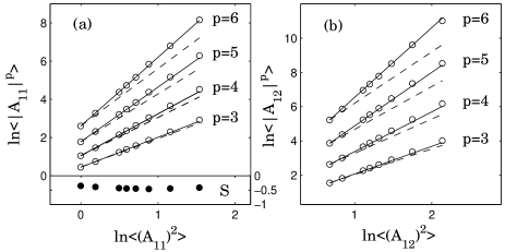
Figure 5: Relative scaling of velocity gradient moments ($\circ$) in the (a) longitudinal direction and (b) transverse direction for various orders $p$. Different points are for various $\Gamma$ (from left to right $\Gamma=$ 0.2, 0.15, 0.1, 0.09, 0.08, 0.07, 0.06, and 0.05). In (a) the skewness coefficient of longitudinal components $\mathcal{S}=\langle A^{3}_{11}\rangle/\langle A_{11}^{2}\rangle^{3/2}$ is also shown ($\bullet$ using the right scale). Solid lines denote predictions from multifractal scaling, dashed lines are Kolmogorov (1941) non-anomalous scaling.

In conclusion, building on several prior works Can91 ; GirPop90_1 ; ChePum99 ; JeoGir , a new model has been proposed for the anisotropic part of the pressure Hessian and the viscous diffusion term entering in the Lagrangian evolution equation for the velocity gradient tensor A. The system predicts a variety of local, statistical, geometric and anomalous scaling properties of 3-D turbulence. Results are obtained within a limited range of the parameter $\Gamma$, or Reynolds number $\mathcal{R}_{e}$. When tests are done with $\Gamma$ below 0.05, the PDFs of velocity increments, of $R$ and $Q$, and alignment trends become less realistic. This is due possibly to the limitations imposed by the assumption of Gaussian forcing. More work is needed to extend the approach to arbitrarily high Reynolds numbers, possibly by adding additional degrees of freedom to the model or by modifying the type of forcing. Moreover, establishing connections with the statistics of Lagrangian structure functions (velocity increments in time instead of the spatial variations described by $A_{ij}$) requires additional models to describe jointly the Lagrangian evolution of velocity and velocity gradients.

We gratefully acknowledge the Keck Foundation (LC) and the National Science Foundation (CM) for financial support. We thank L. Biferale for his very insightful comments, and Y. Li, Z. Xiao, B. Castaing, G. Eyink, E. Vishniac, S. Chen and A. Szalay for fruitful discussions.

References

- (1) A.N. Kolmogorov, Dokl. Akad. Nauk SSSR 30, 301 (1941); also Proc. R. Soc. A 434, 9 (1991).
- (2) U. Frisch, Turbulence (CUP, Cambridge, 1995).
- (3) L. Chevillard et al., Physica D 218, 77 (2006).
- (4) Y. Li and C. Meneveau, Phys. Rev. Lett. 95, 164502 (2005), J. Fluid Mech. 558, 133 (2006).
- (5) B.W. Zeff et al., Nature 421, 146 (2003).
- (6) B.J. Cantwell, Phys. Fluids A 5, 2008 (1993). W.T. Ashurst et al., Phys. Fluids 30, 2343 (1987). T.S. Lund and M.M. Rogers, Phys. Fluids 6, 1838 (1994). A. Tsinober, E. Kit, T. Dracos, J. Fluid Mech. 242, 169 (1992). A. Tsinober, An informal introduction to turbulence (Kluwer Academic Publishers, Dordrecht, 2001). F. van der Bos et al., Phys. Fluids 14, 2457 (2002).
- (7) P. Vieillefosse, Physica A 125, 150 (1984).
- (8) B.J. Cantwell, Phys. Fluids A 4, 782 (1992).
- (9) S.S. Girimaji and S.B. Pope, Phys. Fluids A 2, 242 (1990).
- (10) J. Martin et al., Phys. Fluids 10, 2336 (1998).
- (11) M. Chertkov, A. Pumir, and B.I. Shraiman, Phys. Fluids 11, 2394 (1999). A. Naso and A. Pumir, Phys. Rev. E 72, 056318 (2005).
- (12) E. Jeong and S.S. Girimaji, Theor. Comput. Fluid Dyn. 16, 421 (2003).
- (13) P. Constantin, Commun. Math. Phys. 216, 663 (2001).
- (14) A.S. Monin and A.M. Yaglom, Statitistical Fluid Mechanics (MIT Press, Cambridge, MA, 1975).
- (15) S.S. Girimaji and S.B. Pope, J. Fluid Mech. 220, 427 (1990).
- (16) B. Luthi, A. Tsinober and W. Kinzelbach, J. Fluid Mech. 528, 87 (2005).
- (17) G. Falkovich, K. Gawedzki and M. Vergassola, Rev. Mod. Phys. 73, 913 (2001).
- (18) R.H. Kraichnan, Phys. Rev. Lett. 65, 575 (1990).
- (19) S.B. Pope and Y.L. Chen, Phys. Fluids A 2, 1437 (1990).
- (20) P.E. Kloeden, E. Platen, Numerical solution of Stochastic Differential Equations (Springer, Berlin, 1999).
- (21) S.B. Pope, Turbulent flows (CUP, Cambridge, 2000).
- (22) M. Nelkin, Phys. Rev. A 42, 7226 (1990).