Topological solitons in highly anisotropic two dimensional ferromagnets

Abstract

We study the solitons, stabilized by spin precession in a classical two–dimensional lattice model of Heisenberg ferromagnets with non-small easy–axis anisotropy. The properties of such solitons are treated both analytically using the continuous model including higher then second powers of magnetization gradients, and numerically for a discrete set of the spins on a square lattice. The dependence of the soliton energy $E$ on the number of spin deviations (bound magnons) $N$ is calculated. We have shown that the topological solitons are stable if the number $N$ exceeds some critical value $N_{\rm{cr}}$. For $N<N_{\rm{cr}}$ and the intermediate values of anisotropy constant $K_{\mathrm{eff}}<0.35J$ ($J$ is an exchange constant), the soliton properties are similar to those for continuous model; for example, soliton energy is increasing and the precession frequency $\omega(N)$ is decreasing monotonously with $N$ growth. For high enough anisotropy $K_{\mathrm{eff}}>0.6J$ we found some fundamentally new soliton features absent for continuous models incorporating even the higher powers of magnetization gradients. For high anisotropy, the dependence of soliton energy $E(N)$ on the number of bound magnons become non-monotonic, with the minima at some ”magic” numbers of bound magnons. Soliton frequency $\omega(N)$ have quite irregular behavior with step-like jumps and negative values of $\omega$ for some regions of $N$. Near these regions, stable static soliton states, stabilized by the lattice effects, exist.

I Introduction

An analysis of two-dimensional (2D) magnetic solitons has been an active area of research for more then 30 years, see Refs. Kosevich90, ; Bar'yakhtar93, ; Bar'yakhtar94, ; ZaspelDrumh, ; Mertens00, for review. Such solitons are known to play an important role in the physics of 2D magnetic systems. In the easy–plane magnets with continuously degenerate ground state there appear magnetic vortices, responsible for the Berezinskii–Kosterlitz–Thouless (BKT) phase transition Berezinsky72 ; Kosterlitz73 . The presence of vortices leads to the emergence of a central peak in dynamical response functions of a magnet,Mertens89 which can be observed experimentally Wiesler89 . There are no vortices in the easy–axis magnets with discretely degenerate ground state, but various types of localized topological solitons appear there. Belavin and Polyakov were the first to construct the exact analytical solutions for 2D topological solitons in a continuous model of the isotropic magnetBelavin75 . The energy of such Belavin - Polyakov (BP) solitons $E_{BP}$ in a magnet with exchange constant $J$ is finite and described by the universal relation

$$E_{\rm{BP}}=4\pi JS^{2},$$ (1)

$S$ is the atomic spin. The structure of such solitons is described by a topologically nontrivial distribution of the magnetization field $\vec{m}(x,y)$,Kosevich90 which is determined by the $\pi_{2}$ topological invariant, see below Eq. (12) and Refs.Topology, for more details. Belavin and Polyakov have also proved that such solitons are responsible for the destruction of the long–range magnetic order in purely continuous isotropic models at any finite temperature. Belavin75 The studies of topological solitons has become interesting now due to their possible application in high–energy physics,Walliser00 and the quantum Hall effect Prange90 . Also, such soliton solutions after the change $y\to c\tau$ ($\tau$ is an imaginary time, $c$ is the speed of magnons) determine so-called instantons, describing non-small quantum fluctuations in 1D isotropic antiferromagnetsAffleck .

Note that the properties of the solitons in this isotropic model is rather academic problem since all real magnets have a discrete lattice structure and non-zero anisotropy. The role of uniaxial anisotropy has been investigated in a number of articles, see. Refs. Kosevich90, ; Bar'yakhtar93, for review. Topological solitons of the same $\pi_{2}$ topological structure are also inherent for standard continuum (with accounting of terms quadratic on the magnetization field gradients, like the term $W_{2}$ in the first line of Eq. (9) below) models of anisotropic magnets. The basic problem of soliton physics in 2D magnets is related to soliton stability. According to the famous Hobard–Derrick theorem,Hobard63 ; Derrick64 the stable static non–one–dimensional soliton with finite energy and finite radius does not exist in the standard nonlinear field models; the soliton is unstable against collapse. This is, in particular, true for the uniaxial 2D ferromagnet with the anisotropy energy density ${\cal W}_{a}\propto m_{x}^{2}+m_{y}^{2}$.

The possibility to construct non–one–dimensional solitons stable against collapse is due to the presence of additional integrals of motion. For example, such solitons can be realized in the uniaxial ferromagnet due to the conservation of $z$–projection of the total spin Kosevich90 ; Bar'yakhtar93 . This leads to the appearance of so–called precessional solitons characterizing by time-independent projection of magnetization onto the easy axis ($z$-axis hereafter), with the precession of the magnetization vector $\vec{m}$ at constant frequency around the $z$ axis. The analogies of such precessional solitons are known to occur in different models of field theory and condensed matter physics, see Ref. Makhankov78, for review. Here the stability of 2D solitons is not related directly to their topological properties; the non–topological dynamical solitons may also exist in magnets. Such solitons are characterized by the spatially localized function $\vec{m}(x,y)$, which does not have nontrivial topological properties. All stable precessional solitons, topological and non-topological, realize the minimum of energy for a given number of spin $S_{z}$ deviations. In the semiclassical approximation, this value can take integer values $N$ only, and can be interpreted as a number of magnons excited in the magnet. Thus, we naturally arrive at the concept of a soliton as a bound state of a large number of magnons Kosevich90 .

Two - parameter (parameters are precession frequency and velocity of translational motion of a soliton) small-amplitude non-topological magnetic solitons moving with arbitrary velocity in a two-dimensional easy - axis ferromagnet have been constructed in Ref.IvZaspYastr, . Their minimal energy $E_{\rm{NT}}=11.7JS^{2}$ depends only on combination $JS^{2}$ similar to Eq. (1), which is a bit smaller then the energy of above discussed Belavin-Polyakov soliton, $E_{\rm{NT}}=0.93E_{\rm{BP}}$. For such solitons, the relation between their energy (for given $N$) and momentum can be thought of as their dispersion law. Near the minimal energy $E_{\rm{NT}}$, this dispersion law has a form $E(P,N)\simeq\varepsilon(P)\cdot N$, where $\varepsilon(P)$ is a dispersion law for linear magnons. For $P=0$, this gives the critical number of bound magnons $N_{c}=E_{\rm{NT}}/\varepsilon(0)$. Thus, these solitons are nothing but weakly coupled magnon clouds, see Fig. 2 below. The expression for the soliton dispersion law is used to calculate the soliton density and the soliton contributions to thermodynamic quantities (response functions) like specific heat. The signature of soliton contribution to the response functions of a magnet is an Arrhenius temperature dependence like $\exp(-E_{0}/T)$ with the characteristic value $E_{0}$ as a soliton energy. Such behavior with $E_{\rm{NT}}$ $\leq E_{0}\leq$ $E_{\rm{BP}}$ has been observed experimentally in Refs. Waldner+, ; Zaspel+, , see Ref. ZaspelDrumh, for review. Comparison of contributions from solitons and free magnons shows that there is a wide temperature range where the solitons give more important contribution to thermodynamic functions such as heat capacity or density of spin deviations.

We note here, that the structure of these non-topological solitons for $E\geq E_{\rm{NT}}$ is essentially different from that of topological solitons in uniaxial magnets. Namely, as $E\to E_{\rm{BP}}$, the radius of topological soliton in continuous model of anisotropic magnets diminishes, making them ”more localized”, contrary to non–topological solitons, which become delocalized as $E\to E_{\rm{NT}}$. Hence, although the energy of topological solitons is a little larger then that of non–topological solitons (0.89 and 1 in the units of $E_{\rm{BP}}$, see above), it is possible that only BP-type topological solitons would contribute to response functions measured by neutron scattering in the region of non-small momentum transfer. On the other hand, recent Monte-Carlo simulations for 2D discrete models of easy-axis magnets did not show any signatures of small-radius topological solitons Wysin+ .

For real magnets, which are discrete spin systems on a lattice, there is an additional problem of application of the topological arguments, which, strictly speaking, can be applied only to continuous functions ${\vec{m}}({\vec{r}},t)$. It is widely accepted that the continuous description is valid for discrete systems if the characteristic scale $l_{0}$ of magnetization ${\vec{m}}({\vec{r}},t)$ variation, $|\nabla{\vec{m}}|\sim{\vec{m}}/l_{0}$, is much larger than lattice constant $a$. The analysis of the magnetic vortices have shown that $\pi_{1}-$ topological charge of a vortex is determined by the behavior at infinities only so that the topological structure of such a vortex survives even in ”very discrete” models with $l_{0}<a$. As for our case of $\pi_{2}$ topological charge, the situation is not so simple and obvious. From one side, the continuous approach describes quantitatively the magnetization distribution in the vortex core already at $l_{0}\approx 1.5a$Ivanov96 . On the other side, so-called cone state vortices, with different energies for two possible spin directions in the vortex core are much more sensitive to the anisotropy, in fact, to the parameter $a/l_{0}$. Even for $l_{0}>10a$ their $\pi_{2}-$ topological charge (polarization $p\equiv m_{z}(0)=\pm 1$), characterizing the core structure of vortices, for heavy vortices with higher energy can change so that they convert into more preferable light vortices with opposite polarization $p$,IvWysin02 that never happened for continuum model IvSheka . Thus, the role of the discreteness effects is quite ambiguous.

The above situation resembles the one-dimensional case - there are also kinks and breathers (non–topological solitons) with smaller energy. But it is well-known, that in the 1D case for low anisotropy only kinks contribute to the response functions since small energy breathers transit continuously into weakly coupled magnon conglomerates. We note that for such systems in one space dimension, the difference between topological and non-topological solitons for high anisotropy is not that large. For instance, the spin complexes with several $N\sim 10$ magnons have been observed in a chain material CoCl${}_{2}\cdot$ 2H₂O with high Ising - type anisotropy ExperCsCl2 . These complexes can be interpreted as non-topological one-dimensional solitons.

The present work is devoted to the analysis of 2D solitons, both topological and non-topological, in the strongly anisotropic magnets accounting for discreteness effects. In other words, here we investigate the influence of finiteness of $a/l_{0}$ on the soliton structure. For intermediate values of anisotropy we found the presence of the critical number of bound magnons $N_{\mathrm{cr}}$: the topological soliton is stable at $N>N_{\mathrm{cr}}$ only. For very large anisotropy we found the specific effects of non-monotonic dependence of soliton properties on the number of bound magnons, caused by discreteness leading to the presence of ”magic” magnon numbers.

II The discrete model and its continuous description

We consider the model of a classical 2D ferromagnet with uniaxial anisotropy, described by the following Hamiltonian

$${\mathcal{H}}=-\sum_{{\vec{n}},{\vec{a}}}\!\left(J\vec{S}_{\vec{n}}\!\cdot\!\vec{S}_{{\vec{n}}+{\vec{a}}}+\kappa S^{z}_{\vec{n}}S^{z}_{{\vec{n}}+{\vec{a}}}\right)+$$

$$+K\sum_{\vec{n}}[(S^{x}_{\vec{n}})^{2}+(S^{y}_{\vec{n}})^{2}].$$ (2)

Here $\vec{S}\equiv\left(S^{x},S^{y},S^{z}\right)$ is a classical spin vector with fixed length $S$ on the site $\vec{n}$ of a 2D square lattice. The first summation runs over all nearest–neighbors ${\vec{a}}$, $J>0$ is the exchange integral, and the constant $\kappa$ describes the anisotropy of spin interaction. In subsequent discussion, we will refer to this type of anisotropy as exchange anisotropy (ExA). Additionally, we took into account single-ion anisotropy (SIA) with constant $K$. We consider the $z$–axis as the easy magnetization direction so that $K>0$ or $\kappa>0$.

In quantum case, the Hamiltonian (II) commutes with $z-$projection of total spin. It is more convenient to use semiclassical terminology, and to present it as a number of bound magnons in a soliton $N$, defined by the equation

$$N=\sum_{\vec{n}}\left(S-S^{z}_{\vec{n}}\right).$$ (3)

The spin dynamics is described by Landau–Lifshitz equations

$$\frac{d\vec{S}_{\vec{n}}}{dt}=-\frac{1}{\hbar}\left[\vec{S}_{\vec{n}}\times\frac{\partial\mathcal{H}}{\partial\vec{S}_{\vec{n}}}\right].$$ (4)

In the case of weak anisotropy, $K,\ \kappa\ll J$, the characteristic size of excitations $l_{0}\gg a$, see Eq. (14) below, so that the magnetization varies slowly in a space. In this case we can introduce the smooth function $\vec{S}(x,y,t)$ instead of variable $\vec{S}_{n}(t)$ and use a continuous approximation for the Hamiltonian (II). It is based on the expansion of a classical magnetic energy $E$ in power series of magnetization ${\vec{S}}$ gradients,

$$E=W_{2}+W_{4}+...,$$ (5)

where $W_{2}$ contains zeroth and second order contributions to magnetic energy and $W_{4}$ contains the fourth powers. These are given by

$$W_{2} = \int d^{2}x\Biggl{\{}\frac{K_{\rm{eff}}}{a^{2}}(S^{2}-S_{z}^{2})+\frac{J}{2}\left(\nabla{\vec{S}}\right)^{2}+$$ (6a)

$$+ \frac{\kappa}{2}\left(\nabla S_{z}\right)^{2}\Biggl{\}},$$

$$W_{4} = -\frac{a^{4}}{24}\int d^{2}x\Biggl{\{}J\left[\left(\frac{\partial^{2}{\vec{S}}}{\partial x^{2}}\right)^{2}+\left(\frac{\partial^{2}{\vec{S}}}{\partial y^{2}}\right)^{2}\right]+$$ (6b)

$$+ \kappa\left[\left(\frac{\partial^{2}S_{z}}{\partial x^{2}}\right)^{2}+\left(\frac{\partial^{2}S_{z}}{\partial y^{2}}\right)^{2}\right]\Biggr{\}},$$

where $\nabla$ is a 2D gradient of the function ${\vec{S}}({\vec{r}},t)$. Here, we used integrations by parts with respect to the fact that our soliton texture is spatially localized. We omit unimportant constants and limit ourselves to the terms of fourth order only as they are playing a decisive role in stabilization of solitons, see for details Ivanov86 ; IvWysin02 . Also, we introduce the effective anisotropy constant

$$K_{\rm{eff}}=K+2\kappa.$$ (7)

We note here, that single-ion anisotropy enters only $W_{2}$, but not $W_{4}$ and higher terms, while exchange anisotropy enters every term of the above expansion over powers of magnetization gradients. Usually, this difference is not important for small anisotropy, $K,\ \kappa\ll J$, but, as we will see below, this fact gives qualitatively different behavior near the soliton stability threshold.

Introducing the angular variables for normalized magnetization

$$\vec{m}=\frac{\vec{S}}{S}=\left(\sin\theta\cos\phi;\sin\theta\sin\phi;\cos\theta\right),$$ (8)

we obtain the following form of the classical magnetic energy

$$E[\theta,\phi] = W_{2}+W_{4},\ W_{2}=JS^{2}\int d^{2}x\left\{\frac{K_{\rm{eff}}}{a^{2}}\sin^{2}\theta+\frac{1}{2}\left[\left(\nabla\theta\right)^{2}\left(1+\kappa\sin^{2}\theta\right)+\left(\nabla\varphi\right)^{2}\sin^{2}\theta\right]\right\},$$

$$W_{4} = -\frac{1}{24}Ja^{2}S^{2}\int d^{2}x\Biggl{\{}\left(\nabla^{2}\theta\right)^{2}\left[1+\kappa\sin^{2}\theta\right]+\left(\nabla\theta\right)^{4}\left[1+\kappa\cos^{2}\theta\right]+$$ (9)

$$+\sin^{2}\theta\left(\nabla\varphi\right)^{2}\left[\left(\nabla\varphi\right)^{2}+2\left(\nabla\theta\right)^{2}\right]+2\sin\theta\cos\theta(\nabla^{2}\theta)\left[\kappa\left(\nabla\theta\right)^{2}-\left(\nabla\varphi\right)^{2}\right]\Biggr{\}}.$$

In this long expression we omitted the terms with scalar product of gradients like $(\nabla\theta,\,\nabla\phi)$, because they do not contribute to the trial function we will use for analysis, see below.

In terms of fields $\theta$ and $\phi$, the continuous analog of Landau–Lifshitz equations (4) read

$$\sin\theta\frac{\partial\phi}{\partial t}=\frac{a^{2}}{\hbar S}\frac{\delta E}{\delta\theta},\quad\sin\theta\frac{\partial\theta}{\partial t}=-\frac{a^{2}}{\hbar S}\frac{\delta E}{\delta\phi}.$$ (10)

These equations can be derived from the Lagrangian

$$\mathcal{L}[\theta,\phi]=-\frac{\hbar S}{a^{2}}\int d^{2}x(1-\cos\theta)\frac{\partial\phi}{\partial t}-E[\theta,\phi].$$ (11)

The simplest nonlinear excitation of the model (11) with $E\equiv W_{2}$ is the 2D localized soliton, characterized by the homogeneous distribution of magnetization far from its core. Topological properties of the soliton are determined by the mapping of physical $XY$–plane to the $\mathbb{S}^{2}$–sphere given by the equation $\mathbf{m}^{2}=1$ of the order parameter space. This mapping is described by the homotopy group $\pi_{2}(\mathbb{S}^{2})=\mathbb{Z}$, see, Topology which is characterized by the topological invariant (Pontryagin index)

$$Q=\frac{1}{8\pi}\int\limits_{S^{2}}d^{2}x\;\varepsilon_{\alpha\beta}\left[\vec{m}\cdot\bigl{(}\nabla_{\alpha}\vec{m}\times\nabla_{\beta}\vec{m}\bigr{)}\right]=\\ =\frac{1}{4\pi}\int\limits_{S^{2}}\sin\theta\;d\theta\;d\phi,$$ (12)

taking integer values, $Q\in\mathbb{Z}$. Here $\varepsilon_{\alpha\beta}$ is Levi-Civita tensor.

To visualize the structure of a topological soliton, we consider the case of a purely isotropic magnet with $K_{\rm{eff}}=0$ and $W_{4}=0$. For this isotropic continuous model the soliton solution is aforementioned BP soliton of the form Belavin75

$$\tan\frac{\theta}{2}=\left(\frac{R}{r}\right)^{|Q|},\quad\phi=\varphi_{0}+Q\chi,$$ (13)

where $r$ and $\chi$ are polar coordinates in the $XY$–plane, $\varphi_{0}$ is an arbitrary constant. The energy (1) of this soliton does not depend of its radius $R$, which is arbitrary parameter for the isotropic magnet, see Ref. Belavin75, . However, even small anisotropy breaks the scale invariance of the above model since now the scale

$$l_{0}^{2}=\frac{a^{2}J}{2K_{\rm{eff}}}$$ (14)

enters the problem.

In the latter case, the soliton energy with respect to $W_{2}$ term only has the form $E=E_{\rm{BP}}+{\rm{const}}\cdot(R/l_{0})^{2}$ and hence has a minimum at $R=0$ only, which signifies the instability of the static soliton against collapse in this model. Obviously, the scale invariance is also broken in the initial discrete model. The ”trace of discreteness” in our continuous model (11) is the presence of a contribution $W_{4}$. This term gives the contribution to the soliton energy proportional to $JS^{2}a^{2}/R^{2}$. For some rather exotic models containing higher powers of a magnetization field gradients like $\left(\vec{\nabla}\vec{m}\right)^{4}$ (with positive sign), Skirm61 ; Hobard65 ; Enz77a ; Enz78 such term might be able to stabilize even static soliton against collapse, see Ivanov86 for details. However, for Heisenberg magnets this kind of stabilization is very problematic. For example, discrete magnetic models with the Heisenberg interaction of nearest neighbors only (i.e. those without biquadratic exchange and/or next–nearest–neighbors interaction) have negative $W_{4}<0$, and the higher powers of magnetization gradients do not stabilize a static soliton in this case. Moreover, as we will show below, the presence of discreteness ruins the stability of the precessional soliton with $N<N_{\mathrm{cr}}$ even in the case, when it is stable in the simplest model with $W=W_{2}$ only.

We now discuss the stability of precessional solitons. For a purely uniaxial ferromagnet the energy functional $E[\theta,\phi]$ does not depend explicitly on the variable $\phi$ so that there exists an additional integral of motion,Kosevich90 which is the continuous analog of Eq.(3)

$$N=\frac{S}{a^{2}}\int d^{2}x\left(1-\cos\theta\right).$$ (15)

The conservation law (15) can provide a conditional (for constant $N$) minimum of the energy functional $E$, stabilizing the possible soliton solution. Namely, we may look for an extremum of the expression

$$L=E-\hbar\omega N,$$ (16)

where $\omega$ is an internal soliton precession frequency, that can be regarded as a Lagrange multiplier. Note that this functional is nothing but the Lagrangian (11) calculated with respect to specific time dependence

$$\phi=\omega t+Q\chi+\varphi_{0},$$

which holds instead of (13) in this case. This condition leads to the relation,Kosevich90

$$\hbar\omega=\frac{dE}{dN},$$ (17)

which makes clear the microscopic origin of the precessional frequency $\omega$. Namely, an addition of one extra spin deviation (bound magnon) to the soliton changes its energy by $\hbar\omega$. Thus, the dependence $\omega(N)$ is extremely important for the problem of a soliton stability. For the general continuous model of a ferromagnet, even containing the terms like $W_{4}$, the sufficient and necessary condition of soliton stability reads $d\omega/dN<0$,Zhmudsky97 but for the discrete model the validity of this condition is not clear yet. The point is that the known analytical methods of a soliton stability analysis rely essentially on the presence of a zeroth (translational) mode, which is obviously present for any continuous model, but is absent for discrete models, where lattice pinning effects are present. To solve the problem of soliton stability we will investigate explicitly the character of conditional extremum of the energy with $N$ fixed.

III The methods of a soliton structure investigations

To get the explicit soliton solution and investigate its stability we have to solve the Landau-Lifshitz equations (10) with respect to the energy (9). For the simplest model accounting for $W_{2}$ only, an exact ansatz

$$\theta=\theta(r),\ \phi=Q\chi+\omega t\;,$$ (18)

can be used, leading to the ordinary differential equation for the function $\theta(r)$. This equation can be easily solved numerically by shooting procedure, using the value of $d\theta/dr$ at $r=0$ as a shooting parameter, see Ref. Kosevich90, . The shape of the soliton essentially depends on the number $N$ of bound magnons. In the case of the soliton with large $N\gg N_{2}\equiv 2\pi S(l_{0}/a)^{2}$), the approximate ”domain wall” solution works pretty well. This solution has the shape of a circular domain wall of radius $R$

$$\cos\theta_{0}(r)=\tanh\frac{r-R}{l_{0}}.$$ (19)

Using this simple structure one can obtain the number of bound magnons, which is proportional to the size of the soliton, $N\approx 2\pi S(R/a)^{2}$ and energy, $E=4\pi S^{2}\sqrt{2JK_{\rm{eff}}}R/a$. Note that such a solution is the same for topological and non-topological solitons except for the behavior near the soliton core. This means, that the characteristics of such solitons are pretty similar. In the case of the small radius soliton ($R\ll l_{0}$), the following asymptotically exact solution works well Voronov83

$$\tan\frac{\theta_{0}(r)}{2}=\frac{R}{r_{0}}\ K_{1}\left(\frac{r}{r_{0}}\right),\qquad r_{0}=\frac{l_{0}}{\sqrt{1-\omega/\omega_{0}}},$$ (20)

where $K_{1}(x)$ is the McDonald function, and $\omega_{0}$ is a gap frequency for linear magnons. It provides correct behavior at $r<R\ll l_{0}$, where it converts to the Belavin–Polyakov solution (13). For large distances ($r\gg R$), this expression gives an exponential decay (instead of power decay for a Belavin-Polyakov soliton) with characteristic scale $r_{0}$. For solution (20) $\omega\to\omega_{0}$ as $N\to 0$ so that small radius solitons in anisotropic magnets have two different scales, the core size $R\ll l_{0}$ and the scale of the exponential “tail” $r_{0}=l_{0}/\sqrt{1-\omega/\omega_{0}}\gg l_{0}$ Voronov83 ; Ivanov86 .

For even minimal accounting for the discreteness on the basis of a generalized model with fourth spatial derivatives, the problem becomes much more complicated. The complexity of the problem is not only due to the fact that for the energy (9) it is necessary to solve the fourth order differential equation, and use a much more complicated three-parameter shooting method. But the basic complication here is the fact that in general fourth-derivative terms contain anisotropic contributions like $(\partial^{2}\theta/\partial x^{2})^{2}+(\partial^{2}\theta/\partial y^{2})^{2}$, which cannot be reduced to the powers of radially-symmetric Laplace operator (these terms are omitted in Eq. (9) for simplicity). In this case, the radially-symmetric ansatz with $\theta=\theta(r),\,\phi=\phi(\chi)$ is not valid, and we have to solve a set of partial nonlinear differential equation for the functions $\theta=\theta(r,\chi),\ \phi=\phi(r,\chi)$. To the best of our knowledge, an exact method for construction of soliton (separatrix) solutions for such type of equations do not exist so that some other approximate methods should be used for this problem.

III.1 Variational approach for general continuum model

One of the approaches, which we use for the approximate analysis of the solitons in the model (9), is the direct variational method. For the minimization of the energy $E=W_{2}+W_{4}$ we use a trial function,

$$\tan\frac{\theta}{2}=\Lambda RK_{1}\left(\Lambda r\right).$$ (21)

Here, we consider the case $Q=1$, and the case of higher topological invariants is qualitatively similar. Note, that trial function (21) is based on the asymptotically exact soliton solution (20). The trial function (21) gives correct asymptotics both for $x\to 0$ (corresponding to BP soliton) and for $x\to\infty$ (exponential decay with characteristic scale $1/\Lambda$), see above. Our analysis shows that the same results can be obtained using a simplified trial function, which also captures the asymptotic behavior of the soliton. This function has the form

$$\tan\frac{\theta}{2}=\frac{R}{r}\exp(-\Lambda r).$$ (22)

In the spirit of the minimization method above discussed we consider the parameter $\Lambda$ as variational, keeping the parameter $R$ constant as it is related to $N$, $N\propto R^{2}$, see, e.g.. Kosevich90 In other words, we minimize the energy (9) with the trial function (21) or (22) over $\Lambda$ for constant $R$. This approach has the advantage that simultaneously with equation solving, it permits investigation of the stability of obtained solution on the base of simple and obvious criterion. Namely, a soliton is stable if it corresponds to the conditional minimum of the energy at fixed $N$, and it is unstable otherwise.

III.2 Numerical analysis of the lattice model

Since the continuous description fails for the case of a high anisotropy, one needs to elaborate the discrete energy (II) on a lattice. As we are not able to solve the problem analytically, we discuss the numerical approach to study the soliton-like spin configurations on a discrete square lattice. Obviously, the direct molecular dynamics simulations on a lattice is a powerful tool for the soliton investigation for any values of anisotropy. Direct spin dynamics simulations of 2D solitons have been recently performed in Refs. Kamppeter01, ; Sheka+ivanov+EuJP06, . After the relaxation scheme, where an initial trial solution was fitted to the lattice, the spin–dynamical simulations of the discrete Landau-Lifshitz equations were performed. This approach, however, is quite computer intensive, requiring powerful computers. To minimize the calculation time, the parallel algorithms have been used Sheka+ivanov+EuJP06 .

For this reason, we obtained desired spin configuration by direct minimization of the energy $E$, keeping $N$ constant. For our modeling we choose the square lattices with ”circular” boundary conditions. We fix the values of spins on the boundary to the ground state ($\theta=0$), those values have been kept intact during minimization. The method of minimization is the simplex type method with non-linear constraints. This method is based on the steepest descent routine applied to the functions of a large number of variables. The above method is able to find the conditional minimum of a given function with several (usually small number) constraints, consisting of relations between variables. In our problem, such variables are the directions of each spin, parameterized by the angular variables $\theta_{n}$ and $\varphi_{n}$, and the conditional minimum of the energy, $E$ has been obtained for a fixed value of $z-$ projection of the total spin. As this additional constraint slows down the calculations substantially, we use other method, valid for initial configurations where $N$ differs from the necessary quantity by one spin. The idea of the method is as follows: the angle $\theta$ of an arbitrarily chosen ”damper” spin was excluded from the minimization procedure, and its value has been kept constant, to achieve the necessary $N$ value throughout whole minimization with respect to all other variables.

The method in fact is dealing formally with a static problem, but it gives the possibility to find the precessional frequency directly. To find $\omega$, we used the discrete Landau-Lifshitz equation (4) rewritten for the angular variable $\phi_{n}$, in the way used in equation (10). Using relation $\partial\phi_{n}/\partial t=\omega$, we obtain

$$\omega=\frac{1}{\sin\theta_{n}}\cdot\frac{1}{\hbar S}\frac{\partial\mathcal{H}}{\partial\theta_{n}}\ ,$$ (23)

which does not depend on index $n$ throughout all the system. Here $\mathcal{H}$ is the discrete Hamiltonian (II).

To find the above local minimum, we start from the BP initial configuration. The size of lattice clusters varied from $20\times 20$ (for large anisotropies, where discreteness of a lattice is revealed most vividly) to $32\times 32$ for small anisotropy when system is well described by a continuous model. The criterion of the presence of a truly local soliton configuration was its independence of the system size. Another important criterion was the constancy of the frequency $\omega$, calculated from the equation (23) throughout the soliton configuration. Sometimes we found the minimum over the variables $\theta_{n}$ only, considering $\phi_{n}$ to obey Eq. (18) and choosing the reference frame origin in the symmetric points between the lattice sites. Our analysis has shown that for moderate anisotropies $K_{\rm{eff}}\lesssim 0.5J$ the above partial minimization gives the same energy and frequency as well as the instability point position, as complete minimization over $\theta_{n}$ and $\phi_{n}$. The use of partial minimization over $\theta_{n}$ permits not only to accelerate the numerical calculations, but turns out to be useful for construction of ”quasitopological”  textures for extremely high anisotropies, see below, Section V.

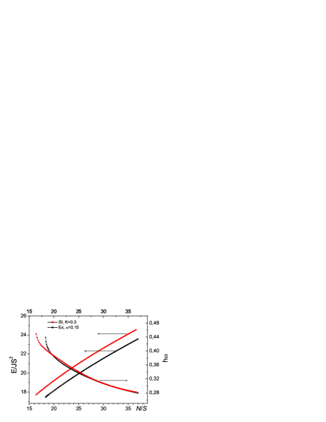
Figure 1: Dependence $E(N)$ and $\omega(N)$ for a soliton with $K_{\rm{eff}}=0.3$, obtained from numerical simulations.

In Fig.1, the dependence of a soliton energy and precession frequency, is shown as a function of the bound magnon number for $K_{\rm{eff}}=0.3$ for single-ion and exchange anisotropies. The frequency has been calculated directly from the equation (23) and also found by differentiation of the energy with respect to $N$, see Eq. (17). Here, far from the instability point $N_{{\rm{cr}}}$, the behavior of $\omega(N)$ is almost similar, while near this point it is different. For both types of anisotropy (single-ion and exchange) the ”cusps” in the dependencies $\omega(N)$ as $N\to N_{{\rm{cr}}}$ are well seen.

For $N<N_{{\rm{cr}}}$ the minimal configuration cannot be found. In fact, any attempt to find the topological soliton with $N<N_{{\rm{cr}}}$ leads to appearance of non-topological solitons with $\partial\phi/\partial\chi\simeq 0$. This occurs even for the above  ”partial”  (i.e. over $\theta_{n}$ only) minimization. In this case, some spins rotate by non-small angles to organize the structure with zero $Q$. This demonstrates the instability of topological solitons for $N<N_{{\rm{cr}}}$ quite vividly. These features, as well as the values of $N_{{\rm{cr}}}$ or $E_{{\rm{cr}}}$, can be described also on the basis of a variational approach with simple trial functions, see the next section.

IV Solitons for moderate values of anisotropy.

To perform specific calculations for the generalized continuous model (6a), it is convenient to introduce the following dimensionless variables

$$x=\Lambda r,\ \lambda=a\Lambda,\ z=\Lambda R,$$ (24)

as before, $a$ is a lattice constant. Further we may express both trial functions (21) and (22) in the following universal form

$$\tan\frac{\theta}{2}=zf(x),\ f_{1}(x)=K_{1}(x),\ f_{2}(x)=\frac{\exp(-x)}{x}.$$ (25)

Then using the equations (15) and (9), we can calculate the number of bound magnons in the soliton

$$\frac{N}{S}=4\pi\frac{z^{2}}{\lambda^{2}}\psi(z),\ \psi(z)=\int_{0}^{\infty}xdx\frac{f^{2}(x)}{1+z^{2}f^{2}(x)}\;,$$ (26)

and the soliton energy

$$\frac{E}{2\pi JS^{2}}=\frac{K_{\rm{eff}}}{\lambda^{2}}\gamma_{0}(z)+\gamma_{2}(z)-\frac{1}{24}\lambda^{2}\gamma_{4}(z).$$ (27)

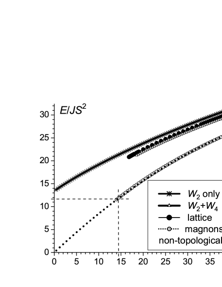
Figure 2: Dependence $E_{\rm{min}}(N)$ for topological and non-topological solitons for the case of exchange anisotropy only, $\kappa=0.2$. Dashed lines, parallel to the axes, correspond to characteristic number of bound magnons $N=N_{c}$ for non-topological soliton, see the text above. Curves, corresponding to contribution of $W_{2}$ only are shown for comparison.

Here we introduced the following notations

$$\gamma_{0}(z)=\int_{0}^{\infty}\sin^{2}\theta xdx,\quad\gamma_{2}(z)=\frac{1}{2}\int_{0}^{\infty}xdx\left[\theta^{\prime 2}\left(1+\kappa\sin^{2}\theta\right)+\frac{\sin^{2}\theta}{x^{2}}\right],$$

$$\gamma_{4}(z)=\int_{0}^{\infty}xdx\Biggl{\{}\left(\Delta_{x}\theta\right)^{2}\left(1+\kappa\sin^{2}\theta\right)+\theta^{\prime 4}\left(1+\kappa\cos^{2}\theta\right)+\frac{\sin^{2}\theta}{x^{2}}\left(\frac{1}{x^{2}}+2\theta^{\prime 2}\right)+$$

$$+\Delta_{x}\theta\sin 2\theta\left(\kappa\theta^{\prime 2}-\frac{1}{x^{2}}\right)\Biggr{\}},\ \ \theta^{\prime}=\frac{d\theta}{dx},\ \Delta_{x}\theta=\frac{d^{2}\theta}{dx^{2}}+\frac{1}{x}\frac{d\theta}{dx}\;.$$ (28)

Thus, we express the energy and the number of magnons via two parameters, $\lambda$ and $z$. It turns out, that initial dimensional variables $\Lambda$ and $R$ enter the problem only in the form of their product $z$. The dependence of $N$ and $E$ on $z$ enters the problem via a few complicated functions $\psi,\gamma_{0},\gamma_{2}$ and $\gamma_{4}$, which can be written only implicitly in the form of integrals. However, in terms of these functions, the dependence on $\lambda$ (27) turns out to be quite simple. This permits reformulation of the initial variational problem in terms of variables $z$ and $N$ only. Namely, we express

$$\lambda^{2}=4\pi\frac{z^{2}}{(N/S)}\psi(z)$$ (29)

and substitute this expression in the dimensionless energy (27). This gives us the expression for the energy of a soliton with given $N$, as a function of variational parameter $z$. Then we can find a minimum of $E$ with respect to $z$, keeping $N$ constant. The result of such minimization in the form of the dependence $E_{\rm{min}}(N)$ is shown in Fig.2 for a magnet with purely exchange anisotropy (i.e. for that with $K=0$). We show this dependence for $\kappa=0.2$. It is seen that there is a good correspondence between the dependencies $E(N)$ found by variational and numerical (full symbol) minimizations in the region of parameters where the soliton is stable. This justifies the applicability of the variational approach with the trial functions of the form (25) to the problem under consideration. The approach based on simpler trial functions $f_{2}$ reproduce well the particular feature found for numerical analysis of the discrete model; namely, the value of the threshold number $N_{\rm{cr}}$.

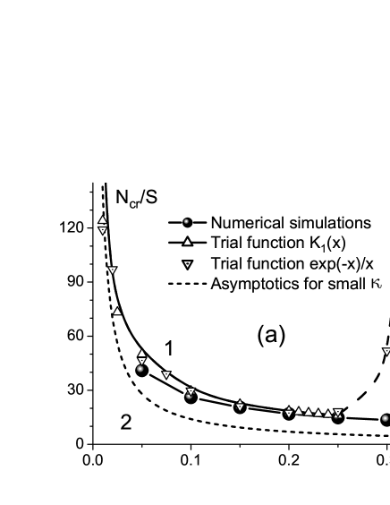
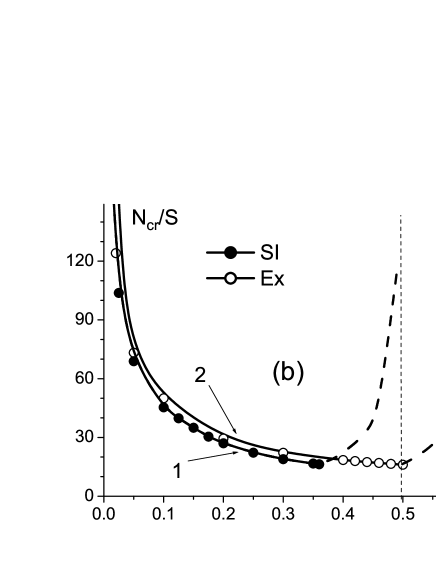
Figure 3: Soliton phase diagram. (a) - exchange anisotropy, solitons exist in the region 1 and do not exist in the region 2. For small $\kappa$ the value of $N_{\rm{cr}}\approx 1.4S/\kappa$. (b) - comparison between exchange (curve 1) and single-ion (curve 2) anisotropies. Limiting values of $N_{\rm{cr}}$ for both types of anisotropies are shown by vertical dashed lines.

Also, for comparison, we show in Fig. 2 the result of variational minimization of $W_{2}$ (i.e. energy, incorporating only squares of magnetization gradients). It is seen, that in this case there is no $N_{\rm{cr}}$, which coincides well with the previous investigations of solitons in the continuum models.Voronov83 ; Ivanov86 ; Kosevich90 This means, that mapping of the initial discrete model on the simplest continuum model with only squares of magnetization gradients can be wrong for some values an $N$, and to get the correct description of solitons in a 2D magnet one must take into account at least fourth powers of gradients. On the other hand, for large enough $N$ and even moderate value of anisotropy, the role of this higher derivative terms is less important; it is in agreement with the recent numerical simulations of soliton dynamics for easy-axial discrete models of ferromagnets Sheka+ivanov+EuJP06 .

It is seen from Fig.2, that the topological solitons in such a model are not very ”robust” - there is a quite large parameter region where those solitons are unstable or do not exist at all. That is why for comparison we show the dependence $E(N)$ for non-topological solitons (open symbols on the figure) which have been studied in detail analytically in Ref. IvZaspYastr, . The main feature of non-topological solitons is that while $\omega\to\omega_{0}$, the amplitude of such solitons diminishes (so that at $\omega\geq\omega_{0}$ such soliton decays to a number of noninteracting magnons) but both its energy $E\equiv E_{\rm NT}\approx 11.7E_{\rm BP}$ and bound magnons number $N\equiv N_{c}=E_{\mathrm{NT}}/\hbar\omega_{0}$ are left intact. IvZaspYastr This behavior is opposite to that of a topological soliton, where as $\omega\to\omega_{0}$ the amplitude still has its maximal value with decreasing soliton radius so that soliton becomes ”more localized”. This tendency is seen in Fig.2, where a non-topological soliton exists up to $N\equiv N_{NT}$ (corresponding to $\omega=\omega_{0}$, shown as vertical dotted line on the figure) and then decays smoothly into a noninteracting magnon cloud with the energy above on the corresponding curve (dotted line in the figure). This is because as $\omega\to\omega_{0}$ the non-topological soliton has the same energy as corresponding magnon cloud. But the soliton is ”coherent” (in a sense that it is a bound state of many magnons), while magnon clouds are not coherent. Actually, the above remark reflects the important point in a physics of solitons under consideration, namely the difference in behavior of topological and non-topological solitons.

As was mentioned above, there is a critical value of bound magnons number $N_{\rm{cr}}$ such that the topological soliton exists with $N\geq N_{\rm{cr}}$ only. This threshold depends on $\kappa$. This dependence, which we will call a phase diagram, is depicted in Fig.3a. The solitons exist in the region 1 above corresponding curves and do not exist in the region 2 below them. For comparison, on the same figure, we plot the points $N_{\rm{cr}}$, corresponding to different trial functions. Very good coincidence between these points shows that both trial functions are well-suited for variational treatment of the solitons.

It is seen that the threshold number of bound magnons calculated using the simple variational approach grows infinitely both for $\kappa\to 0$ and for $\kappa\to\kappa_{\rm lim}\approx 0.312$. The comparison with the numerical data shows that the divergence at the large values of anisotropy is simply an artifact of continuous description, and the corresponding “numerical” curve for discrete model decreases monotonously with growing of anisotropy. For high anisotropies, the soliton structure becomes strongly anisotropic, and the description based on radially-symmetric trial functions fails. We will discuss this in the next section.

On the other hand, the divergence of $N_{\rm{cr}}$ at small $\kappa$ has a clear physical meaning and coincides well with the numerical data. The divergence of $N_{\rm{cr}}$ at $\kappa\to 0$ is related to the fact that in BP soliton, which is the exact soliton solution for purely isotropic ferromagnet, the integral describing the value of bound magnons $N$ diverges logarithmically as $r\to\infty$ due to slow decay of the function $\theta(r)\propto 1/r$. Using the variational approach with the asymptotics of the functions (28) it is possible to derive the asymptotic formula for $N_{\rm{cr}}$ in this region, which reads

$$N_{{\rm cr}}(\kappa)\approx\frac{1.4S}{\kappa}.$$ (30)

In contrast, the critical value of energy $E_{\rm{cr}}=E(N_{\rm{cr}})$ is finite at the instability point,

$$E_{{\rm cr}}(\kappa)\approx 4\pi JS^{2}(1+2.64\sqrt{\kappa/J}).$$ (31)

This limiting energy contains non-analytical dependence on the anisotropy constant $\kappa$. It appears due to simultaneous accounting of the anisotropy and fourth derivative terms in our generalized continuum model. For typical values $\kappa/J=0.1\div 0.2$, this energy is well above the Belavin-Polyakov limiting energy, see Figs. 1, 2. The correction to $E_{BP}$ becomes smaller then 1% at extremely low anisotropies like $\kappa\leq 10^{-5}J$ only. The situation here is very similar to the analysis of heavy (less energetically favorable) vortex decay in the cone state of an easy plane ferromagnet, IvWysin02 which situation occurs in a magnetic field, perpendicular to the easy plane.IvSheka ; IvWysin02 There, in the simple continuum model, the heavy vortices are stable in the entire region of cone state existence ($0<H<H_{a}$, $H_{a}$ is an anisotropy field)IvSheka , but already for very small anisotropies $\kappa\simeq 10^{-4}$, when $l_{0}\simeq 10a$, this region has diminished substantially so that at $\kappa\simeq 0.1$ the heavy vortices have already become absent.IvWysin02

In Fig.3b, the phase diagrams for exchange (curve 1) and single-ion anisotropies (curve 2) are shown. It is seen, that while at small $\kappa$ and $K$ the corresponding curves lie close to each other, for larger anisotropies there is a drastic difference. While the (unphysical) limiting value of $N_{\rm{cr}}$ for high exchange anisotropy $\kappa$ equals 0.312, corresponding to $K_{\rm{eff}}=0.624$, the same value for single-ion anisotropy constant $K$ corresponds to $K_{\rm{eff}}\approx$ 0.5. This means that the continuous description for exchange anisotropy is valid for larger values of anisotropy constants, even in the region $K_{\rm{eff}}\simeq 0.5$, where it already fails for single-ion anisotropy. This is a consequence of the fact, that the single-ion anisotropy constant $K$ enters the problem only in the spatially homogeneous term (via the combination $K_{\rm{eff}}$, see above), while the constant $\kappa$ enters all terms of expansion $W_{i}$.

V Solitons in the discrete model with high anisotropy. Magic numbers of bound magnons

For large anisotropies, the discreteness plays a decisive role so that exact analytical treatment of the problem is impossible. However, an account for the following two facts permits to accomplish a comprehensive approximate study. First, as was mentioned in the early publications, IvKos76 ; KovKosMasl ; IvDzyal for the large number of bound magnons $N\geq S(l_{0}/a)^{2}$ , any solitons in two- and three dimensional magnets, topological and non-topological, can be presented as a finite region of flipped spins, separated by 180^∘ domain wall (DW) from the rest of a magnet.

Second, for such solitons (magnon droplets) the difference between topological and non-topological textures becomes vague. As the anisotropy grows, $l_{0}\sim a$ and the characteristic magnon number becomes comparable with $2\pi S$. At the same time, the DW becomes thinner so that at $\kappa,K\sim J$ its width becomes comparable with lattice constant $a$. It is clear that already at high anisotropy the structure of bound states (solitons) with $N/S\geq 10$ is above the described flipped area bordered by the DW (we recollect here that we consider a soliton as a bound state of many magnons) so that the soliton properties will be completely determined by those of the DW. It is also clear that for this case the difference between topological and non-topological solitons will be negligible. We will see, that in this case the structure of bound state is strongly dependent on the character of anisotropy. That is why for a description of such bound states it is useful to study first the structure and properties of the DW’s in highly anisotropic 2D magnets with different types of anisotropy. First of all, of importance is a notion of the DW pinning, i.e. the dependence of its energy both on the DW center position in a lattice (positional pinning) and on its orientation with respect to the lattice vectors (orientational pinning).

The positional pinning of a DW can be discussed on the basis of a simple 1D model of a spin chain. This case is obviously applicable to the 2D square lattice with nearest-neighbor interaction for the DW orientation along lattice diagonals (the directions of (1,1) type). For a chain, it is natural to associate the DW coordinate $X$ with the total spin projection on the easy axis ${\cal S}_{tot}^{z\ (0)}$ and to define it as follows IvMik . Let us choose some lattice site and define the DW located on this site to have the coordinate $X=0$. Let us then determine the coordinate of any DW via its total spin $z$-projection ${\cal S}_{tot}^{z}$ from the expression

$$X=\frac{a}{2S}\sum_{n=-\infty}^{n=\infty}[S^{z}_{n}(X)-S_{n}^{z}(X=0)],$$ (32)

where $S_{n}^{z}(X=0)$ defines the spin distribution in a DW at a reference point $X=0$.

For the solitons description, the different properties of DW placed in different positions play a crucial role. First, consider a DW in a middle between two arbitrary lattice sites, for which $X/a$ is half-odd, $X=a(2n+1)/2$. Only domain walls of such type in the highly anisotropic magnet can be purely collinear, i.e. it may have $S_{z}=\pm S$, respectively, on the left and right sides of the DW center. For the case of a spin chain with single-ion anisotropy this is achieved for $K>0.5$,Kovalev+ which was associated with the destruction of non-collinear topological structure Kamppeter01 . According to the definition (32), it is a vital necessity to have a non-integer ${\cal S}_{tot}^{z}$ and non-collinear component for the rest of the DW positions. For example, for $X=(a/2)(2n)$ in the one of the sites $S_{z}=0$, i.e. $\theta=\pi/2$.

The question regarding the character of the pinning potential $U(X)$ is also important. Gochev has shown, that there is no pinning, i.e. $U=0$, in a spin chain with purely exchange anisotropy.Gochev On the other hand, for the anisotropy of a pure single-ion type, the potential $U(X)$ has minima in the points of type $a(2n+1)/2$, which favors the appearance of collinear DW’sIvMik . For the small perturbation of a problem with exchange anisotropy by single-ion anisotropy with negative sign $K<0$, it turns out that $U(X)$ has the minimum at integer values of $X/a$, $X=0$, $\pm a,\ ...$, i.e. the creation of a non-collinear structure becomes favorable. The detailed investigation of the character of DW pinning for general models with combined anisotropy shows, hoverer, that this situation is mostly an exception and the intensity of such pinning is never large. The pinning potential for the parameters where it has minima at integer $X/a$ is much smaller (at least one order of magnitude) than that for pure single-ion anisotropy.

Thus, for the two above mentioned cases one can expect substantially different spin distributions in a soliton boundary. In particular, DW pinning on lattice sites can yield the conservation, at least partial, of a soliton topological structure even with strong discreteness effects. On the other hand, a DW pinned between lattice cites becomes collinear and hence its topological structure can be easily lost.

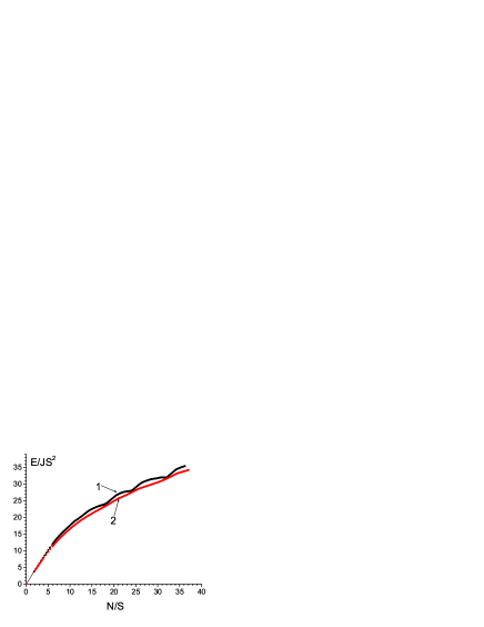
Figure 4: Dependence $E(N)$, obtained by numerical simulations for $K_{\rm{eff}}=1$. Curve 1- single-ion, $K=1$, curve 2 - exchange, $\kappa=0.5$.

It is clear, that for the question about the structure of a closed soliton boundary, the important point is its angular pinning, i.e. the dependence of the planar DW energy on its orientation in a crystal. Gochev suggested, that the optimal DW direction is parallel to the primitive vectors of lattice translation, (1,0) and (0,1),Gochev that differs from the conclusions of Ref. Kamppeter01, . Our analysis has shown that almost all numerical data about the properties of the solitons in highly anisotropic FM’s can be described under supposition that a DW tends to be parallel to (0,1) direction. As we shall show, only $N/S$ is a main parameter determining the soliton structure at high magnetic anisotropy. It turns out that the variation of $N/S$ by around few percent yields substantial variations of DW structure, which leads to sharp dependence of energy $E$ (see Fig.4) and particularly the frequency $\omega$ on $N$, see Fig. 7 below. This effect is different for single-ion and exchange anisotropies, the most substantial manifestation is for the single-ion case. These dependencies have a non-monotonic component. Its analysis reveals certain specific numbers $N_{\rm{mag}}$, which, analogously to nuclear physics, can be called the magic numbers. To explain the origin of these magic numbers, we consider the case when a DW tends to occupy a position between atomic planes of (1,0) and/or (0,1) type so that both DW bend and non-collinear structure formation are unfavorable. Then, the optimal (from the point of view of DW energy) configuration, is that where the spins with $S_{z}=-S$ occupy a rectangle $l_{x}\cdot l_{y}$, separated from the rest of a magnet by a collinear DW. Clearly, the most favorable configuration is that with spin square $l_{x}=l_{y}$, which yields $N_{\rm{magic}}=2l^{2}S$, but configurations with $l_{x}\approx l_{y}$, like those having $N/S=2\cdot(l)(l+1)$, for example, $N/S=2\cdot(3\cdot 4)=24$ are also quite profitable, see Fig. 4. We will call such values of $N$ half-magic. As we shall see, such a model describes the solitons in magnets with single-ion anisotropy for $N/S=15\div 50$ pretty well. If the energy of spatial and angular pinnings is not so important, we may expect more or less cylindrical shape of a soliton core and smooth dependencies $E(N)$ and $\omega(N)$. The numerical analysis has demonstrated, that both above tendencies reveal themselves in a FM with single-ion and exchange anisotropies respectively, see Fig. 4 for $E(N)$ dependence. Namely, for SIA the dependence $E(N)$ has a non-monotonous component, while for ExA this dependence seems to be more regular. The minima in the non-monotonous dependence $E(N)$ for SIA occur for $N/S=18$ $=2\cdot 3^{2}$, $24=2(3\cdot 4)$ and $32=2\cdot 4^{2}$. Hence, the above magic and half-magic numbers, related to the DW pinning between two atomic planes, are clearly seen in the $E(N)$ dependence.

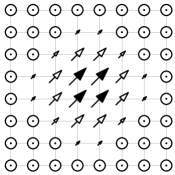
(a) ExA, 8

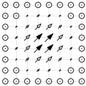
(b) SIA, 8

(c) ExA, 12.

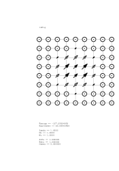
(d) SIA, 12.

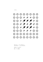
(e) ExA, 14.

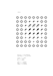
(f) SIA, 14

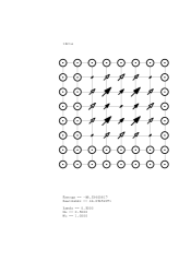
(g) ExA, 18.

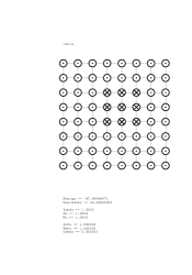
(h) SIA, 18.

Figure 5: The structure of the soliton textures for the magnets with exchange (left column) and single-ion anisotropy (right column) with the same value of effective anisotropy and different values of $n=N/S$ (shown as subfigure captions). The arrows present in-plane spin projections in 20 by 20 lattice. ”Up” ($0\leq\theta\leq 10^{\circ}$) and ”down” ($170^{\circ}\leq\theta\leq 180^{\circ}$ ) spins are presented by dotted and crossed circles, respectively. The in-plane projections of the spins with ”up”  and ”down”  $z-$ projections are depicted by arrows with open and full heads, respectively.

We now discuss non-topological spin configurations for different numbers of bound magnons for ferromagnets with single-ion and exchange anisotropy with large value of effective anisotropy constant $K_{\rm{eff}}=J$, see Figs.5 and 6. Let us first consider the small values $n\equiv N/S<20$. To economize the notations, hereafter we will use $n$ instead of $N$. For very small $n<10$ the soliton textures have the same noncollinear structure for both types of anisotropies, SiA and ExA, see Figs. 5(a),5(b). The difference between spin textures for SIA and ExA solitons becomes visible for $n\geq 10$. In this case, the effects of lowering of a soliton symmetry with respect to expected lattice symmetry of fourth order C₄, are possible. For half-magic number $n=12$, corresponding to collinear texture with flipped spins rectangle $2\times 3$, the symmetry C₄ is obviously absent both for SIA and for ExA, see Figs. 5(c),5(d). Also, there is no big difference between spin textures in Figs. 5(c),5(d). However, for $n$ far from magic numbers, the difference between SIA and ExA is much more pronounced. In particular, for the SIA case there is not even a C₂ axis (Fig. 5(f)), while for ExA, the C₄ symmetry is restored (Fig. 5(e)). The explanation is pretty simple: the DW pinning is weaker for ExA then that for SIA so that in former case the symmetric closed DW is formed, while for SIA more favorable is the formation of a piece of “unfavorable” DW, occupying only the part of a soliton boundary, which makes possible optimization of DW structure for the rest of the boundary. As $n$ increases further for SIA the purely collinear structures of the above discussed type, can appear, see Fig.5(h),6(j). As for the ExA case, even at sufficiently large $n=32$, the soliton texture does not contain a purely collinear DW, see $n=18$ in Fig.5(g) and large $n=32$ in Fig.6(i) below.

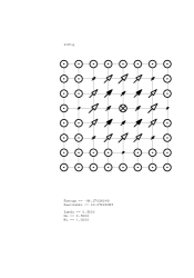
(a) ExA, 21.

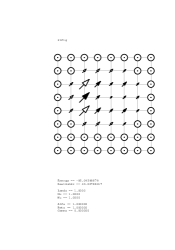
(b) SIA, 21.

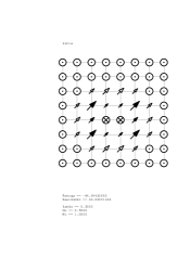
(c) ExA, 24.

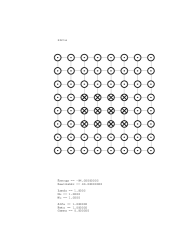
(d) SIA, 24.

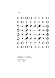
(e) ExA, 28.

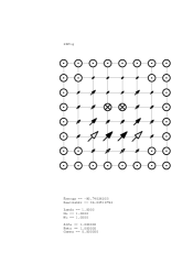
(f) SIA, 28.

(g) ExA, 31.

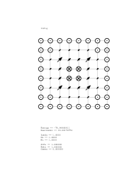
(h) SIA, 31.

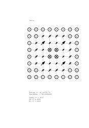
(i) ExA, 32

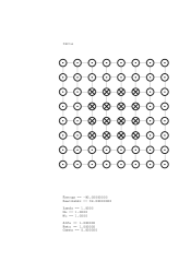
(j) SIA, 32.

Figure 6: The same as in Fig. 5 for larger values of $n$.

Thus, at small $n$, the certain tendency, which is confirmed at large $n$ (see Fig. 6), is clearly seen. Namely, the strong DW pinning for the SIA case yields almost always the nonsymmetric configurations, where $n$ growth occurs due to increase or decrease of “DW pieces” on a soliton boundary, Figs.6(b),6(f). The exceptions are magic numbers $n_{\rm mag}=2l^{2}$ (Figs. 5(h),  6(j)) or close to them “half-magic” numbers $n_{\rm hm}=2l(l+1)$ (Fig. 6(d)), where the collinear structure of the flipped spins square or rectangle type (with symmetries, respectively, C₄ and C₂) is present in SIA case. For the ExA case the numbers $n_{\rm mag}$ and $n_{\rm hm}$ are also revealed, but in a quite different manner. Namely, for $n=n_{\rm mag}$ the soliton does not have a collinear structure but resembles a square, see Fig. 6(a). Here, however, there is a fundamental difference with the SIA case. The same structures with C₄ symmetry are formed also for $n$ non-magic, $n\neq n_{\rm mag}$, $n_{\rm hm}$. This becomes clear if we recollect that in this case the pinning is weak (see above) so that “DW piece” formation is absolutely unfavorable. This means that C₄ symmetry occurs both for $n$ magic and nonmagic, see Fig.5(g),6(i). However, for $n$ half-magic, the rectangular shape of a soliton core occurs also for ExA both for small (Fig. 5(c)) and large $n$ (Fig. 6(c)). Thus, the soliton structure for the ExA case also depends on $n$ nonmonotonously, but here the “half magic” numbers are more important since close to these numbers the soliton symmetry first lowers from C₄ to C₂ and then it restored back to C₄. At the magic number $n=32$, see Figs. 6(i) and 6(j) as well as near this magic number, both SIA and ExA textures have quite symmetric structure with almost collinear DW, see Figs. 6(g) and 6(h) for $n=31$.

This complex and irregular picture of soliton behavior ”maps” onto the $E(N)$ dependence only as a local energy lowering at $n\approx n_{\rm mag}$. The irregular behavior of soliton characteristics is revealed much more vividly in the dependence $\omega(N)$, seen in Figs. 7(a),(b). For both types of anisotropy, the explicit traces of nonmonotonous behavior like jumps, regions with $d\omega/dN>0$, and even those with $\omega<0$ (for SIA, see Fig 7) occur. At this point it is useful to make two remarks. First, we recollect, that for discrete systems, contrary to the continuous ones, the condition $d\omega/dN<0$ is no more a soliton stability criterion. Second, the condition $\omega<0$ just means that in this region of parameter values, the soliton energy decreases as $N$ increase, but says nothing about the soliton stability. It is seen from Fig 7(a), that the non-monotonous structure of the corresponding $\omega(N)$ curves manifests itself most vividly at $n>10\div 15$. For SIA, the abrupt vertical up and downward jumps with growing of $n$ on the curve $\omega(N)$ appear at certain values of $n$. The upward jumps occur near magic and half-magic numbers introduced above. After these upward jumps, the frequency has plateaus at $18<n<20$, $24<n<26$, $32<n<34$, and then the deep minima. For large $n\sim 31\div 32$, the frequency becomes negative, $\omega<0$. The fact, that these negative values occur only for SIA for $n$, slightly less then the “magic” value $n=32$, corroborates the above suggested concept.

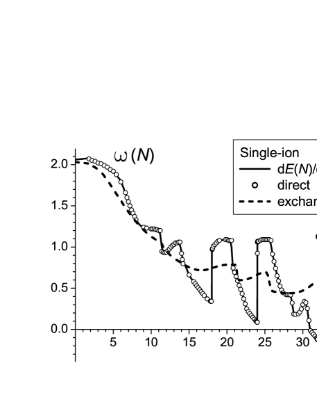
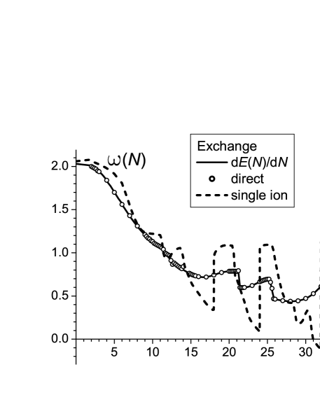
Figure 7: Dependence $\omega(N)$ for a soliton with $K_{\rm{eff}}=J$, obtained from numerical simulations. (a)- Single ion anisotropy, (b) - exchange anisotropy. Dashed lines are for better comparison and correspond to exchange anisotropy (a) and single ion one (b).

For the case of exchange anisotropy (Fig.7b), the upward jumps on the curve $\omega(N)$ are almost absent, and the smooth increase of $\omega$ occurs instead, i.e. the effect of ”magic” numbers is absent. The downward jumps are clearly seen at the same values of $n$ as those for SIA. These jumps sometimes are much sharper that those for SIA, but for ExA the amplitude of these jumps are smaller, than for SIA, and $\omega>0$ everywhere.

The physical explanation of the above quite complicated behavior can be done based on the aforementioned picture. First, the upward jumps for $n=n_{\rm mag}$ with subsequent almost constant $\omega$ can be easily understood for SIA. In this case, at $n=n_{\rm mag}$ the formation of favorable collinear structure has already been finished so that the plateau at larger $n$ is due to the creation and growth of a ”DW piece”. It is clear that for ExA this scenario does not occur, and this effect is completely absent. The downward jump and general decrease of the soliton frequency is related to the transition to more symmetric configurations, where the excessive number, $n$ of magnons is easily spread along the soliton boundary. Such transitions take place for both types of anisotropies, which explains the behavior similarities.

Let us discuss now the possibility of the topological soliton existence in high anisotropy ferromagnets. In this specific case, it is useful to utilize a simplified obvious definition of the topological invariant. The $\pi_{2}$ topological invariant (12) for the case of large anisotropy has simple geometric meaning. Namely, only $\theta\neq 0,\pi$ make a contribution into integral (12) so that for its evaluation it is sufficient to consider the DW region. Formally, the integral (12) can be represented as a contour integral along the DW,

$$Q\to\frac{1}{2\pi}\oint\frac{\partial\phi}{\partial\chi}d\chi.$$

This value defines a mapping of the DW line (which is of necessity a closed loop) onto the closed contour which is a domain of angle $\phi$ variation. This representation makes it obvious that the topological charge, $Q$ notion is meaningful only in the case when the DW has a well defined noncollinear structure throughout its length. The DW regions with collinear spins play the role of a ”weak link”, where $\phi$ can change abruptly by $2\pi$ almost without overcoming the potential barrier. Hence, even for nonsymmetric soliton textures, when soliton has a quite large ”piece” of noncollinear DW, with ”quasitopological”  spin inhomogeneity, literally topological structures are absent. Although the difference between topological and nontopological solitons in the magnets with $K_{\rm eff}\sim J$ is not that large and the question about realization of topological solitons in such structures is rather academic, this problem will be discussed in more details.

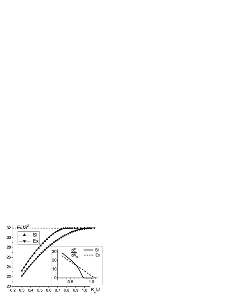
Figure 8: The energy of the soliton with $N/S=32$ (magic) as a function of effective anisotropy constant. Inset shows the behavior of a derivative $dE/dK_{\rm{eff}}$ near $K_{\rm{crit}}\approx 0.8$.

To answer the question about the presence or absence of a topological texture, we have carried out the numerical minimization both over a complete set of variables and over $\theta$’s only with fixed in-plane spin directions. Contrary to the above considered case of moderate anisotropy, the latter minimization (i.e. that over $\theta$’s only) never gives the instability of a nontrivial topological structure. Instead, the decrease of noncollinear structure amplitude (either uniformly along the entire DW or on its individual parts) occurs as $K_{\rm{eff}}$ increases. The behavior is quite different for different values of $n=N/S$ so that these cases should be considered separately. For specific analysis, we have chosen a few $n$ values, typical ”magic” number $n=32$ and two non-magic, $n=35$ and $n=36$. In spite of closeness of these numbers, the soliton spin texture behavior in these cases differs drastically as anisotropy increases.

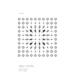
(a) ExA, 0.6

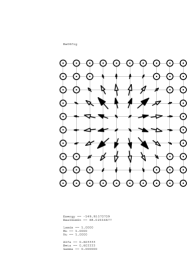
(b) SIA, 0.6

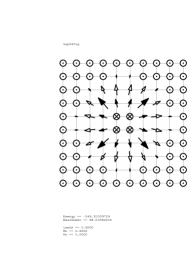
(c) ExA, 0.8

(d) SIA, 0.8

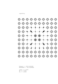
(e) ExA, 1.0

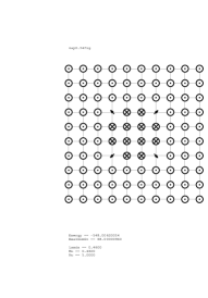
(f) ExA, 1.08

Figure 9: Soliton structure for magic number of bound magnons $N=32S$ and different values of effective anisotropy constant $K_{e}$, the value of $K_{e}/J$, together with the type of anisotropy, are shown below pictures of spin distribution.

The energy of the topological soliton as a function of $K_{\rm{eff}}/J$ for magic number $n=32$ and two types of anisotropy is shown in Fig.8. These curves have been obtained by numerical simulations on a lattice, for an anisotropy increase from its small value, when there is a well-defined topological soliton texture. It is seen that at large $K_{\rm{eff}}$ the soliton energy tends to some finite limiting value, $E_{0}=32JS^{2}$, that is typical for a collinear structure with the “magic number” $n=32$. But the behavior of these functions near this limiting value is different for single-ion and exchange anisotropies, corresponding to the different scenarios of annihilating of both non-collinear spin structure and topological structure in a soliton. It is interesting to trace the disappearance of a soliton topological structure at anisotropy increase, which is shown in Figs. 9. For small $K_{\rm{eff}}$ the topological structure is well defined, and this structure is similar for both SIA and ExA, see Figs. 9(a) and 9(b). If the value of $K_{\rm{eff}}$ increases to some critical value, $K_{\rm{crit}}$, the in-plane spin amplitude decreases, but a “vortex-like” configuration with approximate symmetry C₄ is still visible. For larger anisotropy $K\geq K_{\rm{crit}}$ the soliton structure becomes purely collinear. For SIA the critical value is $K_{\rm{crit}}\approx 0.8$, but for ExA this value is much larger, $K_{\rm{crit}}\approx 1.1$, compare Figs. 9(d) and 9(c). For ExA, the topological structure is still visible for such strong anisotropy as $2\kappa=K_{e}=J$, see Fig. 9(e). However, for high enough $\kappa$ the structure finally becomes collinear and of the same structure as that for SIA, as is shown in Fig. 9(f). In other words, for “magic” magnon numbers the topological structure of a soliton decays smoothly as the anisotropy constant grows, which is seen for both types of anisotropy, compare Figs. 9(d) and  9(f).

For $K_{\rm{eff}}>K_{\rm{crit}}$ for both kinds of anisotropy there is no more topological spin structure - all spins are directed either up or down and energy does not depend on $K_{\rm{eff}}$ any more (see Fig.8). Such a picture resembles very much the phase transition of a second kind with the collinear soliton texture as more symmetric phase. This agrees with the behavior of the energy $E(K_{\rm{eff}})$ near $K_{\rm{crit}}$, (see inset to Fig.8)

$$E-E_{0}\propto(K_{\rm{crit}}-K_{\rm{eff}})^{2}.$$ (33)

To understand better the picture of the transition from a topological (noncollinear) soliton texture to a collinear texture, we discuss the analogy with the second order phase transition in more detail. Note, that any collinear spin structure with arbitrary positions of “up” and “down” spins has the same symmetry element, namely, rotation about the $z$ - axis in a spin space. This symmetry is due to the symmetry of the Hamiltonian (II). On the other hand, the spin textures, even noncollinear, with $n=32$ and C₄ symmetry, are invariant with respect to a rotation by $(\pi/2)\cdot k$, $k\in\mathbb{Z}$, simultaneously in spin space and coordinate space. Thus, “magic” collinear textures with spatial symmetry C₄ have higher symmetry, being invariant relative to the independent rotation of the coordinate space by $(\pi/2)\cdot k$ and of the spin space by arbitrary angle, while noncollinear “magic” ones are invariant only relatively to simultaneous rotation by $(\pi/2)\cdot k$ in spin and coordinate spaces. This means that on a transition from a “magic” collinear soliton to noncollinear one, spontaneous symmetry breaking occurs and phase transition of the second kind appears naturally.

For “non-magic”  numbers $n=35$ and $n=36$, the symmetry of soliton structures and their behavior is fundamentally different. First, note that the collinear structure can be realized for even values of $n$ only. For any non-even $n$, odd-integer or non-integer, some spins have to be inclined to the $z-$axis. Thus, these two cases have to be considered separately.

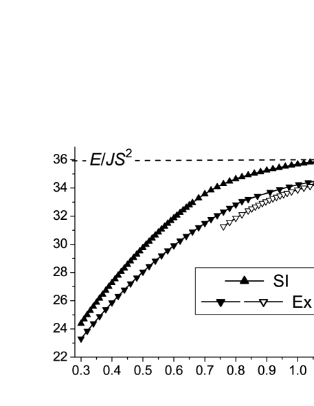
Figure 10: The energy of the soliton with $N/S=36$ (non-magic, even) as a function of effective anisotropy constant $K_{\rm{eff}}$. For exchange anisotropy, full symbols presents data for topological solitons, open symbol non-topological solitons with $Q=0$. The values of $K_{\rm{eff}}\approx 1.13$ for the transition from non-collinear to collinear soliton for single ion anisotropy are shown by vertical dotted lines.

The value $n=36$ is rather far both from ”magic” number $n=32$ and from the nearest ”half-magic”  $n=40$, corresponding to the favorable configuration with a rectangular collinear DW. Here, for small anisotropy $K_{\rm{eff}}\lesssim 0.6J$ we see the structure with C₄ symmetry, similar to that for “magic” $n=32$ for both types of anisotropy, see Fig. 9(a) and 9(b). However, with the increase of $K_{\rm{eff}}$, the evolution is different, as seen in Fig. 10. The difference in behavior of $E(K_{\rm{eff}})$ is the largest for exchange anisotropy, where the saturation, depicted in Fig. 8, did not occur up to quite large $\kappa\gtrsim 0.6J$ ($K_{\rm{eff}}\gtrsim 1.2J$). However, for single ion anisotropy there is also a difference from the above considered “magic” case $n=32$.

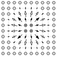
(a) ExA, 0.7

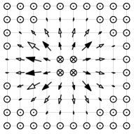
(b) SIA, 0.7

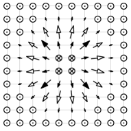
(c) ExA, 0.8

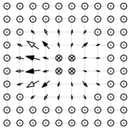
(d) SIA, 0.8

(e) ExA, 1.0

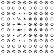
(f) SIA, 1.0

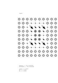
(g) ExA, 1.2

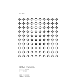
(h) SIA, 1.2

Figure 11: Soliton structure for N=36 (even non-magic number) and different values of effective anisotropy constant $K_{e}/J$ (shown in captions)

Those differences could be explained in terms of previously discussed fact that DW pinning is stronger for SIA compared to ExA. Using symmetry arguments, we note that the purely collinear texture for $n=36$ has a DW of complex form, lower symmetry (Fig.11(h)), and is much less energetically favorable, than that for $n=32$. Hence, this state in its pure form occurs only for sufficiently large SIA with $K>1.18J$ rather then for $K>0.8J$ as for the ”magic”  case $n=32$. We have found that the textures with sufficiently high symmetry (in any case they have a center of symmetry or a couple of C₂ axes) are inherent to exchange anisotropy. Such textures for non-magic $n$’s have DW’s of strong non-collinear structure with a great number of spins with $\theta\simeq 90^{\circ}$. For the ExA case, the DW does not ”tear apart” up to quite large $\kappa>0.5J$ ($K_{\rm{eff}}\gtrsim J$). Here both topological and non-topological soliton textures exist. The energy of latter textures is shown in Fig. 10 by open symbols. For $\kappa\lesssim 0.4$ both types of solitons have a rectangular shape and rather high symmetry. Their difference is that for non-topological soliton the inversion center is present even for $K_{\rm{eff}}\simeq 1.2J$ while the symmetry of a topological soliton lowers already for $K_{\rm{eff}}\simeq J$, see Fig. 11(e),11(g). This difference can be understood as follows. For a topological soliton, the DW containing spins with $\theta\simeq 90^{\circ}$ (since the spin angle $\phi$ is inhomogeneous) is less favorable than that for non-topological solitons. Thus, for topological solitons the spins with $\theta\neq 0,\pi$ concentrate near one of the soliton edges. However, the energy difference of these solitons at $K_{\rm{eff}}>1.1J$ is quite small. Thus we may assert that in the wide range of ExA constants we have two soliton types with similar structure of spins along the easy axis and approximately equal energies.

In the SIA case the DW pinning plays a much more important role so that the low symmetry, which is characteristic of collinear texture of the type shown in Fig.11(h), can be traced already for sufficiently small $K_{\rm{eff}}\gtrsim 0.7J$, see Figs.11(d),11(f). Since the DW inhomogeneity, caused by a topology, is localized in a small part of a boundary, its role is not essential so that there is no big difference between topological and non-topological solitons. At least this difference is much less pronounced than that for ExA where the non-collinearity amplitude decreases smoothly as $K$ increases. The new element of symmetry (a rotation in a spin space) appears in a transition to the collinear state at $K_{\rm{eff}}\geq K_{\rm{crit}}$. That is why this transition resembles the phase transition of a second kind. This behavior of $E(N)$, similar to that for “magic” magnon numbers, can be seen in Fig. 10 for SIA (but not for ExA!).

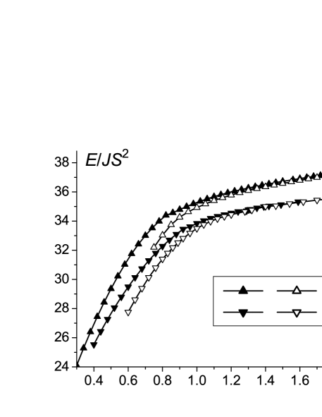
Figure 12: The energy of the soliton with $N/S=35$ (non-magic, odd) as a function of effective anisotropy constant. Full symbols present data for topological solitons with inhomogeneous DW, open symbols correspond to non-topological solitons with $q=0$.

As we have found out in the above example of $n=32$ and $n=36$, the final stage of evolution of a soliton with even $n$ is a collinear structure. Since the transition of a soliton into a collinear state is related to the symmetry increasing, it formally resembles a transition of the second kind. The collinear structure cannot be realized, for obvious reasons, for any $n$, which is not even. In this case, which has been considered for $n=35$, the smooth variation of a soliton energy and structure occurs, see Fig. 12. In particular, its energy is a monotonously increasing function of $K_{\rm{eff}}$ for both types of anisotropies. For high enough anisotropy, the difference between topological and non-topological solitons diminish.

VI Conclusions

In this paper we have studied the topological and non-topological solitons, stabilized by precessional spin dynamics in a classical 2D ferromagnet with high easy–axis anisotropy on a square lattice. Our analysis has been performed both analytically in the continuous approximation and numerically. The main conclusion is, that in the 2D case the solitons properties change drastically upon departure from the ”singular point” - isotropic continuous model with BP solitons. Similar to previous studies, it turns out that the presence of even weak anisotropy makes solitons dynamic, i.e. those with nonzero precession frequency for any number $N$ of bound magnons. It is very interesting and unexpected, that the role of discreteness turns out to be of the same importance as that for anisotropy, even for $\kappa$, $K\ll 1$, when $l_{0}\gg a$. The minimal consideration of discreteness (via higher degrees of gradients) yields the existence of some critical value (lower threshold) of both soliton energy and the number of bound magnons. Similar to the problem of cone state vortices, the instability is related to the joint action of discreteness and anisotropy ”responsible” for $l_{0}$ formation (see Eq. (14)). As a result, the nonanalytic, instead of linear, dependence of the critical soliton energy (31) on the anisotropy constant appears.

On the other hand, for intermediate values of anisotropy, like $K_{\mathrm{eff}}<(0.25\div 0.3)J$, and for the values of $N$ far enough from the critical value of the bound magnons $N_{\mathrm{cr}}$, we have checked and confirmed a number of results regarding soliton structure from the continuous theory. In particular, the relation between the number of bound magnons and precession frequency of spins inside the soliton is common to these two approaches. In agreement with Ref. IvZaspYastr, non-topological solitons have, as a rule, the lower energy than the topological ones (see Fig.1), and they are stable for any $N>N_{NT}$.

Some fundamentally new features in soliton behavior appears as the anisotropy grows. For ”magic” numbers of bound magnons, $N=2l^{2}S$, $l$ is an integer, the soliton texture corresponds to the most favorable structure with a collinear DW of a square shape. In this case the soliton topological structure disappears (as anisotropy grows) continuously (to some extend analogously to the second order phase transition) giving purely collinear state. Such behavior is inherent to both types of anisotropy, but for SIA the critical value $K_{\rm{crit}}$ is lower and the transition is sharper. For non-magic numbers, when the collinear structure is certainly less favorable, it still appears for even numbers $N/S$ and the SIA case by a smooth transition, but with essentially larger $K_{\rm{crit}}$. Note that in all cases this value of $K_{\rm{crit}}$ is much larger then that for 1D spin chain, $K_{\rm{crit}}^{(1D)}=0.5J$ Kamppeter01 ; Kovalev+ . Finally, if $n$ is not an even number, then for $K\gtrsim J$ the soliton always has a non-collinear structure in the form of DW ”piece” or even a single spin with $S_{z}\neq\pm 1$. The energy of such a soliton is almost independent of inhomogeneity of planar spin components in the DW.

Let us note one more interesting property of the solitons in magnets with strong anisotropy, namely the existence of the stable static solitons in this case. It is widely accepted, that such solitons are forbidden both in the model with $W_{2}$ (Hobart-Derrick theorem) and in the generalized model with negative contribution of fourth powers of magnetization gradients ($W_{2}+W_{4}$ in this article). However, the region of $N$ values, where the soliton frequency changes its sign, is clearly seen on the Fig. 7 for SIA. This means the existence of certain characteristic values of $N$, where $\omega=0$ and the soliton is actually static. Also, for given number of $N$ in some region one can find the corresponding value of anisotropy constant (high enough) to fulfill the condition $\omega=0$ and to realize this static soliton with non-collinear state. In addition, all purely collinear configurations, existing for sufficiently strong anisotropy of both types, are indeed static since the precession with the frequency $\omega$ around the easy axis does not define any actual magnetization dynamics. Hence, in the magnets with sufficiently strong anisotropy the stable static soliton textures can exist. But, contrary to Ref. Ivanov86, , they are due to discreteness effects, namely due to DW pinning.

To finish the discussion of the problem considered in this work, let us consider the effects taking place at the transition from classical vectors $\vec{S}_{\vec{n}}$ to quantum spins. Usually the simple condition of integrity of the total $z$-projection of spin $N$, see (15), is considered as a condition of semi-classical quantization of classical soliton solutions of Landau-Lifshitz equation for uniaxial ferromagnets Kosevich90 . Moreover, the dependence $E=E(N)$ is used to be interpreted as a semiclassical approximation to the quantum result. Note, that for some exactly integrable models, for example, $XYZ-$ spin chain with spin $S=1/2$, the exact quantum result coincides with that derived from the semi-classical approach, see Ref. Kosevich90, ). This simple picture was elaborated for solitons having the radial symmetry. Now we consider how this picture may be modified for solitons with lower spatial symmetry discussed in this article. Solitons with low enough symmetry, say ”rectangular” solitons for ”half-magic” numbers, or even lower symmetry, which occurs for ”non-magic” numbers and especially odd ones, apparently occur for high-anisotropy magnets. It is clear, that they can be oriented in a different way in a lattice, that may be construed as $k$-fold degeneracy of a corresponding state in the purely classical case, with $k=2$ for a ”rectangular” soliton or $k>2$ for less symmetric states like those reported in the Fig. 11. With the account for effects of coherent quantum tunneling transitions between these states, this degeneration should be lifted. According to the semiclassical approach, valid for bound states of a large number of spin deviations in high anisotropy magnets, the transition probability is low and can be calculated using instantons concept with Gaussian integration over all possible instanton trajectories MQT . As a result one can expect the splitting of states degenerated in the purely classical case, with creation of k-multiplet and lifting of the symmetry of the soliton. A detailed discussion of these effects is beyond the scope of the present work.

This work was partly supported by the grant INTAS Ref.05-8112. We are grateful to the Institute of Mathematics and Informatics of Opole University for generous computing support.

References

- (1) A.M. Kosevich, B.A.Ivanov and A.S. Kovalev, Phys. Rep. 194, 117 (1990).
- (2) V. G. Bar’yakhtar and B. A. Ivanov Soliton Thermodynamics of low–dimensional magnets. Sov. Sci. Rev. Sec.A. 16, 3 (1993).
- (3) V. G. Bar’yakhtar, M. V. Chetkin, B. A. Ivanov and S. N. Gadetskii. Dynamics of Topological Magnetic Solitons. Experiment and Theory. (Springer–Verlag, Berlin, 1994).
- (4) C.E. Zaspel and J.E. Drumheller, International Journal of Modern Physics 10, 3649 (1996).
- (5) F. G. Mertens and A. R. Bishop, Dynamics of Vortices in Two–Dimensional Magnets. in Nonlinear Science at the Dawn of the 21th Century, edited by P.L. Christiansen, M.P. Soerensen and A.C. Scott (Springer–Verlag, Berlin, 2000).
- (6) V. L. Berezinskii, Sov. Phys. JETP 34, 610 (1972).
- (7) J. M. Kosterlitz and D. J. Thouless J. Phys. C 6, 1181 (1973).
- (8) F. G. Mertens, A. R. Bishop, G. M. Wysin and C. Kawabata Phys. Rev. B39, 591 (1989).
- (9) D. D. Wiesler, H. Zabel and S. M. Shapiro Physica B 156–157, 292 (1989).
- (10) A. A. Belavin and A. M. Polyakov, Sov. Phys. JETP Letters 22, 245 (1975).
- (11) G. E. Volovik and V. P. Mineev, Sov. Phys. JETP 45, 1186 (1977); N. D. Mermin, Rev. Mod. Phys. 51, 591 (1979)
- (12) H. Walliser and G. Holzwarth, Phys. Rev. B61, 2819 (2000).
- (13) R.E. Prange and S.M. Girvin, eds., The quantum Hall effect (Springer, New York, 1990).
- (14) Ian Affleck, J. Phys.: Condens. Matter. 1, 3047 (1989); I. Affleck, in: Fields, Strings and Critical Phenomena [ed. E. Brézin and J. Zinn-Justin, North-Holland, Amsterdam, 1990], p. 567.
- (15) R.H. Hobard, Proc. Phys. Soc. 82, 201 (1963).
- (16) G.H. Derrick, J. Math. Phys. 5, 1252 (1964).
- (17) V.G. Makhankov, Phys. Rep. 35, 1 (1978).
- (18) B. A. Ivanov, C.E. Zaspel and I.A. Yastremsky, Phys. Rev. B63, 134413 (2001).
- (19) F. Waldner, Journ. Magn. Magn. Mater. 31–34, 1203 (1983); ibid. 54–57, 873 (1986); ibid. 104–107, 793 (1992).
- (20) C. E. Zaspel, T. E. Grigereit, and J. E. Drumheller, Phys. Rev. Lett. 74, 4539 (1995); K. Subbaraman, C. E. Zaspel and J. E. Drumheller, Phys. Rev. Lett. 80, 2201 (1998); K. Subbaraman, C. E. Zaspel and J. E. Drumheller, J. Appl. Phys. 81, 4628 (1997).
- (21) M. E. Gouvea, G. M. Wysin, S. A. Leonel, A. S. T. Pires, T. Kamppeter, and F. G. Mertens, PRB 59, 6229 (1999).
- (22) B.A. Ivanov, A.K. Kolezhuk and G.M. Wysin, Phys. Rev. Lett. 76, 511 (1996).
- (23) B. A. Ivanov and G. M. Wysin, Phys. Rev. B65, 134434, (2002).
- (24) B. A. Ivanov and D.D. Sheka, Low Temp. Phys. 21, 881 (1995).
- (25) J. B. Torrance (Jr), M. Tinkham, Phys. Rev. 187, 587 (1967); ibidem, p. 595; D. F. Nikoli, M. Tinkham, Phys. Rev. B9, 3126 (1974)
- (26) B.A. Ivanov and V.A. Stephanovich, Sov. Phys. JETP 64, 376 (1986).
- (27) V.P. Voronov, B.A. Ivanov and A.M. Kosevich, Sov. Phys. JETP 84, 2235 (1983).
- (28) T.H. Skyrme, Proc. R. Soc. London A 260, 127 (1961).
- (29) R.H. Hobard, Proc. Phys. Soc. 85, 610 (1965).
- (30) U. Enz, J. Math. Phys. 18, 347 (1977).
- (31) U. Enz, J. Math. Phys. 19, 1304 (1978).
- (32) A. A. Zhmudskii and B. A. Ivanov, JETP Lett. 65, 945 (1997).
- (33) T. Kamppeter, S. A. Leonel, F. G. Mertens, M. E. Gouvêa, A. S. T. Pires and A. S. Kovalev, Eur. Phys. J. B 21, 93 (2001).
- (34) D.D. Sheka, C. Schuster, B.A. Ivanov, and F.G. Mertens, Eur. Phys. J. B 50, 393 (2006).
- (35) B. A. Ivanov and H.-J. Mikeska, PRB 70, 174409 (2004).
- (36) M.V. Gvozdikova, A.S. Kovalev, Yu. S.Kivshar, Low Temp. Phys. 24, 479 (1998); M.V. Gvozdikova, A.S. Kovalev, ibid., 808 (1998); ibid., 25, 184 (1999).
- (37) I. G. Gochev, Sov. Phys.-JETP 58, 115 (1983).
- (38) B. A. Ivanov, A. M. Kosevich, Pis’ma Zh. Eksp. Teor. Fiz. 24, 495 (1976).
- (39) A.S. Kovalev, A. M. Kosevich and K. V. Maslov Pis’ma Zh. Eksp. Teor. Fiz. 30, 321 (1979)
- (40) I. E. Dzyaloshinskii, B. A. Ivanov, Pis’ma Zh. Eksp. Teor. Fiz. 29, 592 (1979).
- (41) E. M. Chudnovsky and J. Tejada, Macroscopic Quantum Tunneling of the Magnetic Moment (Cambridge University Press, Cambridge, 1998); B. A. Ivanov, Low Temp. Phys. 31, 635 (2005).