One-dimensional description of a Bose-Einstein condensate in a rotating closed-loop waveguide

Abstract

We propose a general procedure for reducing the three-dimensional Schrödinger equation for atoms moving along a strongly confining atomic waveguide to an effective one-dimensional equation. This procedure is applied to the case of a rotating closed-loop waveguide. The possibility of including mean-field atomic interactions is presented. Application of the general theory to characterize a new concept of atomic waveguide based on optical tweezers is finally discussed.

I Introduction

A very promising and challenging experiment to be performed in the near future using coherent matter waves is the observation of a rotation-induced supercurrent around a closed loop. This not only will attract a broad interest from the point of view of fundamental physics as a direct manifestation of superfluidity Leggett , but may also open the way to new kinds of high-precision rotation sensors based on matter-wave AtomicGyro , rather than light-wave LightGyro interferometry. The irrotationality constraint of superfluids is in fact softened in the multiply connected geometry of a closed loop waveguide, which then appears as an ideal playground for the study of quantized vorticity and the related quantum interference phenomena.

As it has been originally pointed out by Bloch Bloch , and then developed in more detail by Ueda and co-workers Ueda , an appropriately tailored rotating potential can be used to transfer vorticity into a Bose-Einstein condensate trapped in a closed loop geometry. The 2D numerical simulations reported in Ueda , which fully include the effect of interactions, have demonstrated a close qualitative analogy between the physics of rotating condensates and the physics of condensates in 1D optical lattices, an analogy that can be made quantitative by correctly taking into account the modifications to the trapping potential due to rotation. Metastability appears for a rotating flux as a consequence of flux quantization: points of vanishing density have in fact to be introduced in the wavefunction if quantized vortices are to penetrate or exit the cloud Leggett . When the velocity of the superfluid flow exceeds the velocity of sound, the system becomes energetically unstable according to the Landau criterion of superfluidity. In this regime, the interaction of the flowing fluid with a stationary defect is able to create excitations in the fluid, which can eventually lead to dissipation of the supercurrent by means of phase slippage processes Ueda2 ; Pavloff .

In order to simplify the theoretical study of the generation and dynamics of supercurrents in realistic loop configurations (e.g. a toroidal trap), it is very convenient to be able to isolate the longitudinal dynamics along the, possibly rotating, waveguide so to reduce the full 3D problem to 1D. This is one of the central points of the present paper.

Once the 3D problem is reduced to a 1D one, the formal connection between annular rotating Bose-Einstein condensates and Bose-Einstein condensates in optical lattices becomes apparent, and one can start taking fully advantage of the large amount of literature appeared on the latter subject. A remarkable example of this connection are the so-called swallow tails (instable parts of the band structure at the edge and in the centre of the Brillouin zone) shown by the band structure of a BEC flowing in an optical lattice Mueller ; Pethick : as it has been pointed out in Ref. Ueda , they play an important role in the nucleation of vortices and supercurrents in rotating BECs. Further very interesting phenomena that have been studied in the context of BECs in optical lattices are dynamical instabilities Niu ; Menotti ; Paraoanu ; Inguscio and gap solitons Oberthaler , which are expected to have interesting counterparts in the physics of rotating BECs.

First observations StorageRings of Bose-Einstein condensates trapped in toroidal traps have been recently reported in Refs. Stamper_Kurn ; Riis . These experimental setups were based on magnetic potential, which introduces some limitations on the geometries that can be obtained and, more specifically, on the flexibility of the setup with respect to time and space modulations of the confining potential.

The other central point of our paper is in fact to propose a novel realization of toroidal atomic waveguide, that makes use of the attractive optical potential of a red-detuned laser beam as an optical tweezer tweezer . The main advantage of our proposal with respect to recent related ones TORT_th is the flexibility of the setup. A toroidal trapping potential with a strong transverse confinement is obtained by rapidly moving the focus point of the laser. As the trajectory of the focus point can be arbitrarily chosen, as well as its speed of motion, any shape can in principle be obtained for the 1D waveguide, and any longitudinal potential can be applied onto the atoms in addition to the transverse confinement. Furthermore, the shape of the curve can be changed in time, so to obtain, e.g., rotating waveguide traps.

The paper is organized as follows. In Sec. II we put the problem on a precise mathematical basis and then in Sec. III we introduce our decoupling scheme to reduce the three-dimensional Schrödinger equation to an effective one-dimensional one. Sec. III.1 and Sec. III.2 discuss the effect of a longitudinal dependence of the transverse trapping frequency, and the effect of the interatomic interactions. The main theoretical results of this paper are given in Sec. IV, where the decoupling scheme is generalized to the case of a rotating waveguide. In Sec. V, the theoretical approach is applied to our proposal of 1D waveguide based on a rapidly moving optical tweezer. Conclusions are finally drawn in Sec. VI.

II Quantitative description of the atomic waveguide

Consider an atomic waveguide whose axis follows a regular curve $\mathcal{C}$ parametrically defined by the vector $\mathbf{r}_{\mathcal{C}}(s)$, $s$ being the arclength coordinate along $\mathcal{C}$. At each point of the curve, we can define the Frenet frame $(\mathbf{t},\mathbf{n},\mathbf{b})$ as

$$\mathbf{t} = \frac{\textrm{d}\mathbf{r}_{\mathcal{C}}}{\textrm{d}s}\;,$$ (1)

$$\kappa\,\mathbf{n} = \frac{\textrm{d}\mathbf{t}}{\textrm{d}s}\;,$$ (2)

$$\tau\,\mathbf{b} = \frac{\textrm{d}\mathbf{n}}{\textrm{d}s}+\kappa\mathbf{t}\;,$$ (3)

$$\frac{\textrm{d}\mathbf{b}}{\textrm{d}s} = -\tau\mathbf{n}\;,$$ (4)

where $\kappa$ and $\tau$ are respectively known as the curvature and the torsion of $\mathcal{C}$ DoCarmo . In the vicinity of $\mathcal{C}$, a local system $(s,u,v)$ of coordinates can be introduced, such that

$$\mathbf{r}(s,u,v)=\mathbf{r}_{\mathcal{C}}(s)+u\mathbf{N}(s)+v\mathbf{B}(s).$$ (5)

The transverse frame $(\mathbf{t},\mathbf{N},\mathbf{B})$ is related to the Frenet frame $(\mathbf{t},\mathbf{n},\mathbf{b})$ by a simple rotation around ${\mathbf{t}}$

$$\left(\begin{array}[]{c}\mathbf{N}\\ \mathbf{B}\end{array}\right)=\left(\begin{array}[]{cc}\cos\theta&\sin\theta\\ -\sin\theta&\cos\theta\end{array}\right)\left(\begin{array}[]{c}\mathbf{n}\\ \mathbf{b}\end{array}\right)$$

of an angle $\theta$ such that

$$\frac{\textrm{d}\theta}{\textrm{d}s}=-\tau\,.$$ (6)

With this choice of coordinates, the gradient has the following simple form

$$\nabla=\mathbf{t}\,h^{-1}\,\partial_{s}+\mathbf{N}\,\partial_{u}+\mathbf{B}\,\partial_{v}$$ (7)

where the scale factor

$$h(s,u,v)=1-\kappa\left(u\cos\theta-v\sin\theta\right)$$ (8)

depends on the torsion $\tau$ only via the angle $\theta$.

The transverse confinement in the $(\mathbf{N},\mathbf{B})$ plane orthogonal to the waveguide axis is assumed to be harmonic and of the form

$$V_{\perp}(u,v)=\frac{M}{2}\,\left(\omega_{u}^{2}\,u^{2}+\omega_{v}^{2}\,v^{2}\right),$$ (9)

where $M$ is the atomic mass and $\omega_{u,v}$ are the transverse trapping frequencies in respectively the $\mathbf{N}$ and $\mathbf{B}$ directions (which can depend on the longitudinal coordinate $s$). For the sake of simplicity, the discussion that follows will be restricted to two mostly significant cases. In Sec. III, the curve is allowed to have a non-vanishing torsion $\tau$, but the transverse trapping is taken as isotropic $\omega_{u}=\omega_{v}=\omega_{\perp}$. This condition is enough to rule out effects due to the finite torsion Pavloff . In the Secs.IV and V a different situation is considered, where the curve is taken to belong to the plane orthogonal to the rotation axis, while the trapping potential can have different frequencies $\omega_{u}\neq\omega_{v}$ in the two orthogonal directions respectively in and perpendicular to the plane.

The key assumption of our treatment is the strong confinement hypothesis, where the extension

$$\sigma=\sqrt{\frac{\hbar}{M\omega_{\perp}}}$$ (10)

of the transverse ground state is much smaller than all typical length scales of the curve $\mathcal{C}$, namely

$$\kappa\sigma\ll 1\qquad|\kappa^{\prime}|\sigma\ll|\kappa|\qquad|\kappa^{\prime\prime}|\sigma\ll\kappa^{2}\;.$$ (11)

Here, and throughout the whole paper, primed quantities denote derivation with respect to the longitudinal coordinate $s$. The reason why conditions (11) involve up to the second derivatives of the curvature will become clear in the following. These conditions also guarantee that the coordinate system (5) can be safely used to describe the transverse extension of the wavefunction.

If the waveguide is at rest in a reference frame rotating at an angular speed $\mathbf{\Omega}$, the stationary Schrödinger equation in the rotating waveguide has then the form Landau ; CCT_CdF

$$\begin{split}\mu\Psi(s,u,v)&=\bigg{[}-\frac{\hbar^{2}}{2M}\,\nabla^{2}-\mathbf{\Omega}\cdot(\mathbf{r}\times\mathbf{p})\\ &+V_{\perp}(u,v)+V_{\rm ext}(s)\bigg{]}\Psi(s,u,v)\;,\end{split}$$ (12)

where the momentum operator is defined as usual as $\mathbf{p}=-i\hbar\nabla$. In the $(s,u,v)$ coordinates, the gradient has the form (7). The term $V_{\rm ext}(s)$ describes any weak potential acting on the atoms along the direction of the waveguide in addition to the waveguide trapping.

Note that the normalization of the wavefunction $\Psi$ has to take into account the new metric associated to the $(s,u,v)$ coordinates

$$\int\!\!\!\!\int\!\!\!\!\int\textrm{d}s\,\textrm{d}u\,\textrm{d}v\,h(s,u,v)\,|\Psi(s,u,v)|^{2}=1\;.$$ (13)

As $h(s,u,v)$, defined in (8), is not factorizable as a product of functions of respectively the longitudinal $s$ and transverse $(u,v)$ coordinates, this condition is not convenient for decoupling the transverse and the longitudinal dynamics. It is then useful to introduce a rescaled wavefunction $\Phi=\sqrt{h}\Psi$ whose normalization is the usual one

$$\int\!\!\!\!\int\!\!\!\!\int\textrm{d}s\,\textrm{d}u\,\textrm{d}v\,|\Phi(s,u,v)|^{2}=1\,.$$ (14)

The Hamiltonian operator acting on the wavefunction $\Phi(s,u,v)$ then has the form

$$\begin{split}\hat{H}&=-\frac{\hbar^{2}}{2M}\bigg{[}\partial_{s}\left(h^{-2}(s,u,v)\partial_{s}\right)+\partial^{2}_{uu}+\partial^{2}_{vv}\\ &+\frac{\kappa^{2}(s)}{4h^{2}(s,u,v)}+\frac{5[h^{\prime}(s,u,v)]^{2}}{4h^{4}(s,u,v)}-\frac{h^{\prime\prime}(s,u,v)}{2h^{3}(s,u,v)}\bigg{]}\\ &-\sqrt{h(s,u,v)}\,\mathbf{\Omega}\cdot(\mathbf{r}\times\mathbf{p})\frac{1}{\sqrt{h(s,u,v)}}\\ &+V_{\perp}(u,v)+V_{\rm ext}(s)\;.\end{split}$$ (15)

In the next sections, we shall proceed with the decoupling of the transverse and the longitudinal dynamics under the strong confinement hypothesis.

III Decoupling procedure in the non-rotating case

In this section, we shall start by considering the simplest case of a non-rotating waveguide ($\mathbf{\Omega}=0$) with a spatially constant trapping frequency ($\omega_{\perp}^{\prime}=0$). It is useful to rewrite the wavefunction $\Phi$ as the product $\Phi(s,u,v)=f_{s}(u,v)\,g(s)$ of a longitudinal wavefunction $g(s)$ and a transverse wavefunction $f_{s}(u,v)$ in general dependent on the longitudinal coordinate $s$. The normalization conditions can then be written as

$$\left\{\begin{split}&\int\!\!\!\!\int\textrm{d}u\,\textrm{d}v|f_{s}(u,v)|^{2}=1,\\ &\int\!\textrm{d}s|g(s)|^{2}=1\,.\end{split}\right.$$ (16)

We now proceed in the spirit of the Born-Oppenheimer approximation Born_Oppenheimer where the fast electronic degrees of freedom are eliminated and summarized as an effective potential acting on the nuclei.

For any longitudinal wavefunction $g(s)$, we define a transverse Hamiltonian $\hat{h}$ at the position $s$ such that

$$\hat{h}f_{s}\equiv\hat{H}(f_{s}g).$$ (17)

The key assumption of our approach is to assume the transverse motion to be frozen in the ground state $f_{s}^{0}$ of $\hat{h}$. Our aim is to reduce the three-dimensional problem to a one-dimensional one, by integrating over the transverse degrees of freedom

$$\mu g(s)=\int\!\!\!\!\int\textrm{d}u\,\textrm{d}v\,f_{s}^{0*}(u,v)\hat{H}f_{s}^{0}(u,v)g(s)\equiv\hat{H}_{g}g(s),$$ (18)

hence eliminating adiabatically the transverse motion. An explicit form of $\hat{H}_{g}$ can be obtained by means of a perturbative expansion by separating in $\hat{h}$ the different contributions due to the transverse and longitudinal degrees of freedom, namely

$$\hat{h}=H_{0}+W\;,$$ (19)

with

$$H_{0}=g(s)\left[-\frac{\hbar^{2}}{2M}\left(\partial^{2}_{uu}+\partial^{2}_{vv}\right)+V_{\perp}(u,v)\right],$$ (20)

and

$$\begin{split}W&=-\frac{\hbar^{2}}{2M}\bigg{[}h^{-2}(s,u,v)\big{[}g(s)\partial^{2}_{ss}+2g^{\prime}(s)\partial_{s}\\ &+g^{\prime\prime}(s)\big{]}-\frac{2h^{\prime}(s,u,v)}{h^{3}(s,u,v)}\big{[}g(s)\partial_{s}+g^{\prime}(s)\big{]}\\ &+\frac{g(s)\kappa^{2}(s)}{4h^{2}(s,u,v)}+\frac{5g(s)[h^{\prime}(s,u,v)]^{2}}{4h^{4}(s,u,v)}\\ &-\frac{g(s)h^{\prime\prime}(s,u,v)}{2h^{3}(s,u,v)}\bigg{]}+g(s)V_{\rm ext}(s)\;.\end{split}$$ (21)

We treat perturbatively the Hamiltonian $W$ with respect to $H_{0}$, which a part from the multiplying factor $g$, corresponds to an harmonic oscillator with energy $\hbar\omega_{\perp}$. All terms of $W$ are much smaller than $|g|\hbar\omega_{\perp}$ provided

$$\left|g^{\prime\prime}\right|\ll|g|/\sigma^{2}\quad\textrm{and}\quad\left|g^{\prime}\right|\ll|g|/\sigma\;,$$ (22)

conditions which will be self-consistently verified at the end of the procedure, thanks to conditions (11).

Perturbation theory at first-order (in the small parameter $\kappa^{2}\sigma^{2}$) allows to replace $f_{s}^{0}$ in Eq. (18) with the ground state wavefunction $f_{0}$ of the harmonic oscillator of frequency $\omega_{\perp}$, given by

$$f_{0}(u,v)=\frac{1}{\sqrt{\pi}\sigma}e^{-(u^{2}+v^{2})/(2\sigma^{2})}\;,$$ (23)

leading to the following effective one-dimensional Schrödinger equation for the longitudinal wavefunction $g(s)$

$$\mu g=-\frac{\hbar^{2}}{2M}\frac{\textrm{d}^{2}g}{\textrm{d}s^{2}}+\left[\hbar\omega_{\perp}+V_{\rm ext}(s)-\frac{\hbar^{2}\kappa^{2}(s)}{8M}\right]g.$$ (24)

We easily recognize the usual kinetic energy term, the zero-point energy of the two-dimensional transverse trapping potential, and the weak external potential $V_{\rm ext}$. The last term of equation (24) gives an effective potential proportional to the square of the curvature as discussed in Pavloff . The smoothness of the waveguide, as quantified by conditions (11), guarantees that conditions (22) are satisfied and hence the self-consistency of the approach.

This result can be illustrated on the specific example of an elliptical waveguide, whose axis are respectively equal to $R\cosh\eta_{0}$ and $R\sinh\eta_{0}$. The parameter $\eta_{0}$ characterizes its eccentricity (the larger $\eta_{0}$, the closer to a circle) and $R$ gives the overall scale. The strong confinement hypothesis is then $\sigma\ll R\sinh\eta_{0}$. The one-dimension equation is

$$\mu g(s)=\left(-\frac{\hbar^{2}}{2M}\frac{\textrm{d}^{2}}{\textrm{d}s^{2}}+\hbar\omega_{\perp}-\frac{\hbar^{2}\kappa^{2}(s)}{8M}\right)g(s)\;.$$ (25)

The curvature $\kappa$ has the simple expression

$$\kappa=\frac{\cosh\eta_{0}\sinh\eta_{0}}{R(\sinh^{2}\eta_{0}+\sin^{2}w)^{3/2}}\;,$$ (26)

where $w$ is the parametric angle along the ellipse, related to the arclength coordinate $s$ by the differential relation

$$\textrm{d}s=R\sqrt{\sinh^{2}\eta_{0}+\sin^{2}w}\;\textrm{d}w\;.$$ (27)

The curvature $\kappa$ has its maxima on the great axis of the ellipse. The curvature-induced effective potential is thus minimum at these points. Its effect is illustrated in Fig.1, where the results of a numerical integration of the 2D Schrödinger equation in cartesian coordinates are shown (the third dimension was neglected for the sake of simplicity). Due to the curvature-induced potential, the atomic density is maximum on the great axis of the ellipse.

A more quantitative comparison between the full 2D Schrödinger equation in cartesian coordinates and the effective 1D Schrödinger equation (24) is shown in Fig.2 for the case of an elliptical waveguide with strong confinement. The agreement is remarkable.

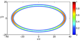
Figure 1: Result of the numerical integration of the 2D Schrödinger equation in the case of an elliptical waveguide with strong transverse confinement. Parameters: semiaxis $b/\sigma\simeq 34.5$; $a/\sigma\simeq 15.6$.

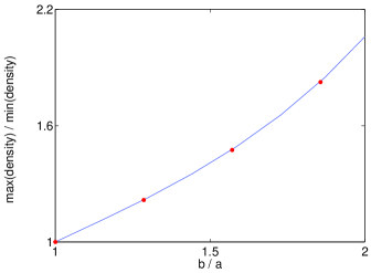
Figure 2: Result of the numerical integration of the Schrödinger equation in the case of an elliptical waveguide with strong transverse confinement. The graph shows the ratio between the density at the extrema of the two orthogonal axes of the ellipse, as a function of the ratio between the length of theses axes $b/a$. The points come from the simulation of the 2D Schrödinger equation in cartesian coordinates, while the full line comes from the 1D simulation of equation (24).

III.1 Effect of a longitudinal variation of $\omega_{\perp}$

The case of a transverse trapping frequency $\omega_{\perp}(s)$ with a non-trivial dependence on the longitudinal coordinate $s$ is addressed in the present section. This induces a longitudinal variation of the transverse wavefunction $f_{0s}$ and introduce new terms in $\hat{H}_{g}$ due to the non-vanishing longitudinal derivatives of $f_{0s}$. Applying the same procedure as in the previous section, and limiting ourselves to the first order in $\kappa^{2}\sigma^{2}$, we get the following 1D effective equation for $g(s)$

$$\mu\,g=-\frac{\hbar^{2}}{2M}\frac{\textrm{d}^{2}g}{\textrm{d}s^{2}}+\left[\hbar\omega_{\perp}+V_{\rm ext}-\frac{\hbar^{2}\kappa^{2}}{8M}+\frac{\hbar^{2}}{16M}\frac{\omega_{\perp}^{\prime 2}}{\omega_{\perp}^{2}}\right]\,g.$$ (28)

The dependence of $\omega_{\perp}$ on $s$ not only gives an $s$-dependent potential energy equal to zero-point energy $\hbar\omega_{\perp}(s)$, but also adds a further contribution proportional to $\omega_{\perp}^{\prime 2}/\omega_{\perp}^{2}$. Consistency with our decoupling procedure requires that $|\omega_{\perp}^{\prime}|\lessapprox\kappa\,\omega_{\perp}$ and $|\omega^{\prime\prime}_{\perp}|\lessapprox\kappa^{2}\omega_{\perp}$. This implies in particular that the term proportional to $\omega_{\perp}^{\prime 2}/\omega_{\perp}^{2}$ is much smaller than the zero-point energy term.

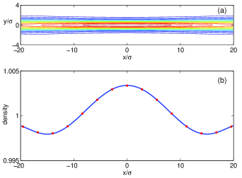
Figure 3: (a) Result of the numerical integration of the 2D Schrödinger equation in the case of an straight waveguide with a strong confinement of spatially-dependent transverse confinement frequency $\omega_{\perp}(x)=\omega_{\perp}\sqrt{1+4(\delta\omega_{\perp}/\omega_{\perp})\,\cos(\pi x/\lambda)}$. The colour code is the same as in Fig.1. Parameters: $\delta\omega_{\perp}/\omega_{\perp}=0.1$, $\lambda/\sigma\simeq 22.4$. An external potential such that $V_{\rm ext}+V_{\perp}=M\omega_{\perp}(x)^{2}y^{2}/2-\hbar\omega_{\perp}(x)/2$ has been introduced in order to compensate the spatial modulation of the zero-point trapping energy. (b) comparison between the 2D density integrated along direction y (red dots) and the solution if the effective 1D Schrödinger equation (full line).

In order to check the effect of the new potential term proportional to $\omega_{\perp}^{\prime 2}/\omega_{\perp}^{2}$, we have numerically solved the 2D Schrödinger equation in cartesian coordinates for the case of a straight waveguide with a modulated $\omega_{\perp}(s)$. In order to put the effect of the $\omega_{\perp}^{\prime 2}/\omega_{\perp}^{2}$ in better evidence, the external potential $V_{\rm ext}$ has been chosen in such a way to compensate the modulation of the zero-point energy of the transverse harmonic trapping $\hbar\omega_{\perp}(s)/2+V_{\rm ext}(s)=0$. As shown in Fig.3, the density modulation has indeed the same periodicity of $\omega_{\perp}^{\prime 2}/\omega_{\perp}^{2}$ and is in quantitatively good agreement with the numerical solution of the one-dimensional equation (28).

III.2 Effect of interatomic interactions

In a 3D geometry, mean-field interactions are included in the the Gross-Pitaevskii equation book as nonlinear terms of the form:

$$V_{int}=g_{3D}N_{0}\left|\frac{f_{s}(u,v)g(s)}{\sqrt{h(s,u,v)}}\right|^{2}\;,$$ (29)

being $g_{3D}=4\pi\hbar^{2}a_{3D}/M$, $a_{3D}$ the three-dimensional scattering length and $N_{0}$ is the total number of atoms notation . The Gross-Pitaevskii equation in presence of a periodic potential has been extensively studied in the context of Bose-Einstein condensates in optical lattices. The issue of the factorization of the wavefunction in its transverse and longitudinal part in the presence of interactions is in general a non trivial one.

In the language of the present paper, the presence of interactions requires that the transverse wavefunction $f_{0}(u,v)$ is now solution of the ground state Gross-Pitaevskii equation

$$\Big{[}-\frac{\hbar^{2}}{2m}(\partial^{2}_{uu}+\partial^{2}_{vv})+N_{0}\,g_{3D}\,|g(s)|^{2}\,|f_{0s}(u,v)|^{2}+\\ +V_{\perp}(u,v)\Big{]}f_{0s}(u,v)=\mu_{\perp}\,f_{0s}(u,v)$$ (30)

which results from the inclusion of the mean-field interaction term into the transverse Hamiltonian (20). Here $\mu_{\perp}$ has the meaning of a transverse chemical potential. In the general case, Eq. (30) has to be solved self-consistently with the equation determining the longitudinal wavefunction $g(s)$, which can be a computationally intensive task unless clever schemes are adopted, as e.g. in NPGPE .

A very simple formulation can be obtained in the limiting case of very strong radial confinement, when interactions have a negligible effect on the shape of the transverse ground state wavefunction $f_{0}(u,v)$. In this limit, interactions only provide a mean-field energy term proportional to the local density to be included in the longitudinal equation. This has then the usual form of a 1D Gross-Pitaevskii equation including the curvature term discussed in the previous section

$$(\mu-\hbar\omega_{\perp})g(s)=-\frac{\hbar^{2}}{2M}\frac{\textrm{d}^{2}g(s)}{\textrm{d}s^{2}}+V_{\rm ext}(s)g(s)\\ -\frac{\hbar^{2}\kappa^{2}(s)}{8M}g(s)+g_{1D}N_{0}|g(s)|^{2}g(s),$$ (31)

where the effective 1D coupling constant is defined as:

$$g_{\textrm{1D}}=\frac{4a_{3D}\hbar^{2}}{M\sigma^{2}}\;.$$ (32)

IV Case of a rotating waveguide

We now turn to the more general case of a rotating waveguide. For simplicity, we shall from now on assume that the curve $\mathcal{C}$ is included in the plane $(x,y)$, that the rotation vector $\mathbf{\Omega}$ is orthogonal to this plane, and that the origin of $\mathbf{r}_{\mathcal{C}}$ coincides with the centre of rotation. We shall furthermore consider in what follows the case of a constant $\omega_{\perp}$ independent of the position on the curve.

Repeating the same steps as in Sec. III, the transverse Hamiltonian can be decomposed as

$$\hat{h}=\tilde{H}_{0}+\tilde{W}\;,$$ (33)

with

$$\tilde{H}_{0}=\frac{\hbar^{2}g}{2M}\left(i\partial_{u}-\frac{M\Omega r_{t}}{\hbar}\right)^{2}-\frac{\hbar^{2}g}{2M}\partial^{2}_{vv}+gV_{\perp}\;,$$ (34)

and

$$\tilde{W}=W+i\hbar\Omega\bigg{[}\frac{gr_{t}\kappa}{2h}+\frac{u}{h}g^{\prime}-\frac{guh^{\prime}}{2h^{2}}+r_{n}g^{\prime}\\ -\frac{gr_{n}h^{\prime}}{2h^{2}}+\frac{gu}{h}\partial_{s}+\frac{gr_{t}}{h}\partial_{s}\bigg{]}-\frac{1}{2}M\Omega^{2}r_{t}^{2}g\;.$$ (35)

In the last expression, the following shorthand notations have been used: $r_{t}=\mathbf{r}_{\mathcal{C}}\cdot\mathbf{t}$ and $r_{n}=\mathbf{r}_{\mathcal{C}}\cdot\mathbf{n}$. The ground state of $\tilde{H}_{0}$ is now given by

$$\tilde{f}_{0s}(u,v)=f_{0}(u,v)\,e^{-iM\Omega r_{t}u/\hbar}\;.$$ (36)

Assuming a moderate rotation speed $|\Omega|\ll\omega_{\perp}$ and $M\Omega^{2}\mathbf{r}_{\mathcal{C}}^{2}\ll\hbar\omega_{\perp}$, an explicit calculation of the longitudinal derivatives of $\tilde{f}_{0s}$ shows that the following inequalities are satisfied

$$\left|\frac{\partial\tilde{f}_{0s}}{\partial s}\right|\ll\left|\frac{\tilde{f}_{0s}}{\sigma}\right|\qquad\textrm{and}\qquad\left|\frac{\partial^{2}\tilde{f}_{0s}}{\partial s^{2}}\right|\ll\left|\frac{\tilde{f}_{0s}}{\sigma^{2}}\right|,$$ (37)

which guarantee that $\tilde{W}$ can be treated as a small perturbation with respect to $\tilde{H}_{0}$. To the first order in $\kappa^{2}\sigma^{2}$, one then has

$$\hat{H}_{g}g(s)=\int\!\int\!\textrm{d}u\,\textrm{d}v\,\tilde{f}_{0s}^{*}(\tilde{H}_{0}+\tilde{W})\tilde{f}_{0s}=\\ =-\frac{\hbar^{2}}{2M}g^{\prime\prime}+\left[\hbar\omega_{\perp}+V_{\rm ext}-\frac{\hbar^{2}\kappa^{2}}{8M}-\frac{M\Omega^{2}}{2}r_{t}^{2}\right]\,g\\ +i\hbar\Omega\left[\frac{r_{t}\kappa}{2}\,g+r_{n}\,g^{\prime}\right]$$ (38)

and the 1D equation for the rotating waveguide can finally be written as

$$\mu\,g=\frac{1}{2M}\left[i\hbar\frac{\textrm{d}}{\textrm{d}s}+M\,\mathbf{t}\cdot\left(\mathbf{r}_{C}\times\mathbf{\Omega}\right)\right]^{2}g\\ +\left[\hbar\omega_{\perp}+V_{\rm ext}-\frac{\hbar^{2}\kappa^{2}}{8M}-\frac{1}{2}M\Omega^{2}\mathbf{r}_{C}^{2}\right]g\;,$$ (39)

where we have used the identity $\textrm{d}r_{n}/\textrm{d}s=\kappa r_{t}$. As compared to the non-rotating case of (24), additional terms appear here due to the rotation. The first one is the one-dimensional form of the gauge term appearing in the kinetic energy term in the rotating frame and mostly affects the phase of the wavefunction. The second rotation-induced term is the classical centrifugal energy term. This term, along with the curvature-induced term, the external potential term, and the zero-point energy term, can be used to transfer angular momentum from the trap to the atoms and then establish a finite phase circulation in the condensate.

IV.1 Analogy with optical lattices

Consider for simplicity a circular waveguide of radius $R$ in the presence of a rotating periodic potential of period $2\pi/\ell$ ($\ell$ is integer) in the angular coordinate $\theta$

$$V(\theta,t)=V_{0}\cos[\ell(\theta-\Omega t)].$$ (40)

Once mean-field interactions are included in the same way as done in (31), equation (39) can be casted in the simple form

$$\left[-\frac{\partial^{2}}{\partial\theta^{2}}+i\Omega\frac{\partial}{\partial\theta}+V_{0}\cos(\ell\theta)+{\tilde{g}}|\varphi|^{2}\right]\varphi(\theta)={\tilde{\mu}}\varphi(\theta)$$ (41)

which shows a strong formal analogy with the problem of a Bose-Einstein condensate in a 1D optical lattice with periodic boundary conditions  Ueda . Here, $\varphi(\theta)$ is the longitudinal wavefunction, $\tilde{g}$ is the coupling constant due to interatomic interactions, $\tilde{\mu}$ is the chemical potential shifted by constant potential terms and all energies have been expressed in units of $\hbar^{2}/(2MR^{2})$. The quantity $\Omega/2$ plays the role of the quasi-momentum for a Bloch wave in the periodic potential of the lattice, with a subtle difference arising from the different periodic boundary conditions: in the periodic potential of the lattice, the allowed values of quasi-momentum are integer multiples of $\hbar 2\pi/Nd$, $d$ being the lattice spacing and $N$ being the number of lattice wells present in the system. On the other hand, all values of $\Omega$ are allowed in the present case of a rotating waveguide, the single-valuedness of the wavefunction $\varphi(\theta)$ being ensured by the Bloch theorem on the whole length of the ring, i.e. $\varphi(\theta+2\pi/\ell)=\exp[i2n\pi/\ell]\varphi(\theta)$ with $n$ integer. The complete band structure is generated by the set of values $n=0,1,2,\dots\ell-1$, giving rise to $\ell$ independent sub-bands periodic in $\Omega$ with period $2\ell$.

The circulation of the different states is a function of $n$ and $\Omega$ (for instance the lowest energy states at $2n-1<\Omega<2n+1$ have circulation $n$). The $\ell$-fold modulation of the potential along the waveguide allows only mixing of states at circulation $n$ with states at circulation $n\pm\ell$, in correspondence of the sub-band gaps. Hence, following adiabatically a given sub-band by very slowly increasing (or decreasing) the rotation frequency, one can transform a state at a given circulation $n$ into a state at circulation $n\pm\ell$.

V Experimental issues

A possible way of achieving experimentally an annular condensate with strong transverse confinement is to use a magnetic toroidal trap, as reported in Stamper_Kurn ; Riis . In this section, a completely different experimental configuration is proposed, and its advantages pointed out. For the sake of simplicity, we shall concentrate our attention to the most relevant case of a planar waveguide whose axis lays on the horizontal $xy$ plane. A strong confinement in the vertical $z$ direction can be obtained using a horizontal light sheet which provides a potential $V_{z}(z)$, while the curvilinear waveguide profile can be created by rapidly moving the focus point of a red-detuned laser beam (acting as an optical tweezer tweezer ) along the curve $\mathcal{C}$, at a, possibly time-dependent speed $v(t)$. This can be obtained e.g. by reflecting the laser light onto vibrating mirrors or using acousto-optic modulators. If the movement of the focus point is much faster than the transverse trapping frequency, then the atoms will see the following averaged potential

$$V(x,y,z)=V_{z}(z)+\int_{0}^{T}\frac{\textrm{d}t}{T}V_{\textrm{tw}}(x-x_{\mathcal{C}}(t),y-y_{\mathcal{C}}(t)),$$ (42)

where $V_{z}(z)$ is the trapping potential due to the light sheet and $V_{\textrm{tw}}(x,y)$ the trapping potential due to the optical tweezer. The pair $(x_{\mathcal{C}}(t),y_{\mathcal{C}}(t))$ defines the position of the laser focus on the $xy$ plane at time $t$, which spans the curve ${\mathcal{C}}$ in the period $T$ ($x$ and $y$ are here cartesian coordinates). The tweezer potential is attractive, and can be taken as having a Gaussian shape of waist $w$ and peak value $V_{\rm tw}^{0}<0$

$$V_{\rm tw}(x,y)=V_{\rm tw}^{0}\,\exp[-(x^{2}+y^{2})/w^{2}].$$ (43)

It is then easy to obtain expressions for the potential terms $V_{\perp}$ and $V_{\rm ext}$ appearing in the Hamiltonian (12)

$$\omega_{\perp}^{2}(s) = \frac{\sqrt{\pi}w}{T\,v(s)}\,\omega_{\textrm{tw}}^{2}\quad\textrm{with}\quad\omega_{\textrm{tw}}^{2}=\frac{2|V_{\rm tw}^{0}(s)|}{mw^{2}}\,,$$ (44)

$$V_{\rm ext}(s) = \frac{\sqrt{\pi}w}{T\,v(s)}\,V_{\rm tw}^{0}(s).$$ (45)

A remarkable fact has to be noted: both $\omega_{\perp}^{2}(s)$ and $V_{\rm ext}(s)$ are inversely proportional to the speed of the laser focus when passing in the neighbourhood of the point $s$ under examination, and to its overall orbital period. A possible way of adding a spatially modulated external potential along the waveguide is therefore to simply modulate the speed of motion of the focus along the curve.

Plugging in (44) typical values of intensity $I=100$ W and detuning $\delta=300$ nm for optical tweezers with $w=30$ $\mu$m, one can see that transverse extensions as low as 1.16 $\mu$m could be achieved on a 150 $\mu$m radius torus with such a device, ensuring the validity of the strong confinement hypothesis. The main advantage of this method over the magnetic traps studied e.g. in Stamper_Kurn is that any shape of the curve $\mathcal{C}$ can be obtained without any additional difficulty, and this can also be modified in the course of the experiment in order to obtain e.g. a rotating waveguide.

Another important requirement for the study of supercurrent to be possible is that the longitudinal potentials are not strong enough to fragment the condensate. As an example, it is interesting to estimate the effect of a tilting of the light sheet that is used to vertically confine the atoms. For a tilting angle $\alpha$ from the horizontal, the potential energy difference at the extrema of the waveguide due to gravity is equal to $2Mg_{G}R\sin\alpha$, where $g_{G}$ is the gravity field acceleration and $2R$ is the horizontal distance between opposite points of the waveguide. Within the Thomas-Fermi approximation, fragmentation occurs if the gravitational energy difference is larger than the mean-field interaction energy, that is if

$$2Mg_{G}R\sin\alpha>\frac{g_{1D}N_{0}}{2\pi R}.$$ (46)

For a system of $N_{0}=10^{6}$ atoms of ⁸⁷Rb with scattering length $a=5.77$ nm in a waveguide of radius $R=150\,\mu$m and $\sigma=1.16\,\mu$m, the system remain connected provided $\alpha<0.15^{\circ}$, which is a rather stringent but not unreachable experimental requirement. Note that the gravitational potential does not rotate with the waveguide when this is set into rotation, so that it might possibly act as a defect moving through the one-dimensional fluid Pavloff ; Ueda2 .

In the case of very tight confinement and frozen transverse dynamics the issue of phase fluctuations in the 1D condensate comes into play. We believe that the rotational properties of the condensate should not however be disturbed at least in the meanfield regime at low enough temperature.

Another issue of great importance from the experimental point of view is the possibility of measuring the number of vorticity quanta present around the annular condensate. A measurement after expansion has been recently predicted to be able to provide a clear answer tozzo , but a non-destructive measurement would be preferable in view of applications as a rotation sensor. In the case of a rotating non-circular (e.g., elliptical) waveguide, the deformation of the periodic density modulation due to the centrifugal potential should in principle provide a way of measuring the supercurrent. If this signal is too weak to be detected, one could still resort to other techniques, e.g. the analysis of collective modes brian or the measurement of the momentum distribution by means of Bragg spectroscopy muniz06 or slow-light imaging slowlight .

VI Conclusion

In this paper, we have developed a formalism which is able to reduce the three-dimensional problem of atomic propagation along an atomic waveguide to one-dimensional equations. Under a strong transverse confinement hypothesis, the transverse extension of the wavefunction is much smaller than the curvature radius of the waveguide and the wavefunction can be factorized into the product of its longitudinal and transverse parts. Our formalism is then applied to a novel concept of optical waveguide which combines the possibility of having a strong confinement with a great flexibility in the design of the, possibly rotating, waveguide shape.

Such a description provides a simple yet accurate starting point for analytical studies and numerical simulations, as well as for the design of experimental setups. Our framework is in fact able to considerably simplify the theoretical analysis while still keeping track of the relevant degrees of freedom in a quantitative way. Possible applications range from the determination of the best experimental sequence to nucleate a supercurrent along a ring-shaped Bose-Einstein condensate, to the study of the response to a global rotation in a sort of matter-wave gyroscope.

- (1) A. Leggett, Rev. Mod. Phys. 73, 307 (2001).
- (2) T. L. Gustavson et al., Phys. Rev. Lett. 78, 2046 (1997).
- (3) W. Macek and D. Davis, Applied Phys. Lett. 2, No. 3, 67 (1963).
- (4) F. Bloch, Phys. Rev. A 7, 2187 (1973).
- (5) H. Saito and M. Ueda, Phys. Rev. Lett. 93, 220402 (2004).
- (6) K. Kasamatsu, M. Tsubota and M. Ueda, Phys. Rev. A 66, 053606 (2002).
- (7) P. Leboeuf and N. Pavloff, Phys. Rev. A 64, 033602 (2001).
- (8) L.P. Pitaevskii and S. Stringari, Bose-Einstein Condensation , Clarendon Press Oxford (2003).
- (9) The coupling constant should not be confused with the longitudinal wavefunction .
- (10) E. J. Mueller, Phys. Rev. A 66, 063603 (2002).
- (11) M. Machholm, C. J. Pethick, and H. Smith, Phys. Rev. A 67, 053613 (2003).
- (12) B. Wu and Q. Niu, Phys. Rev. A 64, 061603 (2001).
- (13) C. Menotti, A. Smerzi and A. Trombettoni, New Journal of Physics 5, 112 (2003).
- (14) Gh.-S. Paraoanu, Phys. Rev. A 67, 023607 (2003).
- (15) L. Fallani, L. De Sarlo, J. E. Lye, M. Modugno, R. Saers, C. Fort, and M. Inguscio, Phys. Rev. Lett. 93, 140406 (2004).
- (16) B. Eiermann, Th. Anker, M. Albiez, M. Taglieber, P. Treutlein, K.-P. Marzlin, and M. K. Oberthaler, Phys. Rev. Lett. 92, 230401 (2004).
- (17) Trapping of neutral atoms and molecules in toroidal storage rings were also recently reported in e.g. J. A. Sauer, M. D. Barrett, and M. S. Chapman, Phys. Rev. Lett. 87, 270401 (2001), F. M. H. Crompvoets et al., Nature (London) 411, 174 (2001).
- (18) S. Gupta, K. W. Murch, K. L. Moore, T. P. Purdy and D. M. Stamper-Kurn, Phys. Rev. Lett. 95, 143201 (2005).
- (19) A. S. Arnold, C. S. Garvie, and E. Riis, Phys. Rev. A 73, 041606 (2006)
- (20) S. Chu et al., Phys. Rev. Lett. 57, 314 (1986).
- (21) A. S. Arnold, J. Phys. B: At. Mol. Opt. Phys. 37, L29 (2004); M. B. Crookston, P. M. Baker, and M. P. Robinson, J. Phys. B: At. Mol. Opt. Phys. 38, 3289 (2005); W. Rooijakkers, Appl. Phys. B 78, 719 (2004); O. Morizot, Y. Colombe, V. Lorent, H. Perrin, B. M. Garraway, preprint physics/0512015.
- (22) M. P. Do Carmo, Differential geometry of curves and surfaces (Prentice Hall, Englewood Cliffs, 1976).
- (23) C. Cohen-Tannoudji, B. Diu, F. Laloë, Quantum mechanics (Wiley-Interscience, 1977)
- (24) L. Salasnich, A. Parola, and L. Reatto, Phys. Rev. A 65, 043614 (2002).
- (25) L. D. Landau and E. M. Lifshitz, Statistical Mechanics, Addison-Wesley, Reading, MA (1969).
- (26) C. Cohen-Tannoudji, lecture notes at Collège de France, academic year 2001-2002, available at the website: http://www.phys.ens.fr/cours/college-de-france/2001-02/2001-02.htm.
- (27) M. Modugno, C. Tozzo, and F. Dalfovo, preprint cond-mat/0605183.
- (28) M. Cozzini, B. Jackson, and S. Stringari, Phys. Rev. A 73, 013603 (2006).
- (29) S. R. Muniz, D. S. Naik, and C. Raman, Phys. Rev. A 73, 041605(R) (2006).
- (30) M. Artoni and I. Carusotto, Phys. Rev. A 67, 011602 (2003).