Quantum limits to center-of-mass measurements

Abstract

We discuss the issue of measuring the mean position (center-of-mass) of a group of bosonic or fermionic quantum particles, including particle number fluctuations. We introduce a standard quantum limit for these measurements at ultra-low temperatures, and discuss this limit in the context of both photons and ultra-cold atoms. In the case of fermions, we present evidence that the Pauli exclusion principle has a strongly beneficial effect, giving rise to a $1/N$ scaling in the position standard-deviation – as opposed to a $1/\sqrt{N}$ scaling for bosons. The difference between the actual mean-position fluctuation and this limit is evidence for quantum wave-packet spreading in the center-of-mass. This macroscopic quantum effect cannot be readily observed for non-interacting particles, due to classical pulse broadening. For this reason, we also study the evolution of photonic and matter-wave solitons, where classical dispersion is suppressed. In the photonic case, we show that the intrinsic quantum diffusion of the mean position can contribute significantly to uncertainties in soliton pulse arrival times. We also discuss ways in which the relatively long lifetimes of attractive bosons in matter-wave solitons may be used to demonstrate quantum interference between massive objects composed of thousands of particles.

I Introduction

The topic of mesoscopic quantum effects is of great current interest, especially in photonic or in ultra-cold atomic systems where a large decoupling from the environment is possible. An important degree of freedom is the average or center-of-mass position of a large number of particles. It is now possible to observe quantum diffraction of the center-of-mass in molecules like C₆₀ and related fullerenesZeil . Larger physical systems would provide an even a stronger test of quantum theoretical predictions. As well as testing quantum theory in new, mesoscopic regimes, these types of experiment have potential applications to novel sensors. For example, ultra-precise measurements of position may be useful in measuring gravitational interactions, or other forces that couple to conserved quantities.

In this paper, we wish to examine the quantum limits to center-of-mass position fluctuations. We further discuss these limits in the context of mesoscopic systems of interacting particles, atoms or molecules. This is an important issue in quantum-optical or ultra-cold atom environments, where center-of-mass motion places a limit on coherence properties of photonic or atom lasers. A localized system of particles features a dual particle and wave nature, that is, it has conjugate observables of momentum and position, as well as conjugate observables of number and phase. As pointed out by Landau and PeierlsLandau , free particle momentum is a QND observable. In fact, the momentum of a quantum soliton can be non-destructively measured via the position of a probe soliton after their collisionWatanabe . The quantum position fluctuation increases with propagation distance due to an initial momentum uncertainty. This places a fundamental limit on momentum QND measurements.

We generalize the concept of the standard quantum limit of a mean position measurement Lai ; FiniHagelstein to any kind of quantum field. The standard quantum limit is defined here as the position uncertainty of a many-body ground-state for non-interacting particles with a given density distribution and total momentum. For massive particles, this corresponds to the Heisenberg-limited uncertainty of the center-of-mass of a group of non-interacting particles in an external potential, at zero temperature. Intriguingly, we find completely different scaling laws for different particle statistics: while bosons have a position uncertainty (standard deviation) that scales as $1/\sqrt{N}$, fermionic center-of-mass uncertainties scale as $1/N$ for $N$ particles. This is caused by the particle correlations induced by Fermi statistics. The scaling indicates that ultra-cold fermions are the preferred system for ultra-sensitive measurements of center-of mass.

A necessary requirement for quantum-limited measurements is an extremely low level of fluctuations and noise, which makes laser pulses and ultra-cold atoms the most reasonable choices at present. As an example, the localized solitons of the attractive one-dimensional Bose gas can now be observed both in quantum-optical and in atom-optical environments. As well as technological applications in communications, these types of soliton show intrinsic quantum effects. That is, the effects of quantum phase diffusion (squeezing)Carter ; Lai ; DrCorney have been observed in experimentsRosenbluh ; Nature ; CorneyLeuchs . Quantum correlations established by soliton collision (quantum non-demolition measurement)Watanabe have also been demonstrated in experimentFriberg . Even though they involve up to $10^{9}$ particles, these effects simply do not occur in classical soliton theory.

Phase squeezing or phase QND measurement does not lead to center-of-mass changes, which are especially interesting for massive particles, as this degree of freedom is coupled directly to the gravity field. Due to problems in quantizing gravity, there have been suggestions that gravitational effects may lead to wave-packet collapse and/or dissipationDiosi ; Ghirardi ; Penrose ; Tod ; Filippo . While this remains speculative, it is clearly an area of quantum mechanics where there are no existing tests. To exclude such theories, one would need to violate a classical inequality involving mesoscopic numbers of massive particles, whose center-of-mass was in some type of quantum superposition stateReidCaval . In real experiments, weak localizationAharonov can take place due to interactions with the environment. It is at least interesting to investigate how this may occur, as a first step towards testing more fundamental types of localization. We note that steps in this direction have been taken recently for non-interacting, massless particles, via position observations with photons, at the standard quantum limit or betterTrepsetal ; Kolobov .

Quantum wave-packet spreading of the center-of-mass is an intrinsic quantum prediction for untrapped particles at all particle numbers. However, this is masked by the single-particle effects analogous to classical pulse broadening for an optical pulse in a linear dispersive medium. A soliton or quantum bound-state can suppress this single-particle or classical pulse broadening, and allows the intrinsic center-of-mass quantum spreading to be observed FiniHagelstein , in a similar way to the known quantum noise effects found in amplified solitonsGordon . We find that this is an exactly soluble problem for any initial quantum state. No linearization or decorrelation approximation is needed, which allows us to examine quantum wave-packet spreading over arbitrary distance scales. In order to distinguish classical pulse broadening from quantum wave-packet spreading, we calculate the standard quantum limit of this measurement for an initially coherent soliton pulse. This requires knowledge of the time-evolution of the density distribution for an interacting many-body system, which is nontrivial, and requires numerical solutions.

II Center of mass operators

We start by noting that while a centroid exists for any localized, measurable quantity, it is most interesting for a conserved quantity. For any physical system with a conserved current four-density $\widehat{j}=\left(j_{0,}\mathbf{j}\right)$, it is possible to define a center-of-charge (or mass, energy, etc) relative to the conserved quantities

$$\widehat{J}_{\mu}=\int\hat{j}_{\mu}\left(\mathbf{x}\right)d^{D}\mathbf{x}\,\,.$$ (1)

In a quantum state that is an eigenstate of the conserved charge with $J_{0}>0$, defined on a $D$- dimensional space, the definition of the centroid is:

$$\hat{\mathbf{x}}_{J}=\frac{1}{J_{0}}\int\mathbf{x}\hat{j}_{0}\left(\mathbf{x}\right)d^{D}\mathbf{x}\,\,.$$ (2)

After partial integration, the conservation law,

$$\frac{\partial\widehat{j}_{0}}{\partial t}+\nabla\cdot\hat{\mathbf{j}}=0\,\,,$$ (3)

then implies that the centroid position translates with a velocity given by the spatial part of the conserved current:

$$\frac{\partial\hat{\mathbf{x}}_{J}}{\partial t}=\frac{\hat{\mathbf{J}}}{J_{0}}\,\,.$$ (4)

While the concept of measuring the center of mass position is well-known, there are a number of issues involved. The most obvious is that there is a difference between the center-of-mass and the average position of a group of non-identical particles. This difference vanishes for non-relativistic particles all of the same mass: for example, isotopically pure, ultra-cold atoms. However, there is a real difference in the case of particles of different masses, and for extremely relativistic particles and photons, where the effective mass depends on the momentum. Here the average position differs from the center-of-mass. Another subtlety which this paper treats in some detail, occurs when the system is in a quantum mixture of different particle numbers: the effects of this are treated in the remainder of this section.

II.1 Massive fields

We first consider non-relativistic massive quantum fields $\hat{\Psi}_{i}\left(\mathbf{x}\right)$, where each component has an equal mass. The fundamental particle statistics can be either fermionic or bosonic. As usual for quantum fields, the commutators are:

$$\left[\hat{\Psi_{i}}\left(t,\mathbf{x}\right),\hat{\Psi}_{j}^{\dagger}\left(t,\mathbf{x}^{\prime}\right)\right]_{\pm}=\delta_{ij}\delta^{3}\left(\mathbf{x}-\mathbf{x}^{\prime}\right).$$ (5)

Introducing the particle density

$$\hat{n}\left(\mathbf{x}\right)=\sum_{i}\hat{n}_{i}\left(\mathbf{x}\right)=\sum_{i}\Psi_{i}^{\dagger}\left(\mathbf{x}\right)\hat{\Psi}_{i}\left(\mathbf{x}\right),$$ (6)

we can define the total particle number

$$\hat{N}=\int d^{D}\mathbf{x}\hat{n}\left(\mathbf{x}\right),$$ (7)

which is exactly conserved in the absence of dissipative processes like absorption or amplification. In this paper, we will consider cases where the system has an uncertainty in $\hat{N}$, but we will exclude states with zero particle number. In terms of operational measurements with small particle numbers, this may require post-selection to exclude states of this type - since of course the center-of-mass is undefined in such cases.

In order to define center-of-mass or mean position for systems with particle number fluctuations, several definitions are possible, depending on measurement procedures. There is more than one measurement procedure possible, since the quantum state need not be an eigenstate of the number operator. Hence, different number states could have an arbitrary relative weighting.

In the absence of external potentials, systems of interacting particles also have an invariant quantity due to translational invariance, which is the total momentum (in $D$ dimensions):

$$\hat{\mathbf{P}}=\frac{\hbar}{2i}\int\left[\hat{\Psi}_{i}^{\dagger}\left(\mathbf{x}\right)\mathbf{\nabla}\hat{\Psi}_{i}\left(\mathbf{x}\right)-\nabla\hat{\Psi}_{i}^{\dagger}\left(\mathbf{x}\right)\hat{\Psi}_{i}\left(\mathbf{x}\right)\right]d^{D}\mathbf{x}$$ (8)

Here we use the Einstein summation convention for repeated indices. We use a capital letter to emphasize that this is an extensive quantity, proportional to the number of particles.

II.2 Massless fields

Massless fields - photons - are the most commonly used particles where measurements are made at the quantum level. In this case, we can distinguish two different important cases.

• Narrow band fields in one-dimensional wave-guides or fibers experience dispersion, which causes them to behave as massive particles. In a similar way, the paraxial approximation for beams allows diffractive behavior to be treated in an effective mass approximation. These cases can be handled in the same way as the treatment given above.

• More fundamental issues arise in free-space, where there is a long-standing fundamental problem of how to define photon position. In addition, as there is no photon mass, even the idea of center-of-mass requires care. Instead, one must either use the concept of a center-of-energy, or of a center of photon-number. We shall focus on the latter concept here.

To treat the free-space average position, we can use a conserved local density obtained from the dual symmetry properties of Maxwell equationsDual . We introduce $\hat{\mathbf{\mathcal{E}}}_{\sigma}$, where $\sigma=\pm 1$, which are the helicity components of the complex Maxwell fields in units where $c=\varepsilon_{0}=\mu_{0}=1$, and the corresponding complex vector potentials $\hat{\mathbf{\mathcal{A}}}_{\sigma}$ , so that:

$$\hat{\mathbf{\mathcal{E}}} = \hat{\mathbf{E}}+i\hat{\mathbf{B}}$$

$$= \nabla\times\hat{\mathbf{\mathcal{A}}}$$

$$= \hat{\mathbf{\mathcal{E}}}_{+}+\hat{\mathbf{\mathcal{E}}}_{-}\,\,.$$

It is easily checked from the complex form of Maxwell’s equations that $i\partial\hat{\mathbf{\mathcal{E}}}_{\sigma}/\partial t=\nabla\times\hat{\mathbf{\mathcal{E}}}_{\sigma}$and $i\partial\hat{\mathbf{\mathcal{A}}}_{\sigma}/\partial t=\nabla\times\hat{\mathbf{\mathcal{A}}}_{\sigma}$. The photon density is then:

$$\hat{n}\left(\mathbf{x}\right)=\sum_{\sigma}\hat{n}_{\sigma}\left(\mathbf{x}\right)=\frac{\sigma}{4}:\left(\hat{\mathbf{\mathcal{E}}}_{\sigma}^{\dagger}\cdot\hat{\mathbf{\mathcal{A}}}_{\sigma}+\hat{\mathbf{\mathcal{E}}}_{\sigma}\cdot\hat{\mathbf{\mathcal{A}}}_{\sigma}^{\dagger}\right):\,\,,$$ (9)

with a corresponding conserved current of :

$$\widehat{\bm{J}}=\sum_{\sigma}\frac{\sigma}{4i}:\left(\hat{\mathbf{\mathcal{E}}}_{\sigma}^{\dagger}\times\hat{\mathbf{\mathcal{A}}}_{\sigma}+\hat{\mathbf{\mathcal{A}}}_{\sigma}^{\dagger}\times\hat{\mathbf{\mathcal{E}}}_{\sigma}\right)\,\,.$$ (10)

We note that with these definitions, the photon density is not positive definite in small volumes and time-intervals. However, the total photon number $\widehat{N}$ is well-defined and positive definite, so that a position centroid is well-defined for this conserved quantity. For the remainder of this paper we will focus on non-relativistic massive particles for definiteness, while noting that many results that only depend on the existence of a conserved current will hold in the general case of a photon field.

II.3 Intensive position

For quantum states that are eigenstates of number with $N>0$, the obvious definition is:

$$\hat{\mathbf{x}}^{(N)}=\frac{\int\mathbf{x}\hat{n}\left(\mathbf{x}\right)d^{D}\mathbf{x}}{N}$$ (11)

This is undefined for the vacuum state, but is well-defined for all other number eigenstates. For the non-relativistic massive particle case, this obeys the expected commutation relation with the total momentum operator:

$$\left[\hat{x}_{i}^{(N)},\hat{P}_{j}\right]_{\pm}=i{\hbar\delta}_{ij}.$$

The presence of the vacuum in states composed of mixtures or superpositions of number eigenstates introduces the requirement of deciding which relative weights to use for different particle numbers. The important fact to note is that the mean position of any vacuum component is undefined and, as such, its presence does not contribute to one’s knowledge of the mean position. Accordingly, as mentioned previously, we choose to work in a restricted Hilbert space which does not include the vacuum state. Practically, this is equivalent to performing heralded particle number measurements where any null results are discarded. From a mathematical perspective, we work with a projected density operator $\rho^{\prime}=\hat{\mathcal{P}}\rho\hat{\mathcal{P}}$, where $\hat{\mathcal{P}}=(\hat{I}-|0\rangle\langle 0|)$. In order to extract position information from linear superpositions or mixtures of number states, we introduce the center-of-mass position operator which is well defined in our projected Hilbert space:

$$\hat{\mathbf{x}}=\frac{\int\mathbf{x}\hat{n}\left(\mathbf{x}\right)d^{D}\mathbf{x}}{\hat{N}}$$ (12)

This intensive quantity also obeys the expected commutation relation with $\hat{\mathbf{P}}$:

$$\left[\hat{x}_{i},\hat{P}_{j}\right]_{\pm}=i\hbar\delta_{ij}$$ (13)

Thus, provided any measurement of the vacuum is discarded, $\hat{\mathbf{x}}$ and $\hat{\mathbf{P}}$ form a pair of canonical conjugate variables with the dimensionless uncertainty relation

$$\langle\Delta\hat{x}_{i}^{2}\rangle\langle\Delta\hat{P}_{i}^{2}\rangle\geq\frac{\hbar^{2}}{4}$$ (14)

for states projected into our restricted Hilbert space.

II.4 Extensive position

Although $\hat{\mathbf{x}}$ has the usual definition of the mean position, it’s operational denominator makes it is difficult to measure using many standard techniques, or even to represent in a normally ordered form. We can also introduce an extensive position operator, which produces a result proportional to the number of particles as well as their position. We define:

$$\hat{\mathbf{X}}=\hat{\mathbf{x}}\hat{N},$$ (15)

which is well-defined without projection in the Hilbert space. However, $\hat{\mathbf{X}}$ and $\hat{\mathbf{P}}$ do not form a pair of canonical conjugate variables, since

$$[\hat{X}_{i},\hat{P}_{j}]_{\pm}=i\hbar\delta_{ij}\hat{N}.$$ (16)

Through the uncertainty relation, we see that $\hat{\mathbf{X}}$ is sensitive not only to positional fluctuations but also fluctuations in the total particle number or beam intensity:

$$\langle\Delta\hat{X}_{i}^{2}\rangle\langle\Delta\hat{P}_{i}^{2}\rangle\geq\frac{\hbar^{2}\langle\hat{N}^{2}\rangle}{4}.$$ (17)

Furthermore, as an extensive operator, $\hat{\mathbf{X}}$ transforms in the following way. In a new reference frame $S^{\prime}$ where $\mathbf{x}^{\prime}=\mathbf{x}+\Delta\mathbf{x}$, we find that

$$\hat{\mathbf{X}}^{\prime}=\hat{\mathbf{X}}+\Delta\mathbf{x}\hat{N}$$ (18)

rather than just being translated by a c-number.

We note that the extensive position does have a canonical conjugate partner, in terms of the intensive or mean momentum operator:

$$\hat{\mathbf{p}}=\frac{\hat{\mathbf{P}}}{\hat{N}}$$ (19)

with a corresponding commutator of:

$$[\hat{X}_{i},\hat{p}_{j}]_{\pm}=i\hbar\delta_{ij}$$ (20)

II.5 Quasi-intensive position operator

We will finally define a quasi-intensive position operator, which corresponds to the typical direct measurement procedures in optics. With this operator, the position is first measured with techniques that are extensive - but the final result is normalized by the average particle number. This has the property that in an ensemble with variable numbers of particles, more weight is given to those measurements that involve the most particles. Here:

$$\hat{\mathbf{\mathfrak{X}}}=\frac{\hat{\mathbf{X}}}{\langle\hat{N}\rangle}$$ (21)

which can still be considered a useful measure of the mean position of a particle distribution, especially in the limit of large $\langle\hat{N}\rangle$ where total number fluctuations are suppressed. Indeed, this is the variable that corresponds most closely to some earlier proposed operational measures of pulse position, measured using local oscillator or homodyne techniques. It is interesting to note that the conjugate variable, the mean momentum, is the same as for an extensive position. This is analogous to the mean frequency of a laser pulse in a dispersive medium, which also corresponds closely to standard operational measurements used in laser physics.

In order to measure fluctuations about $\langle\hat{\mathbf{X}}\rangle$ or $\langle\hat{\mathbf{\mathfrak{X}}}\rangle$, however, care must be taken due to the fact that $\hat{\mathbf{\mathfrak{X}}}$ transforms in the following way under translation:

$$\hat{\mathbf{\mathfrak{X}}}^{\prime}=\hat{\mathbf{\mathfrak{X}}}+\Delta\mathbf{x}\frac{\hat{N}}{\langle\hat{N}\rangle}.$$ (22)

By considering fluctuations about $\mathbf{x}^{\prime}=0$ in a new reference frame where $\mathbf{x}^{\prime}=\mathbf{x}-\langle\mathbf{\mathfrak{X}}\rangle$, we define

$$\Delta\hat{\mathbf{\mathfrak{X}}}=\hat{\mathbf{\mathfrak{X}}}-\langle\hat{\mathbf{\mathfrak{X}}}\rangle\frac{\hat{N}}{\langle\hat{N}\rangle}$$ (23)

and thus minimize the number fluctuation contribution. Following from Eq. 17, this obeys the uncertainty relation

$$\langle\Delta\hat{\mathbf{\mathfrak{X}}}_{i}^{2}\rangle\langle\Delta\hat{\mathbf{P}}_{i}\rangle\geq\frac{\hbar^{2}\langle\hat{N}^{2}\rangle}{4\langle\hat{N}\rangle^{2}}$$

as the total number and momentum operators commute.

In order to avoid complications arising from this issue, we will only consider isolated systems where it is always possible to find an inertial reference frame in which $\langle\hat{\mathbf{\mathfrak{X}}}\rangle=\langle\hat{\mathbf{P}}\rangle=0$.

III Quantum limits on position uncertainties

Intrinsic quantum uncertainty in the results of projective measurements is perhaps the most striking difference between quantum mechanical observables and classical variables. Here we seek to characterize this uncertainty in the center-of-mass (COM) measurement by introducing a standard quantum limit to the variance in the distribution of results. This is not a lower bound - there is none - but rather a natural limit that one can expect to achieve using standard cooling and/or stabilization methods. The question of exactly which state to use to calculate such a characteristic COM is difficult to answer uniformly, especially as the states accessible to bosonic systems are different to those accessible to fermionic systems.

For a system with known density distribution and exchange statistics, we define the standard quantum limit to the COM uncertainty to be the variance remaining when a non-interacting system of the same particles is reduced to zero temperature in an external potential that reproduces the given density distribution. It is important to note that this definition makes no restriction on the statistics of the characteristic system. However, we will find that the statistics do have a large effect on the way that the quantum limit scales for a given density.

In the following analysis, we consider the variance in the intensive mean position operator, in the form:

$$|\Delta\hat{\mathbf{x}}|^{2}=\frac{1}{\hat{N}^{2}}\int d^{D}\mathbf{x}d^{D}\mathbf{y}\left\{\Delta\mathbf{x}\cdot\Delta\mathbf{y}\hat{n}(\mathbf{x})\hat{n}(\mathbf{y})\right\}\,\,.$$ (24)

Re-arranging this expression by using normal-ordering and commutators gives the result that:

$$\left|\Delta\hat{\mathbf{x}}\right|^{2} = \frac{1}{\hat{N}^{2}}\left(\hat{N}\hat{\sigma}^{2}+:|\Delta\hat{\mathbf{X}}|^{2}:\right)$$ (25)

where we define the wavepacket variance operator

$$\hat{\sigma}^{2}=\frac{1}{\hat{N}}\int d^{D}\mathbf{x}\left\{\left|\Delta\mathbf{x}\right|^{2}\hat{n}(\mathbf{x})\right\}$$ (26)

and the normally ordered COM variance

$$:|\Delta\hat{\mathbf{X}}|: = \int d^{D}\mathbf{x}d^{D}\mathbf{y}\Delta\mathbf{x}\cdot\Delta\mathbf{y}$$ (27)

$$\times\sum_{ij}\hat{\Psi}_{i}^{\dagger}(\mathbf{y})\hat{\Psi}_{j}^{\dagger}(\mathbf{x})\hat{\Psi}_{j}(\mathbf{x})\hat{\Psi}_{i}(\mathbf{y}).$$

Note that the exact operator ordering in the last expression is important if the decomposition is to be correct for both Fermi and Bose field operators.

III.1 Bosonic fields

The simplest configuration for a system of degenerate bosons has all particles described by a single normalized mode function $\chi(\mathbf{x})$. Thus, the characteristic states considered here are formed using functions of the creation operator $\widehat{a}_{\chi}^{\dagger}=\int d^{D}\mathbf{x}\left\{\chi\left(\mathbf{x}\right)\hat{\Psi}^{\dagger}\left(\mathbf{x}\right)\right\}$.

III.1.1 Number states

Zero temperature bosonic number states can expressed in the following way:

$$\left|N\right\rangle=\frac{1}{\sqrt{N}}(\hat{a}^{\dagger})^{N}\left|0\right\rangle.$$ (28)

Evaluating the COM variance of this state using the above decomposition is straightforward as the expectation value of the normally ordered term $:|\Delta\hat{\mathbf{x}}|^{2}:$ vanishes, leaving

$$\langle|\Delta\hat{\mathbf{x}}|^{2}\rangle=\frac{\sigma^{2}}{N}$$ (29)

where $\sigma^{2}=\langle\hat{\sigma}^{2}\rangle$.

III.1.2 Coherent states

For bosons, the first term also vanishes for any coherent state of the field operators, given our co-moving reference frame. Here we define a coherent state using a projection, as explained earlier, which projects out the vacuum state in order to correspond to a heralded or post-selected measurement. Such states can be formally defined as:

$$\left|\alpha\right\rangle_{P}=\left[e^{\left|\alpha\right|^{2}}-1\right]^{-1/2}\sum_{n=1}^{\infty}\frac{\left[\alpha\widehat{a}_{\chi}^{\dagger}\right]^{n}}{n!}\left|0\right\rangle.$$ (30)

This state can be viewed as a suitable reference state for quantum noise, in which the uncertainty in a position measurement is governed entirely by the spread in the particle distribution, $\left|\chi\left(\mathbf{x}\right)\right|^{2}$. After normalizing by the particle number, we find

$$\langle{|\Delta\hat{\mathbf{x}}|}^{2}\rangle=\sigma^{2}\left\langle\frac{1}{\hat{N}}\right\rangle.$$ (31)

This is different from the following result, obtained by considering the variance in the quasi mean position operator $\hat{\mathbf{\mathfrak{X}}}$ which for the coherent state above is given by

$$\langle|\Delta\hat{\mathbf{\mathfrak{X}}}|^{2}\rangle=\frac{\sigma^{2}}{\langle\hat{N}\rangle}.$$ (32)

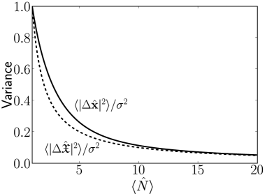
Figure 1: Deviation of the variance (relative to the wavepacket variance, $\sigma^{2}$) of the quasi intensive COM coordinate (dashed) from the true intensive COM coordinate (solid) for a heralded coherent state.

From the graphical comparison shown as Fig. 1 it is clear that the standard quantum noise limit for the extensive (quasi mean) position measurement is lower than that for the intensive position measurement. This can be understood as a consequence of the fact that an extensive position measurement for a coherent state effectively weights all individual particle position measurements equally. This is advantageous for a coherent state - as in a laser pulse - where all particles arrive independently, and carry the same information. However, not all pulses have the same number of independent particles. An intensive measurement weights all collective particle position measurements equally, regardless of particle number. This gives less weight per particle measurement when the particle number is large, and hence is less than optimal.

III.2 Fermionic fields

Identifying a characteristic COM uncertainty for a cold Fermi gas is a natural extension to the above discussion. We therefore consider a spin-polarized gas of $N$ identical fermions at zero temperature. In other words, we consider a system in which all modes below the characteristic Fermi energy contain a single fermion each, whilst those above this energy are vacant. Using the Hartree-Fock assumption of wavefunction factorization, this state can be written

$$|\Psi^{(N)}\rangle=\left(\prod_{j=0}^{N-1}\hat{a}_{j}^{\dagger}\right)\left|0\right\rangle$$ (33)

where the fermion creation operator for the j-th free-particle energy level is defined as

$$\hat{a}_{j}^{\dagger}=\int d^{D}\mathbf{x}\chi_{j}(\mathbf{x})\hat{\Psi}^{\dagger}(\mathbf{x})$$ (34)

and $\chi_{j}(\mathbf{x})$ is an orthonormal set of mode functions (energy eigenstate basis).

We now calculate the expectation value of the mean position variance operator given by Eq. 25. For the first term in this equation, we employ the commutation relation $\left[\hat{\Psi}(\mathbf{x}),\hat{a}_{j}^{\dagger}\right]{}_{+}=\chi_{j}(\mathbf{x})$ to show that

$$\hat{\Psi}(\mathbf{x})\left|\Psi^{(N)}\right\rangle=\sum_{j=0}^{N-1}(-1)^{j}\chi_{j}(\mathbf{x})\left|\Psi_{-j}^{(N)}\right\rangle$$ (35)

where $\left|\Psi_{-j}^{(N)}\right\rangle=\left(\prod_{k=0}^{N-1}\left(\hat{a}_{k}^{\dagger}\right)^{(1-\delta_{jk})}\right)\left|0\right\rangle$. Taking the inner product of this result with it’s conjugate leads to

$$\sigma^{2}=\frac{1}{N}\sum_{j=0}^{N-1}\int d^{D}\mathbf{x}\left\{\left|\Delta\mathbf{x}\right|^{2}\left|\chi_{j}(\mathbf{x})\right|\right\}.$$ (36)

To evaluate the second term in the expectation value of Eq. 25 we consider the action of two Fermi field operators on the system state vector:

$$\hat{\Psi}(\mathbf{y})\hat{\Psi}(\mathbf{x})\left|\Psi^{(N)}\right\rangle = \sum_{jk=1}^{N}(-1)^{j+k-\theta(k-j)}(1-\delta_{jk})$$ (37)

$$\times\chi_{j}(\mathbf{x})\chi_{k}(\mathbf{y})\left|\Psi^{(N)}\right\rangle$$

Again taking the norm of the result, we find:

$$\langle:|\mathbf{X}|^{2}:\rangle = \sum_{jk=1}^{N}\int d^{D}\mathbf{x}d^{D}\mathbf{y}\{\mathbf{x}\cdot\mathbf{y}[|\chi_{j}(\mathbf{x})|^{2}|\chi_{k}(\mathbf{y})|^{2}$$ (38)

$$-\chi_{j}^{*}(\mathbf{x})\chi_{k}(\mathbf{x})\chi_{k}^{*}(\mathbf{y})\chi_{j}(\mathbf{y})]\}$$

Up until now, the single particle basis $\chi_{j}(\mathbf{x})$ has been arbitrary. For definiteness, we will assume that the functions $\chi_{j}(\mathbf{x})=\langle\mathbf{x}|j\rangle$ are energy eigenstates of a simple harmonic oscillator of mass $m$ and frequency $\omega$. That is,

$$\sigma^{2} = \frac{1}{N}\sum_{j=0}^{N-1}\int d^{D}\mathbf{x}\{|\mathbf{x}|^{2}\langle j|\mathbf{x}\rangle\!\langle\mathbf{x}|j\rangle\}$$

$$= \frac{1}{N}\sum_{j=0}^{N-1}\langle j|\hat{\mathbf{q}}^{2}|j\rangle,$$

where we have also defined the first quantized position operator $\hat{\mathbf{q}}=(\hat{q}_{x},\hat{q}_{y},\hat{q}_{z})$ such that $\hat{q}_{\mu}|\mathbf{x}\rangle=x_{\mu}|x\rangle$. Recalling that this operator can also be expressed in terms of raising ($\hat{\alpha}_{\mu}^{\dagger}$) and lowering ($\hat{\alpha}_{\mu}$) operators, we find

$$\sigma^{2} = \frac{1}{N}\left(\frac{\hbar}{2m\omega}\right)\sum_{j=0}^{N-1}\sum_{\mu=1}^{D}(\langle j|\hat{\alpha}_{\mu}\hat{\alpha}_{\mu}^{\dagger}|j\rangle+\langle j|\hat{\alpha}_{\mu}^{\dagger}\hat{\alpha}_{\mu}|j\rangle$$

and hence the variance due to the wavepacket extent is in this case

$$\sigma^{2}=\frac{D\hbar}{2m\omega}N.$$ (39)

The normally ordered component of the COM variance can be evaluated using a similar approach. The first line in Eq. 38 vanishes due to the odd parity of the integrand. The remaining term gives

$$\langle:|\hat{\mathbf{X}}|^{2}:\rangle = -\sum_{jk=0}^{N-1}\sum_{\mu=1}^{D}\langle j|\hat{q}_{\mu}|k\rangle\!\langle k|\hat{q}_{\mu}|j\rangle$$

$$= -\frac{D\hbar}{2m\omega}\sum_{jk=0}^{N-1}\left((j+1)\delta_{j+1,k}+j\delta_{j-1,k}\right)$$

which after combining the two terms in brackets leaves

$$\langle:|\hat{\mathbf{X}}|^{2}:\rangle = -\frac{D\hbar}{2m\omega}N(N-1).$$ (40)

Taking into account spin degeneracy of an $S$-component Fermi gas, which gives rise to $S$ independent measurements each with $N/S$ particles, the COM variance for an $N$-particle Fermi gas at zero temperature held in an harmonic trap is

$$\langle|\Delta\hat{\mathbf{x}}|^{2}\rangle = \frac{S\sigma^{2}}{N^{2}}.$$ (41)

The contribution from the normally ordered term vanishes for $N=1$ and is less than zero for all $N>1$. As this term always vanishes for a bosonic number state, while the wavepacket variance is identical for a bosonic gas constrained to the same density profile as the fermionic gas we have just considered (i.e. $\langle\hat{n}(\mathbf{x})\rangle=\sum_{j=1}^{N}|\chi_{j}(\mathbf{x})|^{2}$), it is clear that the standard quantum limit for COM measurements is intrinsically lower for fermions than for bosons. In the case of a harmonic trap, the variance is $N$ times smaller for fermions than for bosons.

IV Quantum wave packet spreading

In pure state evolution, any increase in the uncertainty above the standard quantum limit is regarded as originating in quantum wave-packet spreading of the center-of-mass. We thus define

$$\sigma_{QM}=\sqrt{\langle\Delta\mathbf{\mathfrak{X}}^{2}\rangle-\sigma_{SQL}^{2}}$$ (42)

to measure this phenomenon. We note that states for which $\sigma_{QM}\gg 0$ are the “strange quantum states” which are mentioned in the photonic case by some previous workersFiniHagelstein , and also play a role in the theory of quantum non-demolition position measurements and gravity-wave detection. This must be carefully distinguished from uncertainties in mixed states, which are not caused by quantum superpositions.

A similar property to quantum wave-packet spreading is already known, and observed experimentally. In the Gordon-Haus effectGordon in amplifying optical fibers, the soliton time-of-arrival is perturbed by the effect of laser amplification. Soliton timing jitter of this type is an extrinsic property of the amplifying system. Instead, we will treat the intrinsic quantum effects which are present even in the absence of the spontaneous emission noise of a laser amplifier.

To solve for the time evolution of the COM uncertainty of arbitrary states, we first note that Eq. 4 can be directly integrated to give the following result, for any (effectively non-relativistic) system prepared in an eigenstate of the total particle number operator:

$$\hat{\mathbf{x}}_{N}(t)=\hat{\mathbf{x}}_{N}(0)+t\frac{\hat{\mathbf{P}}}{mN}.$$

where $m$ can be either the mass of an atom or the effective mass of a polariton, as discussed in section II.1 above. For extreme relativistic or massless photon propagation, the lack of a longitudinal dispersion mechanism implies that wave-packet spreading is analogous to diffraction, and occurs transversely to the propagation direction. This must be treated using the conserved number density current operator of Eq. (10).

This result can be generalized to other states, provided that the total number is conserved during the evolution. Under this condition, the Heisenberg picture evolution of the intensive and quasi-intensive mean position operators are respectively

$$\hat{\mathbf{x}}(t)=\hat{\mathbf{x}}(0)+t\frac{\hat{\mathbf{P}}}{m\hat{N}},\,\,\textrm{and}$$ (43)

$$\hat{\mathbf{\mathfrak{X}}}(t)=\hat{\mathbf{\mathfrak{X}}}(0)+t\frac{\hat{\mathbf{P}}}{m\langle\hat{N}\rangle}.$$ (44)

In the pulse frame, taking the squares gives the evolution of the (true intensive and quasi intensive) mean position:

$$\langle|\Delta\hat{\mathbf{x}}(t)|^{2}\rangle = \langle|\hat{\mathbf{x}}(0)|^{2}\rangle+\frac{t}{m}\langle(\hat{\mathbf{x}}(0)\cdot\hat{\mathbf{P}}+\hat{\mathbf{P}}\cdot\hat{\mathbf{x}}(0))/\hat{N}\rangle$$ (45)

$$+\frac{t^{2}}{m^{2}}\langle|\hat{\mathbf{P}}|^{2}/\hat{N}^{2}\rangle,\,\,\textrm{and}$$

$$\langle|\Delta\hat{\mathbf{\mathfrak{X}}}(t)|^{2}\rangle = \langle|\hat{\mathbf{\mathfrak{X}}}(0)|^{2}\rangle+\frac{t}{m}\langle\hat{\mathbf{\mathfrak{X}}}(0)\cdot\hat{\mathbf{P}}+\hat{\mathbf{P}}\cdot\hat{\mathbf{\mathfrak{X}}}(0)\rangle/\langle\hat{N}\rangle$$ (46)

$$+\frac{t^{2}}{m^{2}}\langle|\hat{\mathbf{P}}|^{2}\rangle/\langle\hat{N}\rangle^{2}.$$

IV.1 Bosonic coherent state evolution

When the system is initially prepared in a coherent state (projected to remove the vacuum state, as in Eq. 30) the mean position uncertainties evolve as

$$\langle|\Delta\hat{\mathbf{\mathfrak{X}}}(t)|^{2}\rangle_{P}=\frac{1}{\langle\hat{N}\rangle_{P}}\left[\alpha+\beta\frac{\hbar t}{m}+\gamma\left(\frac{\hbar t}{m}\right)^{2}\right]$$ (47)

where $\alpha,\beta,\gamma$ are functions of the initial wave-packet shape only. These are given by:

$$\alpha = \int|\mathbf{x}|^{2}|\chi(\mathbf{x})|^{2}d^{D}\mathbf{x}$$

$$\beta = i\int\mathbf{x}\cdot\left[(\nabla\chi^{*}(\mathbf{x}))\chi(\mathbf{x})-\chi^{*}(\mathbf{x})(\nabla\chi(\mathbf{x}))\right]d^{D}\mathbf{x}$$

$$\gamma = \int|\nabla\chi(x)|^{2}d^{D}\mathbf{x}$$

where $\chi(\mathbf{x})$ is again the normalized spatial mode in the co-moving frame.

This result agrees with previous approximate linearized results obtained for initial coherent solitonsLai , but is much more general. It is valid for any initial coherent state, at large photon number, independent of the nonlinear interaction, due to the fact that the coefficients depend only on the initial coherent state. If we recall that the Hamiltonian corresponds to coupled propagation of massive bosons, then the reason for this exact independence of the coupling is transparent. The definition of $\hat{\mathbf{\mathfrak{X}}}$ corresponds to a center-of-mass measurement, which never depends on the two-body coupling. However, the standard quantum limit does depend on the nonlinearity. This is because the coupling changes the pulse-shape $\langle\hat{\Psi}^{\dagger}(\mathbf{x})\hat{\Psi}(\mathbf{x})\rangle$, as an initially coherent pulse with uncorrelated bosons evolves into a correlated state. Thus, for example, if a 1D coherent source produces a sech input pulse, so that $\chi(x)=\mbox{sech}(x/2)/2$, then $\alpha=\pi^{2}/3\,{\,\textrm{m}}^{2};\beta=0;\,\,\gamma=1/12\,\,\textrm{m}^{-2}$. This is not a minimum uncertainty state, as:

$$\langle\Delta{\hat{\mathbf{\mathfrak{X}}}(0)}^{2}\rangle_{P}\langle\Delta\hat{P}^{2}\rangle_{c}=\pi^{2}/36=0.27415..>0.25.$$ (48)

Coherent Gaussian input pulses, on the other hand, are a minimum uncertainty state in momentum and position, as one might expect. However, these have a large continuum radiation when used to form solitons. This leads to a paradox: the sech-type coherent soliton has a larger uncertainty product than a coherent Gaussian pulse, yet experimentally appears more localized!

More complex input states than coherent states can be considered, and they also can be treated exactly. For example, Haus and LaiLai have considered an input state of spatially correlated photons, consisting of a superposition of eigenstates of the interacting Hamiltonian. In this case, the mean pulse-shape is a sech pulse. However, due to boson-boson correlations, the resulting state is a minimum uncertainty state in position and momentumKartner . It is unlikely that any existing laser source can produce the required correlations. Nevertheless, this example shows that, when dealing with correlated states, it is possible to reach the minimum uncertainty limit with a non-Gaussian pulse-shape.

V Soliton propagation

We next consider weakly interacting particle distributions confined to a single transverse mode of a waveguide, which can therefore be treated by an effective one dimensional field theory. Examples of such systems include photonic wave packets in single-mode optical fibers and atomic BEC clouds moving in 1D wave guides. Such physical systems have the property that they can form solitons, in which the classical wave-packet spreading is minimized, thus forming excellent candidates for observation of these center-of-mass uncertainties.

V.1 Effective field theory

Our starting point is the standard Hamiltonian operator describing a 1D ensemble of spinless bosons which interact through a simple delta-function potential. In terms of a dimensionless particle density amplitude, $\hat{\phi}$, the Hamiltonian can be written:

$$\hat{H}=\frac{1}{2}\int d\zeta\left[\hat{\phi}_{\zeta}^{\dagger}(-\partial_{\zeta}^{2})\hat{\phi}_{\zeta}\pm\hat{\phi}_{\zeta}^{\dagger 2}\hat{\phi}_{\zeta}^{2}\right]$$ (49)

where the field operators have the commutation relation

$$[\hat{\phi}_{\zeta}(\tau),\hat{\phi}_{\zeta^{\prime}}^{\dagger}(\tau)]=\frac{1}{\bar{n}}\delta(\zeta-\zeta^{\prime}).$$ (50)

Heisenberg’s equations of motion for the field operators are then

$$i\partial_{\tau}\hat{\phi}_{\zeta}=\bar{n}[\hat{\phi}_{\zeta},\hat{H}].$$ (51)

These equations simultaneously describe at least two physically distinct many-body systems, the details of which are implicit in the characteristic time $t_{0}=t/\tau$ and length $x_{0}=x/\zeta$ which link the physical and dimensionless coordinate systems. Together with the mean particle number $\bar{n}$ and the sign of the nonlinearity, these scaling factors completely specify a particular system.

Loss (or gain) mechanisms can be formally incorporated into this model by including terms in the Hamiltonian which couple the system to external degrees of freedom. After tracing over these reservoir states, this procedure leads to a master equation for the reduced density operator in generalized Lindblad form, which includes c-number damping coefficients. Although these are frequently added in an ad hoc fashion, it is important to note that in doing so one implicitly assumes that the reservoir is at very low temperature and has no thermal contribution to the system modes.Carmichael

V.2 Numerical results

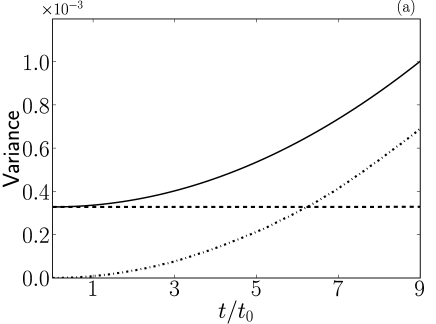
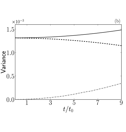
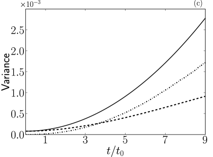
Figure 2: Mean position variances for 1D coherent pulses of $\bar{n}=10^{4}$ particles propagating in a dispersive medium. The three figures correspond to three different wavepacket shapes: (a) the soliton solution to the 1D nonlinear Schrödinger equation $\langle\hat{\phi}(\zeta)\rangle=\frac{1}{2}\textrm{sech}(\frac{1}{2}\zeta)$, (b) a wider pulse of the form $\langle\hat{\phi}(\zeta)\rangle\propto\textrm{sech}(\frac{1}{4}\zeta)$ and (c) a narrower pulse $\langle\hat{\phi}(\zeta)\rangle\propto\textrm{sech}(\zeta)$. The solid lines represents the analytically determined total variance $\langle\Delta\hat{\mathbf{\mathfrak{X}}}^{2}\rangle/x_{0}^{2}$, while the dashed and dash-dotted lines represent the numerical results for the classical ($\sigma_{SQL}^{2}/x_{0}^{2}$) and quantum ($\sigma_{QM}^{2}/x_{0}^{2}$) contributions respectively.

Typical results for the mean position variances during the propagation of a $10^{4}$ particle coherent state soliton with initial shape $\langle\hat{\phi}_{\zeta}\rangle=\frac{1}{2}\mbox{sech}(\frac{1}{2}\zeta)$ are shown in Fig. 2(a). Here the dashed line represents the analytic solution for the total variance $\langle\Delta\hat{\mathbf{\mathfrak{X}}}^{2}\rangle/x_{0}^{2}$, while the solid lines are numerical results generated using a stochastic computer simulation equivalent to the quantum nonlinear Schr dinger equationCarter . These results include the total variance (in complete agreement with the analytical result), the standard quantum limit $\sigma_{SQL}^{2}$ and the measure of quantum wave packet spreading $\sigma_{QM}^{2}$. For comparison, Figs. 2(b) and 2(c) display the evolution of these variances for wider and narrower pulses than the classical soliton solution.

The standard quantum limit for the soliton is constant, which indicates each soliton envelope remains nearly invariant; as one might expect from a classical analysis. This is a remarkable macroscopic quantum effect. An optical coherent state soliton consists of linear superpositions of continuum photons and different number-momentum eigenstates. This is clearly different to a classical soliton with frequency jitter, yet it behaves very similarly as far as the center position is concerned. On the other hand, the standard quantum limit for a pulse in a linear medium increases in the same way as the soliton quantum wave-packet spreading, due to the dispersive spreading in the average intensity. In the linear case, an initial coherent state remains coherent, so the increased quantum positional uncertainty can be attributed to the shot-noise error intrinsic to the detection of a pulse whose envelope is not sharply localized.

This indicates that the intrinsic quantum wave-packet spreading can be observed only for the soliton, where it is easily distinguishable from coherent shot-noise effects. However, this does not mean that a quantum soliton is unstable. Each soliton preserves its soliton pulse shape. In this sense, the soliton quantum diffusion is different from the classical pulse broadening due to linear dispersion. In fact, in the case of the correlated initial state, the second-order and the fourth-order correlation functions are invariantKousnetsov .

VI Practical examples

In this section we consider some practical examples and numerical estimates with currently available experimental technologies.

VI.1 Photonic systems

In the optical case, the soliton propagation model describes a distribution of interacting photons (or strictly, polaritons) propagating in a single-mode fiber with a third-order Kerr nonlinearity, $\chi^{(3)}$. Here the sign of the interaction term is positive for normal dispersion and negative for anomalous dispersion. For $\chi^{(3)}$ soliton propagation, we require the carrier frequency to be inside the anomalous dispersion regime.

Typical orders of magnitude of soliton parameters are $\bar{n}=10^{9}$, $t_{0}=10^{-12}$s, $x_{0}=1$m. With these parameters, we obtain a standard quantum limit of $10^{-8}$m for a single coherent pulse. In $1$km of propagation, the wave packet would therefore spread to $10^{-5}$m, much greater than the standard quantum limit. Although still less than the actual soliton extent of $10^{-4}$m, this is a remarkably large quantum wave-packet spreading in a composite object of $10^{9}$ particles. An experiment on quantum-mechanical wave-packet spreading in a composite object of this type (such as that described in FiniHagelstein ) would test quantum mechanics in a region of much larger particle number than previously achieved.

Unfortunately, however, even fiber attenuations lower than the usual $0.1$dB/km translate to losses of over $10^{7}$ photons from such a pulse over this distance. Since each particle lost can be used to obtain information about the mean position of a pulse, these losses would destroy the coherence properties of a wave packet. Even so, the remaining statistical uncertainty is a practical concern – it is, for example, likely to have a severe effect on the error-rate in pulse-position logicIslam . The effect may be enhanced by using dispersion-engineered fibersFiniHagelstein .

VI.2 Degenerate Bose gasses

The same effective field theory can also describe a dilute, single-species gas of massive bosonic particles, interacting through low-energy S-wave ($l=0$) scattering events and held in a potential which confines the particles to a single transverse mode but allows longitudinal propagation. In this case, one finds that:

$$x_{0} = \frac{\hbar^{2}}{m\bar{n}g_{1D}}$$

$$t_{0} = \frac{\hbar^{3}}{m\bar{n}^{2}g_{1D}^{2}}$$ (52)

where $m$ is the single-particle mass, and $g_{1D}=2\hbar a_{s}\omega_{\perp}$ is the effective 1D interaction strengthAbdullaev . For temperatures well below the BEC transition temperature, such gasses are usually considered to be the matter-wave analog of coherent laser output, and are thus sometimes referred to as atom-lasers.

Although there are various paths one can take to realizing matter-wave solitons, we consider here only bright solitons in the absence of any periodic potential – i.e., solitons for which the required nonlinearity is provided by an attractive interaction between atoms. Such solitons have been observedHulet ; Salomon in BECs of ⁷Li atoms, where the presence of a Feshbach resonance is used to tune the effective scattering length from repulsive to attractive. These experiments present the very real possibility of directly observing the quantum dispersion of a mesoscopic object composed of massive particles, thanks to the extremely slow rate of atom loss from these systems . For instance, the total predicted loss rate for a trapped cloud of attractive ⁷Li atoms of roughly the same number as that in Salomon is around $50/$s.Pozzi (This is analogous to an optical pulse traveling along a fiber with an attenuation of less than $10^{-6}$dB/km!)

Drawbacks in dealing with atomic clouds include the effect of finite temperatures. This places a classical uncertainty in the center of mass momentum and therefore leads to a classical spread in center of mass position over time, obscuring the quantum diffusion. For a 1D gas of $N$ bosons of mass $m$ and temperature $T$, the equipartition theorem gives

$$\dot{\sigma}_{th}=\sqrt{\frac{k_{B}T}{mN}}$$ (53)

where $\dot{\sigma}_{th}$ is the linear rate of increase in the thermal mean position uncertainty.

For example, using numbers from the experiment of Khaykovich et al.Salomon and assuming a condensate temperature of $0.5T_{c}\simeq 80$nK we find that the standard deviation in the mean position due to thermal noise increases linearly at a rate of $1.3\times 10^{-4}$m/s. This is quite fast, when compared to the effect of quantum spreading of the soliton wave packet, which increases the standard deviation at the much slower rate of $4.2\times 10^{-5}$m/s. As this is an order of magnitude smaller than the thermal uncertainty, whose growth rate goes as the square root of the cloud temperature, this implies that temperatures less than $1$nK are required to directly observe quantum wave packet spreading. Although this is well below what is achieved in current ⁷Li experiments, Leanhardt et al.Ketterle have achieved temperatures of less than $0.5$nK in condensates of spin-polarized ²³Na, indicating that it may not be impossible to achieve such low temperatures in matter-wave soliton experiments. We note that adiabatic changes in the interaction strength could be used to compress the soliton, thereby increasing the quantum position uncertainty relative to the standard quantum limit.

VI.3 Degenerate Fermi gasses

Ultra-cold degenerate Fermi gases have recently been obtained in several laboratoriesformation ; Helium3 . The prospects for fermionic solitons have not yet been established clearly, although tunable Feshbach resonances with both attractive and repulsive interactions are known to exist. The species observed experimentally include ${}^{40}K$ , ${}^{6}Li$ and ${}^{3}He^{*}.$ Atom correlationsJin have already been experimentally observed in optical measurements with ${}^{40}K$. One of the most interesting cases is metastable fermionic Helium, in which atoms can be counted directly using multi-channel plate detectorsHelium3 . This affords an interesting possible avenue to testing the prediction that center-of-mass fluctuations are reduced for fermions relative to bosons.

VI.4 Double-slit interference of soliton ‘particles’

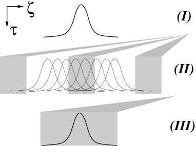
Figure 3: Possible soliton double slit interference experiment. The soliton wave packet (I) broadens over time due to the linear increase in the quantum uncertainty in the mean position. Lasers then eliminate solitons outside of two ‘slits’ (II). Any remaining soliton is left to propagate until it undergoes absorption imaging (III).

Provided one could overcome this difficulty, it would be extremely interesting to conduct double slit interference experiments with such large quantum objects. One possible implementation of this idea – essentially an atomic implementation of the fiber experiment proposal in FiniHagelstein – is shown in schematic as Fig. 3. Here a matter-wave soliton is allowed to propagate without disturbance until its quantum wave packet is large compared with the soliton width. A tightly focused laser pulse is then used to remove the central and outer elements of the distribution, effectively creating a pair of apertures through which the remaining components of the distribution pass. At some later time, the distribution is imaged and the mean position of the soliton measured. Another approach - provided the separation was large compared to the soliton size - would be to use temporal switching of a localized reflective potential, in order to only affect one part of the quantum soliton superposition. Averaging over many shots should then produce an interference pattern with any thermal effects being manifest as a loss in fringe visibility.

One of the primary challenges one would face in conducting this experiment would be addressing the fact that its duration needs to be less than the average particle lifetime in order to maintain coherence, while still long enough to allow sufficient quantum wave packet spreading. A possible solution might be to use a blue-detuned laser to provide a small repulsive potential near the center of the wave packet to enhance the broadening and thereby reduce the length of time required to produce an interference pattern. This technique might also allow one to forgo the use of destructive laser pulses to create the apertures by instead relying on this repulsive potential to separate the center of mass wave packet into two components. Another technique which appears possible, is to employ the recently proposed soliton quantum beam-splitterLeeBrand to initially separate two quantum soliton components based on their velocities, prior to subsequent recombination.

A related challenge would be resolving the resulting fringes, as their width is inversely proportional to particle number and limited by the trap lifetime through the maximum length of the experiment. (This can be shown by treating the soliton as a de Broglie wave of mass $mN$; $m$ and $N$ being the single-particle mass and the total number of constituent atoms respectively.)

Despite these issues, such an interference pattern would provide smoking gun evidence that quantum mechanical superpositions of massive composite objects of mesoscopic scale had been achieved.

VII Summary

In summary, quantum wave-packet spreading is a remarkable macroscopic quantum effect. It provides a fundamental limit - independent of amplifier noise - both to high-speed communications in dispersive waveguides, and to applications of atom lasers. Since it provides a means by which quantum mechanics can couple to the gravitational field, it may also provide a route to new tests of quantum mechanics. Of more practical interest is the fact that the standard quantum limit for center-of-mass measurement variance is highly sensitive to particle statistics. It is decreased by a factor of $N$ when the particle statistics are fermionic. This appears testable in atom-counting experiments with meta-stable ${}^{3}He$ .

- (1) B. Brezger, L. Hackerm ller, S. Uttenthaler, J. Petschinka, M. Arndt, and A. Zeilinger, Phys. Rev. Lett. 88, 100404 (2002).
- (2) L. Landau and R. Peierls, Z. Phys. 69, 56 (1931).
- (3) K. Watanabe, H. Nakano, A. Honold and Y. Yamamoto, Phys. Rev. Lett. 62, 2257 (1989); H. A. Haus, K. Watanabe and Y. Yamamoto, J. Opt. Soc. Am. B6, 1138 (1989).
- (4) Y. Lai and H. A. Haus, Phys. Rev. A40, 844 (1989); H. A. Haus and Y. Lai, J. Opt. Soc. Am. B7, 386 (1990).
- (5) J. M. Fini and P. L. Hagelstein, Phys. Rev. A 66, 033818 (2002).
- (6) S. J. Carter, P. D. Drummond, M. D. Reid and R. M. Shelby, Phys. Rev. Lett. 58, 1841 (1987); P. D. Drummond and S. J. Carter, J. Opt. Soc. Am. B4, 1565 (1987).
- (7) P. D. Drummond and J. F. Corney, J. Opt. Soc. Am. B 18, 139 (2001).
- (8) M. Rosenbluh and R. M. Shelby, Phys. Rev. Lett. 66, 153 (1991).
- (9) P. D. Drummond, R. M. Shelby, S. R. Friberg and Y. Yamamoto, Nature 365, 307 (1993).
- (10) J. F. Corney, P. D. Drummond, J. Heersink, V. Josse, G. Leuchs and U. L. Andersen, Phys. Rev. Lett. 97, 023606 (2006).
- (11) S. R. Friberg, S. Machida, Y. Yamamoto, Phys. Rev. Lett. 69, 3165 (1992).
- (12) L. Diosi, Phys. Rev. A 40 (1989) 1165.
- (13) G. C. Ghirardi, R. Grassi, and A. Rimini, Phys. Rev. A 42, 1057 (1990)
- (14) R. Penrose, Gen. Rel. Grav. 28, 581 (1996).
- (15) G. ’t Hooft, Class. Quant. Grav. 16, 3263 (1999).
- (16) K. P. Tod, Physics Letters A 280, 173 (2001).
- (17) S. De Filippo and F. Maimone, Phys. Lett. B 584, 141 (2004).
- (18) M. D. Reid, Zeitschrift fur Naturforschung A-A: J. Physical Sci. 56, 220 (2001); M. D. Reid and E. G. Cavalcanti, J. Mod. Optics 52, 2245 (2005); E. G. Cavalcanti and M. D. Reid, Phys. Rev. Lett. 97, 170405 (2006).
- (19) Y. Aharonov, D. Z. Albert, L. Vaidman, Phys. Rev. Lett. 609, 1351 (1988).
- (20) M. I. Kolobov, Rev. Mod. Phys. 71, 1539 (1999).
- (21) N. Treps, N. Grosse, W. P. Bowen, C. Fabre, H. A. Bachor and P. K. Lam, Science 301, 940 (2003).
- (22) P. D. Drummond, Phys. Rev. A60, R3331 (1999); J. Phys. B 39, S573 (2006).
- (23) J. P. Gordon and H. A. Haus, Opt. Lett. 11, 665 (1986).
- (24) P. D. Drummond and A. D. Hardman, Europhys. Lett. 21, 279 (1993).
- (25) D. Yao, Phys. Rev. A52, 4871 (1995).
- (26) R. J. Glauber, Phys. Rev. 130, 2529 (1963).
- (27) F. X. Kartner and L. Boivin, Phys. Rev. A53, 454 (1996).
- (28) M.N. Islam, C.E. Soccolich, J.P. Gordon, Opt. Quantum Electron. (UK) 24, 1215-1235 (1992); P. D. Drummond and W. Man, Optics Comms 105, 99 (1994); J. F. Corney and P. D. Drummond, JOSA B 18, 153 (2001).
- (29) D. Yu Kouznetsov, Quantum Optics 4, 221 (1992).
- (30) F. Kh. Abdullaev and J. Garnier, Phys. Rev. A 70, 053604 (2004).
- (31) H. J. Carmichael, Statistical Methods in Quantum Optics I, 16 (1999).
- (32) L. Khaykovich, F. Schreck, G. Ferrari, T. Bourdel, J. Cubizolles, L. D. Carr, Y. Castin and C. Salomon, Science 296, 5571 (2002).
- (33) K. E. Strecker, G. B. Partridge, A. G. Truscott and R. G. Hulet, Nature 417, 150 (2002).
- (34) B. Pozzi, L Salasnich, A. Parola and L. Reatto, J. Low Temp. Phys. 119, 57 (1999).
- (35) A. E. Leanhardt, T. A. Pasquini, M. Saba, A. Schirotzek, Y. Shin, D. Kielpinski, D. E. Pritchard and W. Ketterle, Science 301, 1513 (2003).
- (36) C. A. Regal, M. Greiner, and D. S. Jin, Phys. Rev. Lett. 92, 040403 (2004); M. W. Zwierlein et al., Phys. Rev. Lett. 92, 120403 (2004); M. Bartenstein et al., Phys. Rev. Lett. 92, 120401 (2004); T. Bourdel et al., Phys. Rev. Lett. 93, 050401 (2004).
- (37) W. Vassen, T. Jeltes, J. M. McNamara and A. S. Tychkov, cond-mat/0610414.
- (38) M. Greiner, C.A. Regal, C. Ticknor, J.L. Bohn, and D. S. Jin, Phys. Rev. Lett. 92, 150405 (2004).
- (39) C. Lee and J. Brand, Europhys. Lett., 73, 321 (2006).