Ferromagnetic Relaxation by Magnon Induced Currents

Abstract

A theory for calculating spin wave relaxation times based on the magnon-electron interaction is developed. The theory incorporates a thin film geometry and is valid for a large range of magnon frequencies and wave vectors. For high conductivity metals such as permalloy, the wave vector dependent damping constant approaches values as high as $0.2$, showing the large magnitude of the effect, and can dominate experimentally observed relaxation.

One of the fundamental problems of magnetism is to determine a mechanism for dissipation of energy in a system subject to a change in the direction of the external magnetic field. Historically, these ferromagnetic relaxation processes have been explored by ferromagnetic resonance (FMR) in which the absorption of a small RF frequency field applied perpendicular to a large DC field is measured. More recently, direct measurement of large angle switching has been made by multiple groups HSF1997PRL ; Choi2001PRL ; AB2000Sci . Time resolved Kerr microscopy has made it possible to track isolated magnetic relaxation processes with picosecond temporal resolution HSF1997PRL and also to image the individual components of the precessing magnetization AB2000Sci . It has been previously shown that for many examples of large angle switching, particularly those involving materials with large magnetizations, the dominant relaxation process is very different than that applicable to FMR. In particular, it was found that the coherent mode scatters with thermal magnons to form two $k\neq 0$ magnons DV2003PRL . This 4-magnon process rapidly escalates as the $k\neq 0$ magnon levels are populated, thus promoting additional scattering. This previous work thus accounted for the rapid movement of the magnetization into the new direction, but the dissipation of the magnetic energy stored in the $k\neq 0$ modes still must be addressed.

In a conducting ferromagnet the interaction between the conduction electrons and the magnons become very important. The magnetic field generated by the spin wave is time dependent and therefore, by Faraday’s law, it creates an electric field in the system. These electric fields, unlike conventional eddy currents, are wave like in nature. In a metallic system, the fields drive the conduction electrons. These magnon induced currents help dissipate the energy of the system by Joule heating. Abrahams A1955PR addressed this question half a century ago by taking into account the interaction between spin waves and conduction electrons. However, his bulk estimates predicted relaxation times one order of magnitude less than required to explain FMR line widths. Subsequently several attempts have been made to give a consistent theory of ferromagnetic relaxation from the point of view of an FMR experiment KP1975PRB . Later, Almeida and Mills AM1996PRB explored the same interaction and derived the Green’s function for the limited case of small angle precession in the absence of quantum mechanical exchange, i.e. in the long wavelength limit.

In the present work, we avoid much of the limitations found in previous work. Solution of the general problem is difficult because the magnon-induced currents generate new fields which further affect magnons and create new currents. Here we show that expansion in the small parameter $4\pi\omega\sigma/c^{2}k^{2}$ allows an explicit solution to the general problem. It allows prediction of decay rates for magnons of arbitrary frequency and large amplitudes that are limited only by the Holstein Primakoff transformation HP1940PR . In particular, it can be applied to the problem of magnons generated by four-magnon scattering after a large angle rotation such is common in modern switching experiments and technological applications such as magnetic recording. We also discuss our results in context of the spin wave resonance experiments capable of measuring the linewidth of the higher order $k$ modes. Historically, these experiments were used to measure the exchange constant of the material.

We consider an infinite film of thickness $d$ made of ferromagnetic metal. The top and the bottom surfaces of the film are at $z=d$ and $z=0$ respectively (see Fig. 1). A spin wave of wave vector $\mathbf{k}=k\widehat{x}$ and frequency $\omega$ is excited in the system.

We write the electric and magnetic fields in the system as a series expansion

$$\mathbf{E} = \sum_{n=0}^{\infty}\left(\frac{4\pi\sigma\omega}{c^{2}k^{2}}\right)^{n}\mathbf{E}^{(n)}$$

$$\mathbf{H} = \sum_{n=0}^{\infty}\left(\frac{4\pi\sigma\omega}{c^{2}k^{2}}\right)^{n}\mathbf{H}^{(n)}$$ (1)

where $\sigma$ is the conductivity of the medium and $c$ is the velocity of light. For typical frequency and wave vector, this expansion parameter is quite small, e.g. $10^{-4}$ for Fe ($\sigma=9\times 10^{16}$ s^-1). Therefore, the series converges rapidly and only the leading term has practical interest. The $n-$th order terms in the expansion of Eq. (1) obey the Maxwell equations

$$\nabla\cdot\mathbf{E}^{(n)} = 0$$

$$\nabla\cdot(\mathbf{H}^{(n)}+4\pi\mathbf{M}\delta_{n0}) = 0$$

$$\nabla\times\mathbf{E}^{(n)} = -\frac{1}{c}\frac{\partial\mathbf{B}^{(n)}}{\partial t}$$

$$\nabla\times\mathbf{H}^{(n+1)} = \frac{4\pi\sigma}{c}\mathbf{E}^{(n)}$$

We neglect the displacement current in the last expression owing to $\omega\ll\sigma$. From Eq. (LABEL:eq:maxwell) $\nabla\times\mathbf{H}^{(0)}=0$, so we can write the magnetic field as the gradient of a magnetic scalar potential: $\mathbf{H}^{(0)}=-\nabla\phi_{\mathrm{M}}$. The scalar potential has a volume and a surface term and the zeroth order magnetic field produced by the spin waves can be written as Jackson

$$\mathbf{H}^{(0)} = -\int_{V}d^{3}r^{\prime}\frac{\mathbf{\nabla}\cdot\mathbf{M}(\mathbf{r^{\prime}})(\mathbf{r}-\mathbf{r^{\prime}})}{\left|\mathbf{r}-\mathbf{r^{\prime}}\right|^{3}}$$ (3)

$$+ \int_{S}d^{2}r^{\prime}\frac{\hat{n}\cdot\mathbf{M}(\mathbf{r^{\prime}})(\mathbf{r}-\mathbf{r^{\prime}})}{\left|\mathbf{r}-\mathbf{r^{\prime}}\right|^{3}}$$

where $\mathbf{M}$ is the magnetization of the sample and $\hat{n}$ is the outward normal to the surface carrying magnetic charge. We shall consider films to be thin enough that the spin waves are confined to the $x-y$ plane only. We shall consider two specific cases: $\mathbf{k}\bot\mathbf{M}$ and $\mathbf{k}\|\mathbf{M}$.

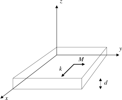
Figure 1: Schematic diagram showing the geometry used in the paper. An infinite ferromagnetic metallic slab with thickness $d$ along the $z$-direction is magnetized in-plane by applying an external field $\mathbf{H}$. We consider spin waves with wave vector $k$ propagating parallel to the surfaces.

We consider the spin wave propagating along the $x$ direction in the thin film. In configuration I, the magnetization is precessing in the $x-z$ plane

$$\mathbf{M}^{\mathrm{I}}=M_{0}\widehat{y}+\epsilon\left[\cos\left(kx-\omega t\right)\widehat{x}+\sin\left(kx-\omega t\right)\widehat{z}\right]$$

where $M_{0}$ is the component of magnetization perpendicular to the plane of precession and $\epsilon$ is the amplitude of precession. In our calculation, we need not restrict $\epsilon$ to be small compared to $M_{0}$. The zeroth order magnetic field from Eq. (3) for this configuration is

$$H_{x}^{\mathrm{I}(0)} =4\epsilon\pi\cos(kx-\omega t)\left[e^{-kz}-1\right]\; \mathrm{for}\>k >0$$

$$=4\epsilon\pi\cos(kx-\omega t)\left[e^{-k(z-d)}-1\right]\; \mathrm{for}\>k <0$$

$$H_{y}^{\mathrm{I}(0)} =0\quad$$

$$H_{z}^{\mathrm{I}(0)} =-4\epsilon\pi\sin(kx-\omega t)e^{-kz}\,\; \mathrm{for}\>k >0$$

$$=-4\epsilon\pi\sin(kx-\omega t)e^{-k(z-d)}\,\; \mathrm{for}\>k <0$$

According to Eq. (LABEL:eq:maxwell) $\mathbf{H}^{\mathrm{I}(0)}$ generates an electric field $\mathbf{E}^{\mathrm{I}(0)}$ which has only one nonzero component

$$E_{y}^{\mathrm{I}(0)} =\frac{2\xi}{k}\sin(kx-\omega t)[1-e^{-kz}]\quad \mathrm{for}\,k>0$$

$$E_{y}^{\mathrm{I}(0)} =\frac{2\xi}{k}\sin(kx-\omega t)[1-e^{-k(z-d)}]\quad \mathrm{for}\,k<0$$

where $\xi=2\pi\epsilon\omega/c$. Note the asymmetry of the solution for positive and negative values of $k$. The profile of the electric field for $k>0$ and $k<0$ are mirror symmetric with respect to $z=d/2$.

In configuration II, the magnetization is precessing in the $y-z$ plane

$$\mathbf{M}^{\mathrm{II}}=M_{0}\widehat{x}+\epsilon\left[\cos\left(kx-\omega t\right)\widehat{y}+\sin\left(kx-\omega t\right)\widehat{z}\right]$$

Since $\nabla\cdot\mathbf{M}^{\mathrm{II}}=0$ only the surface term of Eq. (3) contributes to the magnetic field given by (for $k>0$)

$$H_{x}^{\mathrm{II}(0)} = -2\epsilon\pi\cos(kx-\omega t)[e^{k(z-d)}-e^{-kz}]$$

$$H_{y}^{\mathrm{II}(0)} = 0$$

$$H_{z}^{\mathrm{II}(0)} = -2\epsilon\pi\sin(kx-\omega t)[e^{k(z-d)}+e^{-kz}]$$

which generates an electric field

$$E_{x}^{\mathrm{II}(0)} = \left[-Ae^{kz}+Be^{-kz}\right]\sin(kx-\omega t)$$

$$E_{y}^{\mathrm{II}(0)} = \frac{\xi}{k}\left[2-e^{k(z-d)}-e^{-kz}\right]\sin(kx-\omega t)$$

$$E_{z}^{\mathrm{II}(0)} = \left[Ae^{kz}+Be^{-kz}-\frac{2\xi}{k}\right]\cos(kx-\omega t)$$ (5)

where $A=(\xi/k)[(1-e^{-kd})/\sinh(kd)]$ and $B=(\xi/k)[(e^{kd}-1)/\sinh(kd)]$. Note that unlike in the previous configuration the components of the electric field are symmetric with respect to the two surfaces.

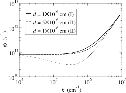
Figure 2: Dispersion relation for configurations I and II according to Eqs. (8) and (LABEL:eq:omegamag) for an infinite iron slab using $M_{S}=1700$ emu/cc, $A$ = $2\times 10^{-6}$ erg/cm, $\gamma$ = $1.76\times 10^{7}$ (Oe s)^-1 and $H_{\mathrm{ext}}=1000$ Oe.

The energy stored in the form of spin waves is dissipated from the system by the current generated by the electric field induced by the precessing spins. This induced electric field drives the free electrons in the metal to produce the magnon induced current. The ohmic power loss per unit volume due to this magnon induced current can be written as

$$P=\lim_{L\rightarrow\infty}\frac{\sigma}{2Ld}\int_{0}^{d}dz\int_{-L}^{+L}dx\left(E_{x}^{2}+E_{y}^{2}+E_{z}^{2}\right)$$

Integrating over the square of the electric field described in Eqs. (LABEL:eq:EI) and (5), we obtain the power dissipation per unit volume

$$P^{\mathrm{I}}(k,d) = 2\beta\left[-3+2dk+4e^{-dk}-e^{-2dk}\right]$$

$$P^{\mathrm{II}}(k,d) = \frac{\beta e^{-2kd}}{(1+e^{kd})}[(-15+8dk)e^{3dk}$$

$$+ (9+10dk)e^{2dk}+(7+2dk)e^{dk}-1]$$

where

$$\beta = \frac{2\sigma\pi^{2}\epsilon^{2}\omega^{2}}{dk^{3}c^{2}}$$ (7)

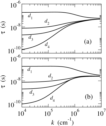
Figure 3: Relaxation time for an infinite iron thin film with thickness $d_{1}=1\times 10^{-6}$, $d_{2}=5\times 10^{-6}$, $d_{3}=1\times 10^{-5}$ and $d_{4}=5\times 10^{-5}$ cm for (a) configuration I and (b) configuration II.

The power dissipation clearly depends on $\omega$ which is a function of $k$. Owing to the strong influence of the magnetostatic energy within the magnon Hamiltonian, the derivation of this relationship is nontrivial, but, fortunately has been described by previous workers. Essentially, the Hamiltonian of the system has contribution from exchange, magnetostatic and Zeeman energy. We shall restrict ourselves to isotropic systems and therefore crystallographic anisotropy will have negligible effect to our result. We will only consider magnons with wavelength much greater than the lattice constant, e.g. $k\leq 10^{7}$ cm^-1 which applies to most magnons of interest. The dispersion relation for a thin film is given by S1970PRB

$$\omega=\gamma\sqrt{\left(H_{i}+\frac{2A}{M_{S}}k^{2}\right)\left(H_{i}+\frac{2A}{M_{S}}k^{2}+2\omega_{d}\right)}$$ (8)

where $H_{i}=H_{{\mathrm{ext}}}-NM_{S}$ is the internal field, $A$ is the exchange constant, $N$ is the demagnetizing factor and $H_{{\mathrm{ext}}}$ is the external magnetic field. The magnetostatic contribution is given by

$$\omega_{d}^{\mathrm{I}} = 2\pi M_{S}$$

$$\omega_{d}^{\mathrm{II}} = 2\pi M_{S}\left[\frac{1-e^{-kd}}{kd}\right]$$

The dispersion relation for an iron thin film of various thicknesses is shown in Fig. 2. Note that the curves converge for $k\gtrapprox 2\times 10^{6}$ cm^-1 where exchange interaction starts dominating the thickness dependent magnetostatic interaction.

The energy density of the system consists of the exchange, the magnetostatic and the Zeeman terms

$$\mathcal{E}(k,d)=A\left(\frac{\nabla M}{M_{S}}\right)^{2}+\mathcal{E}_{d}-\mathbf{M}\cdot\mathbf{H}_{\mathrm{ext}}$$ (10)

where the magnetostatic contribution to the energy is obtained by taking the negative scalar product of magnetization and the magnetic field produced by the magnons and is given by

$$\mathcal{E}_{d}^{\mathrm{I}} = 2\pi\epsilon^{2}$$

$$\mathcal{E}_{d}^{\mathrm{II}} = 2\pi\epsilon^{2}\left[\frac{1-e^{-kd}}{kd}\right]$$

Eqs. (LABEL:eq:power), (7), (8), (LABEL:eq:omegamag), (10) and (LABEL:eq:energymag) show that the energy decays exponentially with relaxation time:

$$\tau(k,d)=\frac{\mathcal{E}(k,d)}{P(k,d)}$$

This is the leading order term contributing to the relaxation time as the energy of the system gets renormalized by the magnetic field generated by the magnon-induced currents. Fig. 3 shows the relaxation time of spin waves in an iron thin film where the spin wave is confined in the $x-y$ plane. According to DV2003PRL the four magnon scattering produces magnons with wave vectors in the range $1-5\times 10^{6}$ cm^-1. It is important to note that magnetostatic is the dominant interaction in the long wavelength limit whereas exchange takes over in the short wavelength regime. The crossover, which happens around $k\sim 10^{6}$ cm^-1 in the range of thickness of the sample we are interested in, is of the same order of magnitude for bulk magnetic crystals Mills . This feature is nicely reproduced in our result where changing the value of the exchange constant only affects the curves for $k\geq 10^{6}$ cm^-1.

Both for configurations I and II, $\tau$ increases with $k$ for thicker films in the magnetostatic regime and saturates in the exchange regime. For such films the electric field and hence the power shows an inverse dependence with the wave vector in the long wavelength limit whereas the energy of the system is independent of $k$ in configuration I and changes slowly with $k$ in configuration II. This makes $\tau$ an increasing function of $k$ except for small thicknesses of the film in which case the power dissipation becomes nearly independent of $k$. However, both $\mathcal{E}$ and $P$ increases as $k^{2}$ in the exchange regime thereby making $\tau$ independent of $k$.

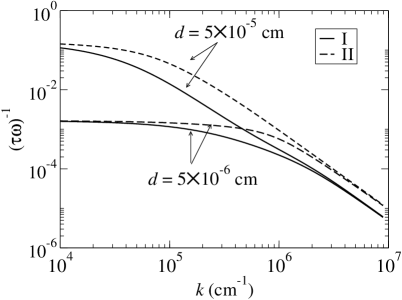
Figure 4: The quantity $1/\tau\omega$ as a function of the wave vector for two different thicknesses.

Fig. 4 shows the behavior of the quantity $1/\tau\omega$ as a function of the wave vector. This quantity, which can be interpreted as a wave vector dependent damping constant, is a measure of the amount of energy taken away from the system per precessional cycle. This damping constant should not be confused with the typical Gilbert damping constant used for uniform rotation of the element magnetization. However, the presence of values approaching $0.2$ illustrates the large magnitude of the effects described here.

Observation of spin wave resonance ST1958PRL in a thin film allows calculation of relaxation times from measured line widths. For example, analysis of Okochi’s O1970JPSJ data for his first spin wave resonance mode yields a damping constant $\alpha=0.0063$. Calculations for this configuration yield $P=32\pi^{2}\epsilon^{2}\omega^{2}\sigma/(c^{2}k^{2})$ and $\mathcal{E}=(2Ak^{2}/M^{2}_{S}-4\pi+H_{\mathrm{ext}}/M_{S})\epsilon^{2}$. The resulting value of the damping constant is $0.0095$ (using $A=10^{-6}$ erg/cm and $\sigma=2.9\times 10^{16}$ s^-1 PMW1966JAP for FeNi). The discrepancy is presumably due to conductivity differences between the two thin film samples. It is worth noting these experiments rely on exciting standing waves along the perpendicular direction of the thin film. This geometry typically minimizes the effect (relative to the configurations discussed elsewhere in this text) of magnon induced currents in the relaxation time because the magnon generated magnetic field is zero which makes the induced electric fields weaker and the rate of energy dissipation slower.

The effect of conductivity on the magnon-electron dissipation mechanism can be studied in magnetic semiconductors such as CdCr₂Se₄ and HgCr₂Se₄ whose conductivity can be tuned by the amount of Ag doping FC1978SSC ; FC1996PRB . The typical conductivity of such materials is several orders of magnitude lower than that of a ferromagnetic metal. For example, a 0.75 mole $\%$ Ag doped CdCr₂Se₄ has $\sigma=4.5\times 10^{11}$ s^-1 at $T=120$K. Therefore, the coefficient of expansion in Eq. (1) becomes much smaller compared to that for a ferromagnetic metal thereby making our formalism highly applicable for such materials. Assuming a resonance field $H_{\mathrm{res}}=3500$ Oe FC1996PRB and $\omega=\gamma H_{\mathrm{res}}$ we obtain a linewidth $\Delta H=1/(\tau\gamma)=78$ Oe for configuration I and $\Delta H=144$ Oe for configuration II, using $d=0.2$ mm and $k=1/d$. These values are in very good agreement with the FMR linewidths observed by Ferreira and Coutinho-Filho FC1978SSC . Under the experimental condition the exchange contribution to the energy is negligible and the magnetostatic and the Zeeman energies are of the same order of magnitude. In this limit, therefore, the magnon-electron contribution to the energy dissipation (calculated here) is comparable to that of conventional Eddy current loss obtained from the FMR linewidth by subtracting the effect of two magnon scattering Sparks1967IBID .

We conclude by proposing the following picture of ferromagnetic relaxation in switching experiments. We expect that the initial rapid approach of magnetization direction to equilibrium is enabled by magnon-magnon scattering that converts the energy into the higher spin wave modes. These modes then decay at a slower pace via the magnon-electron interaction described here or by the traditionally invoked mechanisms in less pure, lower conductivity films. This delay will lead to a small reduction in magnetization which appears to have been observed by Silva et al SKP2002APL .

This work was supported primarily by the MRSEC Program of the National Science Foundation under Award Number DMR-0212302. We thank Paul Crowell and Alexander Dobin for useful discussions.

References

- (1) W. K. Hiebert, A. Stankiewicz and M. R. Freeman, Phys. Rev. Lett. 79, 1134 (1997).
- (2) B. C. Choi, M. Belov, W. K. Hiebert, G. E. Ballentine, and M. R. Freeman, Phys. Rev. Lett. 86, 728 (2001).
- (3) Y. Acremann and C. H. Back, Science 290, 492 (2000).
- (4) A. Y. Dobin and R. H. Victora, Phys. Rev. Lett. 90, 167203 (2003).
- (5) E. Abrahams, Phys. Rev. 98, 387 (1955).
- (6) V. Kambersky and C. E. Patton, Phys. Rev. B. 11, 2668 (1975) and references therein.
- (7) N. S. Almeida and D. L. Mills, Phys. Rev. B. 53, 12232 (1996).
- (8) T. Holstein and H. Primakoff, Phys. Rev. 58, 1098 (1940).
- (9) J. D. Jackson, Classical Electrodynamics (John Wiley and Sons, New York, 1975).
- (10) T. Holstein and H. Primakoff, Phys. Rev. 58, 1098 (1940).
- (11) M. Sparks, Phys. Rev. B. 1, 3831 (1970).
- (12) D. L. Mills, Surface Excitations, Modern Problems in Condensed Matter Science Vol. 9, edited by V. M. Agranovich and R. Loudon (Elsevier, Amsterdam, 1984).
- (13) M. H. Seavey and P. E. Tannenwald, Phys. rev. Lett. 1, 168 (1958).
- (14) M. Okochi, J. Phys. Soc. Jap. 28, 897 (1970).
- (15) C. E. Patton, T. C. McGill and C. H. Wilts, J. App. Phys. 37, 3594 (1966).
- (16) J. M. Ferreira and M. D. Coutinho-Filho, Phys. Rev. B. 54, 12979 (1996).
- (17) J. M. Ferreira and M. D. Coutinho-Filho, Solid State Comm. 28, 775 (1978).
- (18) M. Sparks, J. Appl. Phys. 38, 1031 (1967).
- (19) T. J. Silva, P. Kabos and M. R. Pufall, Appl. Phys. Lett. 81, 2205 (2002).