An Exact SU(2) Symmetry and Persistent Spin Helix in a Spin-Orbit Coupled System

Abstract

Spin-orbit coupled systems generally break the spin rotation symmetry. However, for a model with equal Rashba and Dresselhauss coupling constant (the ReD model), and for the $[110]$ Dresselhauss model, a new type of $SU(2)$ spin rotation symmetry is discovered. This symmetry is robust against spin-independent disorder and interactions, and is generated by operators whose wavevector depends on the coupling strength. It renders the spin lifetime infinite at this wavevector, giving rise to a Persistent Spin Helix (PSH). We obtain the spin fluctuation dynamics at, and away, from the symmetry point, and suggest experiments to observe the PSH.

The physics of systems with spin-orbit coupling has generated great interest from both academic and practical perspectives S. A. Wolf et. al. (2001). In particular, spin-orbit coupling allows for purely electric manipulation of the electron spin J. Nitta et. al. (1997); Grundler (2000); Y. Kato et. al. (2004a, b), and could be of use in areas from spintronics to quantum computing. Theoretically, spin-orbit coupling reveals fundamental physics related to topological phases and their applications to the intrinsic and quantum spin Hall effectMurakami et al. (2003); J. Sinova et. al. (2004); C.L. Kane and E.J. Mele (2005); B.A. Bernevig and S.C. Zhang (2006); Qi et al. (a).

While strong spin-orbit interaction is useful for manipulating the electron spin by electric fields, it is also known to have the undesired effect of causing spin-decoherence M. I. Dyakonov et. al. (1986); Pikus and Titkov . The decay of spin polarization reflects the nonconservation of the total spin operator, $\vec{S}$, i.e. $[\vec{S},{\cal{H}}]\neq 0$, where ${\cal{H}}$ is any Hamiltonian that contains spin-orbit coupling. In this Letter, we identify an exact $SU(2)$ symmetry in a class of spin-orbit systems that renders the spin lifetime infinite. The symmetry involves components of spin at a finite wave vector, and is different from the $U(1)$ symmetry that has previously been associated with this class of models J. Schliemann et al. (2003); K.C. Hall et. al. (2003). As a result of this symmetry, spin polarization excited at a certain “magic” wavevector will persist. If this symmetry can be realized experimentally, it may be possible to manipulate spins through spin-orbit coupling without spin-polarization decay, at length scales characteristic of today’s semiconductor lithography.

We consider a two-dimensional electron gas without inversion symmetry, allowing spin-orbit coupling that is linear in the electron wavevector. The most general form of linear coupling includes both Rashba and Dresselhaus contributions:

$${\cal{H}}=\frac{k^{2}}{2m}+\alpha(k_{y}\sigma_{x}-k_{x}\sigma_{y})+\beta(k_{x}\sigma_{x}-k_{y}\sigma_{y}),$$ (1)

where $k_{x,y}$ is the electron momentum along the $[100]$ and $[010]$ directions respectively, $\alpha$, and $\beta$ are the strengths of the Rashba, and Dresselhauss spin-orbit couplings and $m$ is the effective electron mass. We shall be interested in the special case of $\alpha=\beta$, which may be experimentally accessible through tuning of the Rashba coupling via externally applied electric fields J. Nitta et. al. (1997). When $\alpha=\beta$, the spin-orbit coupling part of the Hamiltonian reads $\alpha(k_{x}+k_{y})(\sigma_{x}-\sigma_{y})$. Rotating the spatial coordinates by introducing $k_{\pm}=\frac{1}{\sqrt{2}}(k_{y}\pm k_{x})$, and also performing the global spin rotation generated by $U=\frac{1}{\sqrt{2}}(1+\frac{i}{\sqrt{2}}(\sigma_{x}+\sigma_{y}))$, brings the Hamiltonian to the diagonal form:

$${\cal{H_{\rm ReD}}}=U^{\dagger}{\cal{H}}U=\frac{k_{+}^{2}+k_{-}^{2}}{2m}-2\alpha k_{+}\sigma_{z}.$$ (2)

Throughout this paper, we shall be using both the original spin basis and the transformed spin basis for the $\cal{H_{\rm ReD}}$ model, depending on the context. It should always be remembered that $\sigma_{z}$ in the transformed spin basis corresponds to $\frac{1}{\sqrt{2}}(\sigma_{x}-\sigma_{y})$ in the original spin basis. $\cal{H_{\rm ReD}}$ is mathematically equivalent to the Dresselhauss $[110]$ model, describing quantum wells grown along the $[110]$ direction, whose Hamiltonian is given by:

$${\cal{H_{\rm[110]}}}=\frac{k_{x}^{2}+k_{y}^{2}}{2m}-2\alpha k_{x}\sigma_{z}.$$ (3)

As the Hamiltonians ${\cal{H_{\rm[ReD]}}}$ and ${\cal{H_{\rm[110]}}}$ are already diagonal, the energy bands (for ${\cal{H_{\rm[ReD]}}}$) are simply given by:

$$\epsilon_{\downarrow,\uparrow}(\vec{k})=\frac{k^{2}}{2m}\pm 2\alpha k_{+},$$ (4)

where $\downarrow,\uparrow$ are the spin components in the new, unitary transformed, spin basis: $\vec{S}\rightarrow U^{\dagger}\vec{S}U$. The bands in Eq.[4] have an important shifting property:

$$\epsilon_{\downarrow}(\vec{k})=\epsilon_{\uparrow}(\vec{k}+\vec{Q}),$$ (5)

where $Q_{+}=4m\alpha,Q_{-}=0$ for the ${\cal{H_{\rm[ReD]}}}$ model and $Q_{x}=4m\alpha,Q_{y}=0$ for the ${\cal{H_{\rm[110]}}}$ model. The Fermi surfaces consist of two circles shifted by the “magic” shifting vector $\vec{Q}$, as shown in Fig.[1].

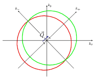
Figure 1: [Color Online] Fermi surfaces of the model consists of two circles shifted by the wavevector $\vec{Q}=(Q_{+},Q_{-})=(4m\alpha,0)$.

${\cal{H_{\rm[ReD]}}}$ and ${\cal{H_{\rm[110]}}}$ have the previously known $U(1)$ symmetry generated by $\sigma_{z}$ J. Schliemann et al. (2003); K.C. Hall et. al. (2003), which ensures long lifetime for uniform spin polarization along the z-axisY. Ohno et. al. (1999). The exact $SU(2)$ symmetry discovered in this work is generated by the following operators, expressed in the transformed spin basis as:

$$S^{-}_{Q}=\sum_{\vec{k}}c^{\dagger}_{\vec{k}\downarrow}c_{\vec{k}+\vec{Q}\uparrow},\;\;\;S^{+}_{Q}=\sum_{\vec{k}}c^{\dagger}_{\vec{k}+\vec{Q},\uparrow}c_{\vec{k}\downarrow}$$

$$S^{z}_{0}=\sum_{\vec{k}}c^{\dagger}_{\vec{k}\uparrow}c_{\vec{k}\uparrow}-c^{\dagger}_{\vec{k}\downarrow}c_{\vec{k}\downarrow},$$ (6)

with $c_{k\uparrow,\downarrow}$ being the annihilation operators of spin-up and down particles. These operators obey the commutation relations for angular momentum,

$$[S_{0}^{z},S^{\pm}_{Q}]=\pm 2S_{Q}^{\pm};\ \ [S^{+}_{Q},S^{-}_{Q}]=S_{0}^{z}$$ (7)

The shifting property Eq.[5] ensures that the operators defined in Eq.[6] commute with the Hamiltonian,

$$[{\cal{H_{\rm ReD}}},c^{\dagger}_{\vec{k}+\vec{Q}\uparrow}c_{\vec{k}\downarrow}]=(\epsilon_{\uparrow}(\vec{k}+\vec{Q})-\epsilon_{\downarrow}(\vec{k}))c^{\dagger}_{\vec{k}+\vec{Q}\uparrow}c_{\vec{k}\downarrow}=0$$ (8)

and similarly for $c^{\dagger}_{\vec{k}\downarrow}c_{\vec{k}+\vec{Q}\uparrow}$, thus uncovering the $SU(2)$ symmetry. This symmetry is robust against both spin-independent disorder and Coulomb (or other many-body) interactions as the spin operators commute with the finite-wave vector particle density $\rho_{q}=\sum_{k}c^{\dagger}_{\vec{k}+\vec{q}}c_{\vec{k}}$:

$$[\rho_{q},S_{Q}^{\pm}]=[\rho_{q},S^{z}_{0}]=0.$$ (9)

As a result single-particle potential scattering terms like $\sum_{q}V_{q}\rho_{q}$, as well as many-body interaction terms like $\sum_{q}V_{q}\rho_{q}^{\dagger}\rho_{q}$, all commute with the generators (6), and the $SU(2)$ symmetry is robust against these interactions.

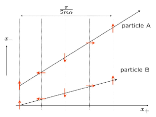
Figure 2: [Color Online] Spin configurations for two particles A and B depend only on the distance traveled along the $x_{+}$ axis and not on their initial momenta. For the same $x_{+}$ distance traveled, the spin precesses by exactly the same angle. After a length $L_{+}=2\pi\hbar/Q_{+}$ the spins all return exactly to the original configuration.

The $SU(2)$ conservation laws imply that the expectation values of $S^{z}$, $S_{Q}$, and $S_{Q}^{\dagger}$ have infinite lifetime. Since $S^{z}$ is a conserved quantity, a fluctuation of the $z$-component of spin polarization with wavevector $q$ can only decay by diffusion, which takes time $\tau_{s}=1/D_{s}q^{2}$, where $D_{s}$ is the spin diffusion constant. Notice that the hermitian operators $S_{x}(Q)=\frac{1}{2}(S_{Q}^{\dagger}+S_{Q})$ and $S_{y}(Q)=\frac{1}{2i}(S_{Q}^{\dagger}-S_{Q})$ create a helical spin density wave in which the direction of the spin polarization rotates in the $x,y$ plane in the transformed spin basis. Another manifestation of this symmetry is the vanishing of spin-dependent quantum interference (or weak anti-localization) at the $SU(2)$ point F.G. Pikus and G.E. Pikus (1995).

The infinite lifetime of the $S_{x},S_{y}$ spin helix with wave vector $\vec{Q}$ results from the combined effects of diffusion and precession in the spin-orbit effective field. A physical picture for the origin of the persistent spin helix (PSH) is sketched in Fig.[2], expressed in the transformed spin basis. Consider a particle propagating in the plane with momentum $\vec{k}$. In time $t$, it travels a distance along the $x_{+}$ direction $L_{+}=k_{+}t/m$, while its spin precesses about the $z$ axis by an angle $\theta=4\alpha k_{+}t/\hbar$. Eliminating $t$ from the latter equation yields $\theta=4\alpha mL_{+}/\hbar$, demonstrating that the net spin precession in the $x,y$ plane depends only on the net displacement in the $x_{+}$ direction and is independent of any other property of the electron’s path. Electrons starting with parallel spin orientation and the same value of $x_{+}$ will return exactly to the original orientation after propagating $L_{+}=2\pi\hbar/Q_{+}$.

For sake of clarity, we have depicted the PSH in Fig.[3] in the original basis. For a range of values in different materials from weak to strong spin-orbit splitting $\alpha=10^{2}\rightarrow 10^{4}(m/s)$, the characteristic wavelength of the PSH is $10\mu m\rightarrow 100nm$. In GaAs, the typical value is $L_{+}=1\mu m$. This characteristic wave length is on the scale of typical lithographic dimensions used in today’s semiconductor industry.

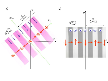
Figure 3: [Color Online] (a) PSH for the ${\cal{H_{\rm ReD}}}$ model. The spin-orbit magnetic field is in-plane (blue), whereas the spin helix, for the choice of the relative signs in Eq.[1] is in the $(x_{+},z)$ plane. (b) PSH for the ${\cal{H_{\rm[110]}}}$ model. The spin-orbit magnetic field $B^{spin}_{orbit}$, in blue, is out of plane, whereas the spin helix, in red, is in-plane.

Mathematically, the PSH is a direct manifestation of a “non-abelian” flux in the ground state of the ${\cal{H_{\rm ReD}}}$ and the ${\cal{H_{\rm[110]}}}$ models. Following Ref. (Jin et al., 2006), we express ${\cal{H_{\rm ReD}}}$ in the form of a background non-abelian gauge potential,

$${\cal{H_{\rm ReD}}}=\frac{k_{-}^{2}}{2m}+\frac{1}{2m}(k_{+}-2m\alpha\sigma_{z})^{2}+const.$$ (10)

In contrast to the general case where the non-abelian gauge potential leads to a finite non-abelian field strength, the field strength vanishes identically for $\alpha=\beta$. Therefore, we can eliminate the vector potential by a non-abelian gauge transformation: $\Psi_{\uparrow}(x_{+},x_{-})\rightarrow\exp(i2m\alpha x_{+})\Psi_{\uparrow}(x_{+},x_{-})$, $\Psi_{\downarrow}(x_{+},x_{-})\rightarrow\exp(-i2m\alpha x_{+})\Psi_{\downarrow}(x_{+},x_{-})$. Under this transformation, the spin-orbit coupled Hamiltonian is mapped to that of the free Fermi gas. The cost of the transformation is two-fold. First, the new wave function $\Psi(x_{+},x_{-})$ satisfies twisted spin boundary conditionsQi et al. (b). However, these have no physical effect, since a metallic system without off-diagonal-long-range-order is insensitive to a change of boundary conditions in the thermodynamic limit. Second, while diagonal operators such as the charge $n$ and $S_{z}$ remain unchanged, off-diagonal operators, such as $S^{-}(\vec{x})=\psi_{\downarrow}^{\dagger}(\vec{x})\psi_{\uparrow}(\vec{x})$ and $S^{+}(\vec{x})=\psi_{\uparrow}^{\dagger}(\vec{x})\psi_{\downarrow}(\vec{x})$ are transformed: $S^{-}(\vec{x})\rightarrow\exp(-i4m\alpha x_{+})S^{-}(\vec{x})$, $S^{+}(\vec{x})\rightarrow\exp(i4m\alpha x_{+})S^{+}(\vec{x})$. In the transformed basis, all three components of the spin obey the simple diffusion equation, as the Hamiltonian is just that for free electrons without spin-orbit coupling. Hence $S_{x}=const$ is a solution to the diffusion equation. Transforming back demonstrates that this solution corresponds to $(S_{x},S_{y})=(\cos(4m\alpha x_{+}),\sin(4m\alpha x_{+}))=const$ ., which is the PSH.

While spin is conserved at the $SU(2)$ point, dynamics emerge when the conditions $\vec{q}=\vec{Q}$ and/or $\alpha=\beta$ are not met. Solving for the coupled charge and spin dynamics requires Boltzman transport equations, which we obtain below using the Keyldish formalism Rammer and Smith (1986); E.G. Mishchenko et al. (2004). Assuming isotropic scattering with momentum lifetime $\tau$, the retarded and advanced Green’s functions are:

$$G^{R,A}(k,\epsilon)=(\epsilon-{\cal{H}}\pm\frac{i}{2\tau})^{-1}.$$ (11)

We introduce a momentum, energy, and position dependent charge-spin density which is a $2\times 2$ matrix $g(k,r,t)$. Summing over momentum:

$$\rho({r,t})\equiv\int\frac{d^{2}k}{(2\pi)^{3}\nu}g({k,r,t}),$$ (12)

gives the real-space spin-charge density $\rho(r,t)=n(r,t)+S^{i}(r,t)\sigma_{i}$, where $n(r,t)$ and $S^{i}(r,t)$ are the charge and spin density and $\nu={m}/{2\pi}$ is the density of states in two-dimensions. $\rho(r,t)$ and $g(k,r,t)$ satisfy a Boltzman-type equation Rammer and Smith (1986); E.G. Mishchenko et al. (2004):

$$\frac{\partial g}{\partial t}+\frac{1}{2}\left\{\frac{\partial{\cal{H}}}{\partial k_{i}},\frac{\partial g}{\partial r_{i}}\right\}+i\left[{\cal{H}},g\right]=-\frac{g}{\tau}+\frac{i}{\tau}(G^{R}\rho-\rho G^{A}).$$ (13)

that we now solve for the Hamiltonian of Eq.[1] for arbitrary $\alpha,\beta$. To obtain the spin-charge transport equations, we follow the sequence: time-Fourier transform the above equation; find a general solution for $g(k,r,t)$ involving $\rho(r,t)$ and the $k$-dependent spin-orbit coupling; perform a gradient expansion of that solution (assuming $\partial_{r}<<k_{F}$ where $k_{F}$ is the Fermi wavevector) to second order; and, finally, integrate over the momentum. The anisotropic nature of the Fermi surfaces when both $\alpha$ and $\beta$ are nonzero introduces coupling of charge and spin degrees of freedom beyond what was found with only Rashba coupling Burkov et al. (2004). The final result, expressed in the $i=(x_{+},x_{-},z)$ spatial coordinates and the original spin basis, is:

$$\partial_{t}n=D\partial_{i}^{2}n+B_{1}\partial_{x_{+}}S_{x_{-}}-B_{2}\partial_{x_{-}}S_{x_{+}}$$ (14)

$$\partial_{t}S_{x_{-}}=D\partial_{i}^{2}S_{x_{-}}+B_{1}\partial_{x_{+}}n-C_{2}\partial_{x_{-}}S_{z}-T_{2}S_{x_{-}}$$ (15)

$$\partial_{t}S_{x_{+}}=D\partial_{i}^{2}S_{x_{+}}-B_{2}\partial_{x_{-}}n-C_{1}\partial_{x_{+}}S_{z}-T_{1}S_{x_{+}}$$ (16)

$$\partial_{t}S_{z}=D\partial_{i}^{2}S_{z}+C_{2}\partial_{x_{-}}S_{x_{-}}+C_{1}\partial_{x_{+}}S_{x_{+}}-(T_{1}+T_{2})S_{z}.$$ (17)

With an effective $k_{F}$ defined as $\sqrt{2mE_{F}}$, the constants in the above equations are:

$$B_{1}=2(\alpha-\beta)^{2}(\alpha+\beta)k_{F}^{2}\tau^{2},$$

$$B_{2}=2(\alpha+\beta)^{2}(\alpha-\beta)k_{F}^{2}\tau^{2},$$

$$C_{1}=2\frac{1}{m}(\alpha+\beta)k_{F}^{2}\tau,\;\;\;\;C_{2}=2\frac{1}{m}(\alpha-\beta)k_{F}^{2}\tau$$

$$T_{1}=2(\alpha+\beta)^{2}k_{F}^{2}\tau,\;\;\;\;T_{2}=2(\alpha-\beta)^{2}k_{F}^{2}\tau.$$ (18)

The diffusion constant $D=v_{F}^{2}\tau/2$. Our results for the coupling coefficients are valid in the diffusive limit $\alpha k_{F}\tau<<1,\;\beta k_{F}\tau<<1$ and reduce to the appropriate limits in the cases $\beta\rightarrow 0$ or $\alpha\rightarrow 0$ Burkov et al. (2004); E.G. Mishchenko et al. (2004). We observe that for a general direction of propagation in the $x_{\pm}$ plane, the three components of spin, and the charge, are all coupled.

Motivated by experiments that probe spin dynamics optically, we focus on the behavior of the out-of-plane component of the spin, which is $S_{z}$ in the original basis. We assume a space-time dependence proportional to $\exp[i(\omega t-\vec{q}\cdot\vec{r})]$, and compare $\vec{q}$ parallel to $[1\bar{1}0]$ and $\vec{q}$ parallel to $[110]$.

The spin polarization lifetime for $\vec{q}$ parallel to $[1\bar{1}0]$ is not enhanced, as no shifting property exists in this direction. For this orientation, the four equations [14-17] separate into two coupled pairs, with $n$ being coupled to $S_{x_{+}}$ and $S_{z}$ coupled to $S_{x_{-}}$. The optical probe will detect the characteristic frequencies that are solutions to the equation that couples $S_{z}$ with $S_{x_{-}}$:

$$i\omega_{1,2}=-Dq^{2}-\frac{1}{2}(2T_{2}+T_{1}\pm\sqrt{T_{1}^{2}+4q^{2}C_{2}^{2}}).$$ (19)

At $\alpha=\beta$ we have $T_{2}=C_{2}=0$ and the characteristic frequencies become $i\omega_{1}=-Dq^{2}-T_{1}$, $i\omega_{2}=-Dq^{2}$.

The spin polarization dynamics are qualitatively different in the $[110]$ direction, which is the direction along which the Fermi surfaces are shifted. In this case the four equations again decouple into two pairs, with $n$ coupled to $S_{x_{-}}$ and $S_{z}$ coupled to $S_{x_{+}}$. The characteristic frequencies are:

$$i\omega_{1,2}=-Dq^{2}-\frac{1}{2}(2T_{1}+T_{2}\pm\sqrt{T_{2}^{2}+4q^{2}C_{1}^{2}}).$$ (20)

We note that $i\omega_{2}(q)$ has a minimum at a wavevector that depends only on $\alpha,\beta$, and $m$, $i.e.$, is independent of $k_{F}$ and $\tau$. When $\alpha=\beta$ the decay rates become $i\omega_{1,2}=-Dq^{2}-T_{1}\mp C_{1}q$, and $i\omega_{2}(q)$ is zero (corresponding to the PSH) at the shifting wave-vector $4m\alpha$. We have checked that this relation continues to hold as we include higher order corrections to the transport coefficients. Earlier calculations based on the pure Rashba model V.A. Froltsov (2001); Burkov et al. (2004) also predict an increased spin lifetime at a finite wave vector $(\sqrt{15}/{2})\alpha m$, but the lifetime is enhanced relative to $q=0$ only by the factor $16/7$.

Transient spin-grating experiments A.R. Cameron et al. (1996); C.P. Weber et. al (2005) are particularly well-suited to testing our theoretical predictions (Eqs.[19,20]) and discovering the PSH, as they inject finite wavevector spin distributions. If at $t=0$ an $S_{z}$ polarization proportional to $\cos(qx_{+})$ is excited, we predict a time evolution,

$$S_{z}(q,t)=A_{1}(q)e^{i\omega_{1}(q)t}+A_{2}(q)e^{i\omega_{2}(q)t},$$ (21)

where

$$A_{1,2}(q)=\frac{1}{2}\left[1\pm\frac{T_{2}}{\sqrt{T_{2}^{2}+4q^{2}C_{1}^{2}}}\right].$$ (22)

Thus, according to theory, the photoinjected spin polarization wave will decay as a double exponential, with characteristic decay rates $i\omega_{1,2}(q)$. As $\alpha\rightarrow\beta$ the weight factors of the two exponentials become equal and the decay rate of the slower component $\rightarrow 0$ at the “magic” wave-vector. If transient grating measurements verify these predictions, they will be able to provide rapid and accurate determination of the spin-orbit Hamiltonian, enabling tuning of sample parameters to achieve $\alpha=\beta$.

In conclusion, we have discovered a new type of spin $SU(2)$ symmetry in a class of spin-orbit coupled models including the ReD model and the Dresselhauss $[110]$ model. Based on this symmetry, we predict the existence of a Persistent Spin Helix. The lifetime of the PSH is infinite within these models, but of course there will be other relaxation mechanisms which would lead to its eventual decay. We obtained the transport equations for arbitrary strength of Rashba and Dresselhauss couplings and these equations provide the basis to analyze experiments in search of the PSH.

B.A.B. wishes to acknowledge the hospitality of the Kavli Institute for Theoretical Physics at University of California at Santa Barbara, where part of this work was performed. This work is supported by the NSF through the grants DMR-0342832, by the US Department of Energy, Office of Basic Energy Sciences under contract DE-AC03-76SF00515, the Western Institute of Nano-electronics and the IBM Stanford SpinApps Center.

References

- S. A. Wolf et. al. (2001) S. A. Wolf et. al., Science 294, 1488 (2001).
- J. Nitta et. al. (1997) J. Nitta et. al., Phys. Rev. Lett. 78, 1335 (1997).
- Grundler (2000) D. Grundler, Phys. Rev. Lett. 84, 6074 (2000).
- Y. Kato et. al. (2004a) Y. Kato et. al., Phys. Rev. Lett. 93, 176601 (2004a).
- Y. Kato et. al. (2004b) Y. Kato et. al., Nature 427, 50 (2004b).
- Murakami et al. (2003) S. Murakami, N. Nagaosa, and S. Zhang, Science 301, 1348 (2003).
- J. Sinova et. al. (2004) J. Sinova et. al., Phys. Rev. Lett. 92, 126603 (2004).
- C.L. Kane and E.J. Mele (2005) C.L. Kane and E.J. Mele, Phys. Rev. Lett. 95, 226801 (2005).
- B.A. Bernevig and S.C. Zhang (2006) B.A. Bernevig and S.C. Zhang, Phys. Rev. Lett. 96, 106802 (2006).
- Qi et al. (a) X. Qi, Y. Wu, and S. Zhang, cond-mat/0505308.
- M. I. Dyakonov et. al. (1986) M. I. Dyakonov et. al., Sov. Phys. JETP 63, 655 (1986).
- (12) G. Pikus and A. Titkov, Optical Orientation (North-Holland, Amsterdam, 1984).
- J. Schliemann et al. (2003) J. Schliemann, J.C. Egues, and D. Loss, Phys. Rev. Lett. 90, 146801 (2003).
- K.C. Hall et. al. (2003) K.C. Hall et. al., Appl. Phys. Lett 83, 2937 (2003).
- Y. Ohno et. al. (1999) Y. Ohno et. al., Phys. Rev. B 83, 4196 (1999).
- F.G. Pikus and G.E. Pikus (1995) F.G. Pikus and G.E. Pikus, Phys. Rev. B 51, 16928 (1995).
- Jin et al. (2006) P. Q. Jin, Y. Q. Li, and F. C. Zhang, J. Phys. A 39, 7115 (2006).
- Qi et al. (b) X. Qi, Y. Wu, and S. Zhang, cond-mat/0604071.
- Rammer and Smith (1986) J. Rammer and H. Smith, Rev. Mod. Phys. 58, 323 (1986).
- E.G. Mishchenko et al. (2004) E.G. Mishchenko, A.V.Shytov, and B.I. Halperin, Phys. Rev. Lett. 93, 226602 (2004).
- Burkov et al. (2004) A. Burkov, A. Nunez, and A. MacDonald, Phys. Rev. B 70, 155308 (2004).
- V.A. Froltsov (2001) V.A. Froltsov, Phys. Rev. B 64, 045311 (2001).
- A.R. Cameron et al. (1996) A.R. Cameron, P. Riblet, and A. Miller, Phys. Rev. Lett. 76, 4793 (1996).
- C.P. Weber et. al (2005) C.P. Weber et. al, Nature 437, 1330 (2005).