Scaling relations in the quasi-two-dimensional Heisenberg antiferromagnet

Abstract

The large-$N$ expansion of the quasi-two-dimensional quantum nonlinear $\sigma$ model is used in order to establish experimentally applicable universal scaling relations for the quasi-two-dimensional Heisenberg antiferromagnet. We show that, at $N=\infty$, the renormalized coordination number introduced by Yasuda et al. [Phys. Rev. Lett. 94, 217201 (2005)] is a universal number in the limit of $J^{\prime}/J\rightarrow 0$. Moreover, similar scaling relations proposed by Hastings and Mudry [Phys. Rev. Lett. 96, 027215 (2006)] are derived at $N=\infty$ for the three-dimensional static spin susceptibility at the wave vector $(\pi,\pi,0)$, as well as for the instantaneous structure factor at the same wave vector. We then use $1/N$ corrections to study the relation between interplane coupling, correlation length, and critical temperature, and show that the universal scaling relations lead to logarithmic corrections to previous mean-field results.

I Introduction

Many materials, such as copper oxides and other layered perovskites, are known to be nearly two-dimensional magnets. While in certain intermediate temperature ranges these systems are well described by purely two-dimensional models, three dimensionality is restored at temperatures below an energy scale that is governed by the ratio between the interlayer coupling $J^{\prime}$ and the intraplanar exchange parameter $J$. For example, two-dimensional quantum Heisenberg antiferromagnets (AFs) do not support long-range collinear magnetic order at any finite temperature according to the Mermin-Wagner theorem,Mermin-Wagner while real layered systems, such as La${}^{\ }_{2}$CuO${}^{\ }_{4}$, do. The anisotropy $J^{\prime}/J$ of a quasi-two-dimensional material can be determined from the spin-wave dispersion below the ordering temperature. It can also be determined from the measured ordering temperature provided one understands the two-dimensional to three-dimensional crossover that manifests itself in the dependence on $J^{\prime}/J$ of the ordering temperature.

A common approximation for the ordering temperature $T^{\ }_{\mathrm{c}}$ of a quasi-$n$-dimensional magnetic system is the random-phase approximation (RPA), Scalapino ; Schultz96 which predicts that

$$J^{\prime}\chi^{(n)}_{\mathrm{c}}=\frac{1}{z^{(n)}}.$$ (1)

Here $\chi^{(n)}_{\mathrm{c}}$ is the exact static susceptibility associated to the magnetic order for the underlying $n$-dimensional subsystem evaluated at the ordering temperature $T^{\ }_{\mathrm{c}}$ and $z^{(n)}$ is the coordination number of the $n$-dimensional subsystem. Yasuda et al. in Ref. Yasuda05, have quantified the accuracy of the RPA in two steps. First, they computed the three-dimensional AF ordering temperature $T^{\ }_{AF}$ with the help of a quantum (classical) Monte Carlo (MC) simulation of a spin-$S$ ($S=\infty$ in the classical system) nearest-neighbor Heisenberg model on a cubic lattice with AF exchange coupling $J^{\prime}$ along the vertical axis and AF exchange coupling $J$ within each layer of the cubic lattice. Second, they computed the two-dimensional static staggered susceptibility $\chi^{(2)}_{s}$ evaluated at $T^{\ }_{AF}$ from step 1 after switching off $J^{\prime}$. They thus showed that, for small $J^{\prime}/J$, $T^{\ }_{AF}$ is given by a modified random-phase approximation, in which the coordination number gets renormalized,

$$z^{(2)}\longrightarrow\zeta^{(2)}.$$ (2)

It turns out that the renormalization $\zeta^{(2)}$ of the coordination number $z^{(2)}=2$ converges as $J^{\prime}/J\to 0$ to a value that is independent of the spin quantum number $S$ taking values in $1/2,1,\dots,\infty$. This fact motivated them to conjecture the universality of the effective coordination number $\zeta^{(2)}$ in the limit $J^{\prime}/J\rightarrow 0$.

The results of Yasuda et al. were shown by Hastings and Mudry in Ref. Hastings06, to reflect the so-called renormalized classical (RC) regime of the underlying two-dimensional subsystem. Hastings and Mudry predicted that if the two-dimensional subsystem is characterized by a quantum critical (QC) regime, then the effective coordination number in the limit $J^{\prime}/J\rightarrow 0$ is a universal function of the ratio $c\beta^{\ }_{AF}/\xi^{(2)}$ – a number of order 1 in the QC regime as opposed to a vanishing number in the RC regime – where $c$ is the two-dimensional spin-wave velocity, $\beta^{\ }_{AF}=1/T^{\ }_{AF}$, and $\xi^{(2)}$ is the two-dimensional correlation length.

Hastings and Mudry also proposed universal scaling relations involving observables of the quasi-two-dimensional system only. One of these scaling relations is obtained from multiplying the static three-dimensional spin susceptibility $\chi^{(3)}_{s}$ evaluated at the wave vector $(\pi,\pi,0)$ and at the Néel temperature with $J^{\prime}$. Another scaling relation can be derived by multiplying the instantaneous structure factor at the transition temperature $S^{(3)}(\pi,\pi,0;t=0;T^{\ }_{AF})$ with $J^{\prime}$ and the inverse Néel temperature $1/T^{\ }_{AF}$. This last universal relation has the advantage of being directly measurable with the help of inelastic neutron scattering.

The aim of this work is to verify the universal scaling laws proposed above within the $N=\infty$ approximation to the quasi-two-dimensional quantum nonlinear $\sigma$ model (QNLSM). Our starting point is the two-dimensional QNLSM (a two-space and one-time NLSM), which is believed to capture the physics of two-dimensional quantum Heisenberg AF at low energies. Chakravarty88 ; Chakravarty89 ; Chubukov94 Assuming that the physics of a single layer can be approximated by the two-dimensional QNLSM, we introduce the interlayer coupling following Refs. Chakravarty88, , Chakravarty89, , Affleck96, , and Irkhin97, . We then show that, in the $N=\infty$ approximation, the quantities $J^{\prime}\chi^{(2)}_{s}(T^{\ }_{AF})$, $J^{\prime}\chi^{(3)}(\pi,\pi,0;\omega=0,T^{\ }_{AF})$, and $J^{\prime}S^{(3)}(\pi,\pi,0;t=0;T^{\ }_{AF})/T^{\ }_{AF}$ each converge to universal scaling functions of the dimensionless ratio between the thermal de Broglie wavelength of spin waves and a correlation length in the limit $J^{\prime}/J\to 0$. As in the strict two-dimensional limit, different regimes can be distinguished depending on the value taken by this dimensionless ratio. The form of the nonuniversal corrections to the universal functions obtained in the limit $J^{\prime}/J\rightarrow 0$ strongly depends on these regimes. In the renormalized classical (RC) regime, which is dominated by classical thermal fluctuations, the nonuniversal corrections are relatively small for small $J^{\prime}/J$, as is seen from MC simulations. Yasuda05 Near the critical coupling of the two-dimensional QNLSM, fluctuation physics is predominantly quantum. In this quantum regime, the universal constants obtained in the limit $J^{\prime}/J\rightarrow 0$ depend on the way this limit is taken, i.e., on the value taken by the fixed ratio (24) between the characteristic length scale of the quantum fluctuations and the characteristic length scale at which interplane interactions become important. When this ratio is a large number, the fluctuation regime is the quantum critical (QC) regime. When this ratio is of order 1, the fluctuation regime is the quantum disordered (QD) regime. When this ratio is much smaller than 1, the quasi-two-dimensional system remains disordered all the way down to zero temperature.

The universal relations described above have recently been tested numerically by Yao and Sandvik. Yao06 They have performed quantum Monte-Carlo simulations of spin-$1/2$ quasi-two-dimensional systems in the RC, QC, and QD regimes. Their results qualitatively agree with the predictions of the large-$N$ expansion proposed here.

We state the universal scaling laws in Sec. II. The quasi-two-dimensional QNLSM, which is the basis of our analysis, is defined in Sec. III. The $N=\infty$ approximation to the Néel temperature is given in Sec. IV. Scaling laws in the $N=\infty$ approximation are derived for the quasi-two-dimensional QNLSM in Sec. V and for its classical limit, the quasi-two-dimensional NLSM, in Sec. VI. Conclusions are presented in Sec. VIII while we defer to the appendixes for the derivation of the counterparts to these scaling laws in the case of the quasi-one-dimensional Ising model. Among the most important conclusions is an extension to finite $N$, where we relate $J^{\prime},\,J,\,T_{AF},\,\xi^{(2d)}$ and find scaling relations that differ from mean-field estimates by logarithmic corrections.

II Universal scaling relations

We are going to formulate precisely the universal relations discussed in Sec. I. It is instructive and necessary to first identify the relevant length scales of the system near the crossover between two dimensionality and three dimensionality. These will be used to construct the relevant dimensionless scaling variables whose values will allow us, in turn, to separate different scaling regimes.

II.1 Characteristic length scales

We start with the Hamiltonian describing a spatially anisotropic Heisenberg AF on a cubic lattice,

$$H:=J\sum_{\langle ii^{\prime}\rangle}\sum_{j}\boldsymbol{S}^{\ }_{i,j}\cdot\boldsymbol{S}^{\ }_{i^{\prime},j}+J^{\prime}\sum_{i}\sum_{\langle jj^{\prime}\rangle}\boldsymbol{S}^{\ }_{i,j}\cdot\boldsymbol{S}^{\ }_{i,j^{\prime}}.$$ (3)

Planar coordinates of the cubic lattice sites are denoted by the letters $i$ and $i^{\prime}$. The letters $j$ and $j^{\prime}$ label each plane. The angular bracket $\langle ii^{\prime}\rangle$ denotes planar nearest-neighbor sites. The angular bracket $\langle jj^{\prime}\rangle$ denotes two consecutive planes. A spin operator located at site $i$ in the $j$th plane is denoted by $\boldsymbol{S}^{\ }_{i,j}$. It carries the spin quantum number $S=1/2,1,\dots$ . The coupling constants are AF, $J,\,J^{\prime}>0$, and are strongly anisotropic, $J\gg J^{\prime}$.

We are interested in the thermodynamic properties of the system at the AF ordering temperature $T^{\ }_{AF}$. At this temperature, there exists a diverging length scale, the temperature-dependent correlation length

$$\xi\equiv\xi^{(3)}_{\pi,\pi,\pi},$$ (4)

for AF correlations at the wave vector $(\pi,\pi,\pi)$. For a quasi-two-dimensional AF, the strong spatial anisotropy $J\gg J^{\prime}>0$ allows us to identify the characteristic length scale

$$\xi^{\prime}:=\sqrt{\frac{1}{\mathcal{Z}^{\prime}}}\sqrt{\frac{J}{J^{\prime}}}\ a,$$ (5a)

where $$a \mathcal{Z}^{\prime} N=\infty \left.\mathcal{Z}^{\prime}\right|^{\ }_{N=\infty}=1 1/N$$ is the lattice spacing of the cubic lattice and is a multiplicative renormalization.footnote: Z' In the approximation considered in this paper, . We will omit this renormalization factor in the following until we treat corrections in Sec. VII.1.

In a good quasi-two-dimensional Heisenberg AF

$$0<J^{\prime}\ll J\Longrightarrow\xi^{\prime}\gg a.$$ (5b)

It was proposed Affleck96 ; Irkhin97 that $\xi^{\prime}$ determines the crossover between two and three dimensionality. Heuristically, the temperature dependence of the AF correlation length is nothing but that of the two-dimensional underlying system $\xi^{(2)}$ as long as $\xi^{(2)}\ll\xi^{\prime}$. Upon approaching $T^{\ }_{AF}$ from above, $\xi^{(2)}$ grows until $\xi^{(2)}\sim\xi^{\prime}$. Below this temperature, three-dimensionality is effectively recovered and AF long-range order becomes possible.

In the regime of temperature above the ordering temperature $T^{\ }_{AF}$ for which $\xi^{(2)}\gg a$, the two-dimensional spin-wave velocity $c$ is well defined and depends weakly on temperature. Together with the inverse Néel temperature $\beta^{\ }_{AF}$, we can then build the thermal de Broglie wavelength $c\beta^{\ }_{AF}$. Equipped with the characteristic length scales $c\beta^{\ }_{AF}$ and $\xi^{\prime}$, we can define three regimes. (i) The renormalized classical (RC) regime is defined by the condition

$$a\ll c\beta^{\ }_{AF}\ll\xi^{\prime}.$$ (6)

(ii) The quantum critical (QC) regime is defined by the condition

$$a\ll c\beta^{\ }_{AF}\simeq\xi^{\prime}.$$ (7)

(iii) The quantum disordered (QD) regime is defined by the condition

$$a\ll\xi^{\prime}\ll c\beta^{\ }_{AF}.$$ (8)

In the first regime (6), fluctuations are predominantly two-dimensional and thermal. The planar correlation length diverges exponentially fast with decreasing temperature. This leads to a rather sharp crossover between two- and three-dimensionality. As a corollary, there will be small nonuniversal corrections to universality for finite $J^{\prime}/J$. In the second, Eq. (7), and third, Eq. (8), regimes, fluctuations are predominantly two-dimensional and quantum. In the QC regime (7), the underlying two-dimensional fluctuations are quantum critical. In the QD regime (8), they are quantum disordered.

Common to all three regimes (6)-(8) is the fact that the lattice spacing is much smaller than the de Broglie wavelength constructed from the two-dimensional spin-wave velocity and the three-dimensional ordering temperature. It is then reasonable to expect that planar fluctuations of the microscopic Hamiltonian (3) can be captured by an effective low-energy and long-wavelength effective continuum theory. We choose this effective field theory to be the two-dimensional QNLSM. Chakravarty88 ; Chakravarty89 ; Chubukov94 To account for interplanar fluctuations, we preserve the lattice structure by coupling in a discrete fashion an infinite array of two-space and one-time QNLSM. We shall call this effective theory the quasi-two-dimensional QNLSM. The ratio $c\beta^{\ }_{AF}/\xi^{\prime}$ is then determined by the parameters of the quasi-two-dimensional QNLSM, i.e., by the two-dimensional spin-wave velocity $c$ and spin stiffness $\rho^{\ }_{s}$ (or the gap $\Delta$), as well as on $J^{\prime}/J$. These are related to the microscopic parameters of the quantum Heisenberg AF. While the model with nearest-neighbor couplings and with physical spins ($S\geq 1/2$) is known to be in the RC regime at low temperatures, the addition of terms in the Hamiltonian (3) such as frustrating next-nearest-neighbor couplings, say, allows us to realize the QC or QD regimes. We thus consider the two-dimensional spin-wave velocity $c$ and spin stiffness $\rho^{\ }_{s}$ (or the gap $\Delta$) as phenomenological parameters.

The scaling functions we are looking for will depend on the ratios of the lengths $\xi^{\prime}$, $c\beta_{AF}$, and, if we are interested in an observable of the two-dimensional underlying system, of $\xi^{(2)}(\beta_{AF})$. However, at the transition temperature and in the limit of $J^{\prime}/J\to 0$, only one of the two ratios is independent, and the scaling functions will indeed depend only on one dimensionless parameter.Hastings06

II.2 Universal scaling functions

The first universal scaling function, suggested in Ref. Hastings06, , involves the two-dimensional static and staggered spin susceptibility,

$$\lim_{J^{\prime}/J\to 0}J^{\prime}\chi^{(2)}_{s}(\beta^{\ }_{AF})=F^{\ }_{1}\big{(}c\beta^{\ }_{AF}/\xi^{(2)}(\beta^{\ }_{AF})\big{)},$$ (9a)

where

$$\chi^{(2)}_{s}(\beta^{\ }_{AF}):=\chi^{(2)}(\boldsymbol{k}^{\ }_{AF},\omega=0;\beta^{\ }_{AF})$$ (9b)

with $\boldsymbol{k}^{\ }_{AF}=(\pi,\pi)$. In the RC regime,

$$F^{\ }_{1}\big{(}c\beta^{\ }_{AF}/\xi^{(2)}(\beta^{\ }_{AF})\big{)}=F^{\ }_{1}(0)\equiv 1/\zeta^{(2)}.$$ (10)

MC simulations give $\zeta^{(2)}\simeq 1.3$, Yasuda05 while the RPA approximation leads to $\zeta^{(2)}=2$. Using the $N=\infty$ approximation to the quasi-two-dimensional QNLSM, we will find $\zeta^{(2)}=1$ in the RC regime.

The two-dimensional spin-susceptibility is inaccessible experimentally at the three-dimensional ordering temperature. In order to mimic the two-dimensional AF wave vector in the three-dimensional system, we choose to work at the wave vector $(\pi,\pi,0)$. We claim the existence of the universal scaling function

$$\lim_{J^{\prime}/J\to 0}J^{\prime}\chi^{(3)}_{s}\big{(}\beta^{\ }_{AF}\big{)}=F^{\ }_{2}\big{(}c\beta^{\ }_{AF}/\xi^{\prime}\big{)},$$ (11a)

where we have defined

$$\chi^{(3)}_{s}\big{(}\beta^{\ }_{AF}\big{)}:=\chi^{(3)}\big{(}\pi,\pi,0,\omega=0;\beta^{\ }_{AF}\big{)}.$$ (11b)

Observe that any vector of the form $(\pi,\pi,k^{\ }_{z})$ with $k^{\ }_{z}\neq\pi$ would lead to the same conclusion but for different universal scaling functions that depend on $k^{\ }_{z}$. In the $N=\infty$ approximation of the quasi-two-dimensional QNLSM, we find that $F^{\ }_{2}(x)=1/4$ takes the same value in the RC, QC, and QD regimes. This suggests that this scaling relation is rather robust and well suited for numerical studies.

Finally, we claim the existence of the universal scaling function

$$\lim_{J^{\prime}/J\to 0}\beta^{\ }_{AF}J^{\prime}S^{(3)}\big{(}\pi,\pi,0,t=0;\beta^{\ }_{AF}\big{)}=F^{\ }_{3}\big{(}c\beta^{\ }_{AF}/\xi^{\prime}\big{)},$$ (12a)

where $$S^{(3)}$$ is the instantaneous structure factor

$$S^{(3)}(\boldsymbol{q},q_{z},t=0;\beta):=-\int_{-\infty}^{+\infty}\frac{d\omega}{\pi}\frac{\operatorname{Im}\,\chi^{(3)}(\boldsymbol{q},q_{z},\omega;\beta)}{e^{\beta\omega}-1}.$$ (12b)

In the $N=\infty$ approximation of the quasi-two-dimensional QNLSM, we find that $F^{\ }_{3}(x)=(x/4)\coth x$.

The reminder of the paper is devoted to proving the existence of these three universal scaling functions and to their computation in the $N=\infty$ approximation of the quasi-two-dimensional QNLSM.

III Quasi-two-dimensional QNLSM

The quantum nonlinear $\sigma$ model (QNLSM) was successfully used to study the low-energy and long-wavelength physics of the quantum one-dimensional Heisenberg AF, Haldane83 the quantum two-dimensional Heisenberg model AF, Chakravarty88 ; Chakravarty89 ; Chubukov94 and the quantum quasi-two-dimensional Heisenberg AF. Affleck96 ; Irkhin97 In Haldane’s mapping of the quantum Heisenberg AF to the QNLSM, Haldane83 a crucial role is played by the correlation length. A large correlation length gives the possibility to separate slow from fast modes. Integration over fast modes can then be carried out perturbatively, retaining only slow modes. In the quasi-two-dimensional quantum Heisenberg AF, the length scale $\xi^{\prime}$ defined in Eq. (5a) can also be used as a characteristic length scale to separate the fast from the slow modes in Haldane’s mapping. These fast modes can then be integrated out following the procedure used by Haldane, Haldane83 and the partition function can be expressed in terms of a path integral over unit vectors. In the isotropic limit, the three-dimensional QNLSM, which is a pure field theory, is recovered. However, as noticed in Refs. Chakravarty88, ; Chakravarty89, , Affleck96, , and Irkhin97, , the large values of $\xi^{\prime}$ allows us to take the continuum limit only within the planes. The resulting partition function has the form

$$Z:=\int\left\{\prod_{\boldsymbol{x},{\tau},j}\mathcal{D}[\boldsymbol{\sigma}^{\ }_{j}(\boldsymbol{x},\tau)]\,\delta\big{(}\boldsymbol{\sigma}^{2}_{j}(\boldsymbol{x},\tau)-1\big{)}\right\}e^{-\mathcal{S}[\boldsymbol{\sigma}]},$$ (13a)

where $$\boldsymbol{\sigma}^{\ }_{j}(\boldsymbol{x},\tau)\in{\mathbb{R}}^{N} N=3 \tau$$, the integer for real spin systems, and is the imaginary time. The action in Eq. (13a) can be divided in two parts,

$$S=S^{\ }_{0}+S^{\ }_{1},$$ (13b)

where

$$S^{\ }_{0}:=\frac{\rho^{\ }_{s}}{2}\sum_{j}\int\limits_{0}^{\beta}d\tau\int d^{2}\boldsymbol{x}\,\left[c^{-2}\left(\partial^{\ }_{\tau}\boldsymbol{\sigma}^{\ }_{j}\right)^{2}+\left(\boldsymbol{\nabla}\boldsymbol{\sigma}^{\ }_{j}\right)^{2}\right]$$ (13c)

is the action of the two-dimensional QNLSM on a collection of independent planes labeled by $$j$$ and

$$S^{\ }_{1}:=\frac{\rho^{\ }_{s}}{2}\frac{J^{\prime}}{J}\sum_{j}\int\limits_{0}^{\beta}d\tau\int d^{2}\boldsymbol{x}\,\boldsymbol{\sigma}^{\ }_{j}\cdot\boldsymbol{\sigma}^{\ }_{j+1}$$ (13d)

describes the interplane coupling.footnote: nnn nnnn etc The bare planar spin stiffness $\rho^{\ }_{s}=JS^{2}$ and the bare planar spin-wave velocity $c=2\sqrt{2}SJ$ provided units such that $a=1$ have been chosen. The $O(N)$ model is constructed allowing $N$ to take any value larger than 2 in $\mathbb{N}$. The local constraint $\boldsymbol{\sigma}^{2}_{j}(\boldsymbol{x},\tau)=1$ can be ensured by a Lagrange multiplier $\lambda^{\ }_{j}(\boldsymbol{x},\tau)$. The $N=\infty$ approximation is then obtained after integrating out the original fields $\boldsymbol{\sigma}^{\ }_{j}$ and by expressing the original partition function in the form

$$Z=\int\left\{\prod_{\boldsymbol{x},{\tau},j}\mathcal{D}[\lambda^{\ }_{j}(\boldsymbol{x},\tau)]\right\}e^{-NS^{\ }_{\mathrm{eff}}[\lambda]},$$ (14a)

where the effective action is now

$$\begin{split}S^{\ }_{\mathrm{eff}}[\lambda]=&-\frac{c}{2g}\sum_{j}\int\limits_{0}^{\beta}d\tau\int d^{2}\boldsymbol{x}\,\lambda^{\ }_{j}(\boldsymbol{x},\tau)\\ &+\frac{1}{2}\mathrm{Tr}\,\ln\left(-\Delta^{\ }_{\boldsymbol{x},\tau}-\alpha\Delta^{\ }_{z}+\lambda^{\ }_{j}(\boldsymbol{x},\tau)\right).\end{split}$$ (14b)

We have introduced the bare coupling

$$g:=cN/\rho^{\ }_{s},$$ (14c)

the bare spatial anisotropy strength

$$\alpha:=J^{\prime}/J=(1/\xi^{\prime})^{2},$$ (14d)

(remember that $$a\equiv 1$$), and

$$\Delta^{\ }_{\boldsymbol{x},\tau} := c^{-2}\partial^{2}_{\tau}+\boldsymbol{\nabla}^{2},$$ (14e)

$$\Delta^{\ }_{z}\boldsymbol{\sigma}_{j} := 2\boldsymbol{\sigma}^{\ }_{j}-\boldsymbol{\sigma}^{\ }_{j+1}-\boldsymbol{\sigma}^{\ }_{j-1}.$$ (14f)

The parameter $N$ enters explicitly the action as a prefactor only. In the limit of large-$N$, any observable can be expanded in powers of $1/N$ with the leading order corresponding to the saddle-point approximation. [for a review, see Ref. Polyakov87, ]. The two-point spin correlation function is

$$G^{ab}_{j,j^{\prime}}(x,x^{\prime}) = \delta^{ab}Z^{-1}\int\mathcal{D}[\lambda]e^{-NS^{\ }_{\mathrm{eff}}[\lambda]}\widehat{G}^{\ }_{j,j^{\prime}}(x,x^{\prime};\lambda),$$

with

$$\widehat{G}^{\ }_{j,j^{\prime}}(x,x^{\prime};\lambda) := \left\langle x,j\left|\frac{1}{-\Delta^{\ }_{\boldsymbol{x},\tau}-\alpha\Delta^{\ }_{z}+\lambda\delta^{\ }_{jj^{\prime}}}\right|x^{\prime},j^{\prime}\right\rangle,$$

to leading order in the large-$N$ expansion. We have introduced $x\equiv(\boldsymbol{x},c\tau)$. Because we approach the Néel ordering temperature from above, we can assume isotropy in spin space of the spin correlation functions and drop the spin indices on both sides of Eq. (LABEL:eq:_2-point_spin_corrleation_fct). The spin-isotropic susceptibility is then related to the correlation function in momentum space, footnote: Fourier conv

$$G(\boldsymbol{k},k^{\ }_{z},\omega):=\sum_{j}\int_{x}e^{-\mathrm{i}\left(kx+k^{\ }_{z}j\right)}G^{\ }_{j,0}(x,0)$$ (16)

by

$$\chi^{(3)}(\boldsymbol{k}+\boldsymbol{k}^{\ }_{AF},k^{\ }_{z}+\pi,\omega;\beta)=\frac{S^{2}g}{Nc}G(\boldsymbol{k},k^{\ }_{z},\omega).$$ (17)

In the saddle-point equation, which becomes exact in the limit $N\rightarrow\infty$, the ansatz $\lambda^{\ }_{*}=\mathrm{const}$ is chosen in order to minimize the action $S^{\ }_{\mathrm{eff}}[\lambda]$. This leads to the saddle-point equation

$$\begin{split}1=\frac{g}{c}\widehat{G}^{(0)}_{j,j}(x,x;\lambda^{\ }_{*}),\end{split}$$ (18a)

wherefootnote: Fourier conv

$$\widehat{G}^{(0)}_{j,j}(x,x;\lambda^{\ }_{*}) = \frac{1}{\beta}\sum_{\varpi=2\pi n/\beta}\int_{\boldsymbol{p},p^{\ }_{z}}\!\!\!\!\widehat{G}^{(0)}(\boldsymbol{p},p^{\ }_{z},\varpi;\lambda^{\ }_{*})$$

with

$$\widehat{G}^{(0)}(\boldsymbol{p},p^{\ }_{z},\varpi;\lambda^{\ }_{*}):=\frac{1}{\frac{\varpi^{2}}{c^{2}}+\boldsymbol{p}^{2}+2\alpha(1-\cos p^{\ }_{z})+\lambda^{\ }_{*}}.$$

(18c)

The saddle-point equation (18) is equivalent to the constraint $\left\langle\boldsymbol{\sigma}^{2}_{j}(x)\right\rangle=1$. It can either be solved for any temperature that admits a nonvanishing and positive solution $\lambda^{\ }_{*}>0$, which is then related to the $N=\infty$ approximation of the temperature-dependent correlation length

$$\xi\equiv\xi^{(3)}_{\pi,\pi,\pi}=\sqrt{\frac{1}{\lambda^{\ }_{*}}},$$ (19)

or with $\lambda^{\ }_{*}=0$ in order to determine the $N=\infty$ approximation of the critical temperature $T^{\ }_{AF}=1/\beta^{\ }_{AF}$.

We will use the saddle-point equation (18) to verify the existence of the three universal functions defined in Sec. II.2 in the $N=\infty$ approximation.

IV Néel temperature in the $N=\infty$ limit

The saddle point (18) is UV divergent. We follow Ref. Chubukov94, and use the relativistic Pauli-Villars regularization with cutoff $\Lambda\gg c\beta$ for the propagator in Eq. (18). The form of the saddle point (18) then depends on the ratio between the coupling $g$ and its critical value in the two-dimensional QNLSM

$$g^{\ }_{c}:=\frac{4\pi}{\Lambda}.$$ (20)

When $1/g-1/g_{c}^{\ }>0$, the saddle point (18) for the Néel temperature reduces to

$$\frac{2\pi\widetilde{\rho}^{\ }_{s}\beta^{\ }_{AF}}{N}=-Y\big{(}c\beta^{\ }_{AF}/\xi^{\prime}\big{)},$$ (21a)

where we have introduced the renormalized spin stiffness

$$\widetilde{\rho}^{\ }_{s}:=cN\left(\frac{1}{g}-\frac{1}{g^{\ }_{c}}\right).$$ (21b)

If $1/g_{c}^{\ }-1/g>0$, the saddle-point (18) for the Néel temperature reads

$$\Delta\ \beta^{\ }_{AF}=+2Y\big{(}c\beta^{\ }_{AF}/\xi^{\prime}\big{)},$$ (22a)

with the quantum disordered spin gap

$$\Delta:=4\pi c\left(\frac{1}{g^{\ }_{c}}-\frac{1}{g}\right)$$ (22b)

in the two-dimensional QNLSM. In order to get Eq. (21) and Eq. (22), we first performed the summation over Matsubara frequencies followed by the momentum integration using the Pauli-Villars regularization scheme. In doing so we find the function

$$Y(x):=\int\limits_{0}^{\pi}\frac{d\varphi}{\pi}\,\ln\left[2\sinh\big{(}x\sin\varphi\big{)}\right]$$ (23a)

which is monotonically increasing for $$x>0 x^{\ }_{0}\simeq 0.93$$, has a first-order zero at , and the asymptotes

$$Y(x)\simeq\left\{\begin{array}[]{ll}\ln x+\frac{x^{2}}{12},&x\ll 1,\\ &\\ y^{\ }_{1}(x-x^{\ }_{0}),&x\simeq x^{\ }_{0},\\ &\\ \frac{2x}{\pi}-\frac{\gamma}{x},&x\gg 1,\end{array}\right.$$ (23b)

with the derivative $y^{\ }_{1}\equiv Y^{\prime}(x^{\ }_{0})\simeq 1.22$ and the constant $\gamma\simeq 0.53$. We plot in Fig. 1 the function $Y(x)$. As we shall show in the sequel, these three asymptotic regimes allow us to identify the three regimes (6), (7), and (8) for which the Néel temperature is finite.

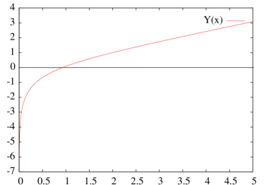
Figure 1: (Color online) Plot of the auxiliary function $Y(x)$ defined in Eq. (23a) as obtained by numerical integration.

The limit $J^{\prime}/J\to 0$ always probes the RC regime (6) provided the underlying two-dimensional subsystem is not quantum disordered, i.e., it satisfies the condition $g<g^{\ }_{c}$. The limit $J^{\prime}/J\to 0$ can only probe the QC regime (7) or the QD regime (8) after fine tuning. This is so because, for any value $g/g^{\ }_{c}\neq 1$, the unconstrained limit $J^{\prime}/J\to 0$ brings the quasi-two-dimensional system either in the regime (6), that is dominated by two-dimensional classical fluctuations, when $g/g^{\ }_{c}<1$ or in the quasi-two-dimensional paramagnetic phase, that is dominated by two-dimensional quantum fluctuations at very low temperatures, when $g/g^{\ }_{c}>1$. When $g/g^{\ }_{c}<1$, the QC regime (7) can only be probed in the $J^{\prime}/J\to 0$ limit if the ratio of length scales

$$R^{\ }_{-}:=\frac{cN/(4\pi\widetilde{\rho}^{\ }_{s})}{\xi^{\prime}}$$ (24a)

is held fixed. When $$g/g^{\ }_{c}>1 J^{\prime}/J\to 0$$, the QC regime (7) or the QD regime (8) can only be probed in the limit if the ratio of length scales

$$R^{\ }_{+}:=\frac{c/\Delta}{\xi^{\prime}}$$ (24b)

is held fixed. In the latter case, the magnitude of $R^{\ }_{+}$ distinguishes the fate of the limit $J^{\prime}/J\to 0$, i.e., whether the onset of AF long-range order is characterized by the quantum fluctuations of regime (7) or the quantum fluctuations of regime (8). When $R^{\ }_{+}$ is below the threshold value of $\pi/4$, we shall see that three-dimensional AF long-range order is impossible down to and at zero temperature (see Fig. 2).

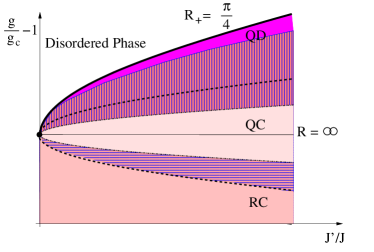
Figure 2: (Color online) Projection of the phase diagram of the quasi-two-dimensional QNLSM into the plane spanned by $g/g_{c}-1$ and $J^{\prime}/J$. The upper bold line is the phase boundary between the AF ordered and the paramagnetic phases corresponding to the fixed ratio $R_{+}=\pi/4$. The hatched regions denote the crossover between the QD and QC regimes, on the one hand, and between the QC and RC regimes, on the other hand. Each curve represents a possible trajectory with fixed $R_{\pm}$ used in order to construct the scaling functions in the limit $J^{\prime}/J\to 0$; the temperature along the curves is always fixed to $T_{AF}$.

IV.1 RC regime

When $g<g^{\ }_{c}$ and $c\beta^{\ }_{AF}\ll\xi^{\prime}$, Eq. (21) simplifies to

$$\frac{c\beta^{\ }_{AF}}{\xi^{\prime}}\simeq\exp\left(-\frac{2\pi\widetilde{\rho}^{\ }_{s}\beta^{\ }_{AF}}{N}\right).$$ (25)

Observe that, for any finite $\widetilde{\rho}^{\ }_{s}$, the condition (6) is always met for $J^{\prime}$ small enough, as, in the limit $J^{\prime}/J\rightarrow 0$, Eq. (25) has the solution

$$\beta^{\ }_{AF}(J^{\prime}/J)\simeq\frac{N}{2\pi\widetilde{\rho}^{\ }_{s}}\left[\frac{1}{2}\ln\left(\frac{J}{J^{\prime}}\right)+\ln\left(\frac{4\pi\widetilde{\rho}^{\ }_{s}/N}{c\ln(J/J^{\prime})}\right)\right]$$ (26)

with corrections of order $\frac{\ln\ln(J/J^{\prime})}{\ln(J/J^{\prime})}$. The dependence of the Néel temperature on $J^{\prime}/J$ shows an essential singularity at $J^{\prime}/J=0$; expansion (26) is very poor.

IV.2 QC regime

When $g<g^{\ }_{c}$ and $c\beta^{\ }_{AF}/\xi^{\prime}\lesssim x^{\ }_{0}$, Eq. (21) becomes

$$\frac{c\beta^{\ }_{AF}}{\xi^{\prime}}\simeq\frac{x^{\ }_{0}}{1+1/(2y^{\ }_{1}R^{\ }_{-})},\qquad R^{\ }_{-}=\frac{cN}{4\pi\widetilde{\rho}^{\ }_{c}\xi^{\prime}}.$$ (27)

Equation (27) is self-consistent with the assumption $c\beta^{\ }_{AF}/\xi^{\prime}\lesssim x^{\ }_{0}$ provided $R^{\ }_{-}\gg 1$. The Néel temperature can be expanded in a power series in $1/R^{\ }_{-}$ when approaching the two-dimensional quantum critical point $\widetilde{\rho}^{\ }_{s}=0$ from the two-dimensional quantum ordered side.

If $g>g^{\ }_{c}$ and $c\beta^{\ }_{AF}/\xi^{\prime}\gtrsim x^{\ }_{0}$, Eq. (22) can be rewritten as

$$\frac{c\beta^{\ }_{AF}}{\xi^{\prime}}\simeq\frac{x^{\ }_{0}}{1-1/(2y^{\ }_{1}R^{\ }_{+})},\qquad R^{\ }_{+}=\frac{c}{\Delta\xi^{\prime}}.$$ (28)

In order for Eq. (28) to be consistent with the assumption $c\beta^{\ }_{AF}/\xi^{\prime}\gtrsim x^{\ }_{0}$, we have to require $R^{\ }_{+}\gg 1$. Again, the Néel temperature can be expanded in a power series in $1/R^{\ }_{+}$ when approaching the two-dimensional quantum critical point $\Delta=0$ from the two-dimensional quantum disordered side.

IV.3 QD regime

When $g>g^{\ }_{c}$ and $c\beta^{\ }_{AF}\gg\xi^{\prime}$, Eq. (22) simplifies to

$$\frac{c\beta^{\ }_{AF}}{\xi^{\prime}}\simeq\sqrt{\frac{2\gamma}{\frac{4}{\pi}-\frac{1}{R^{\ }_{+}}}},\qquad R^{\ }_{+}=\frac{c}{\Delta\xi^{\prime}},$$ (29)

provided $R^{\ }_{+}>\pi/4$. When $R^{\ }_{+}\leq\pi/4$, the Néel temperature is predicted to vanish in the $N=\infty$ approximation. The minimal interlayer coupling $J^{\prime}_{c}$ for which the three-dimensional Néel state exists can be obtained by solving Eq. (29) at $\beta^{\ }_{AF}=\infty$. This gives

$$\frac{J^{\prime}_{c}}{J}=\left(\frac{\pi}{4}\frac{\Delta}{c}\right)^{2}.$$ (30)

IV.4 Critical coupling

The critical coupling $g^{\ }_{c}$ defined in Eq. (21b) separates the Néel ordered phase from the paramagnetic phase of the two-dimensional system at zero temperature. We have seen that the quasi-two-dimensional ordered phase can exist in the limit $J^{\prime}/J\to 0$ even though $g>g^{\ }_{c}$, provided the two-dimensional quantum gap $\Delta$ is scaled accordingly. This implies that any finite coupling $J^{\prime}/J$ between planes renormalizes $g_{c}$ to a larger value $\widetilde{g}^{\ }_{c}$. The $N=\infty$ approximation for $\widetilde{g}^{\ }_{c}$ can be obtained from Eq. (29) after inserting in $c/\xi^{\prime}=\pi\Delta/4$ the renormalized gap $\Delta$ from Eq. (22b). One finds the dependence on $J^{\prime}/J$,

$$\frac{1}{\widetilde{g}^{\ }_{c}}\simeq\frac{1}{g^{\ }_{c}}-\frac{1}{\pi^{2}}\sqrt{\frac{J^{\prime}}{J}}+\cdots,$$ (31)

that is characterized by an essential singularity at $J^{\prime}/J=0$. The boundaries (26) and (31) are depicted in Fig. 3.

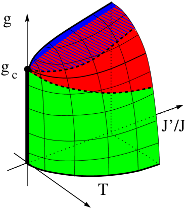
Figure 3: (Color online) Boundaries between the AF ordered and the paramagnetic phase as a function of the spatial anisotropy. The dependence on $J^{\prime}/J$ of the two boundaries (thick lines), one emanating from the origin $(g,T)=(0,0)$ into the plane $g=0$, the other emanating from the two-dimensional quantum critical point $(g,T)=(g^{\ }_{c},0)$ into the plane $T=0$, are given by Eqs. (26) and (31), respectively. The curves on the critical surface (dashed lines) lead to the QC (lower line) and QD (upper line) behaviors.

V Scaling laws in the $N=\infty$ limit

We are now going to verify the claims (9), (11), and (12) in the $N=\infty$ approximation.

V.1 First scaling law

One way to proceed in the case of Eq. (9) is as follows. We solve the saddle-point equation (18) a first time with $\lambda^{\ }_{*}=0$ but $J^{\prime}/J>0$ to determine the Néel temperature, as was done in Sec. IV. We then solve the saddle-point equation (18) a second time but now with $\lambda^{\ }_{*}=J^{\prime}/J=0$ to extract the two-dimensional correlation length $\xi^{(2)}(\beta^{\ }_{AF})$ at the Néel temperature, which in turn determines $\chi^{(2)}_{s}(\beta^{\ }_{AF})$. Alternatively, we can extract $\xi^{(2)}(\beta^{\ }_{AF})$ from

$$\widehat{G}^{(0)}_{j,j}\Big{(}x,x;\lambda=0\Big{)}=\left.\widehat{G}^{(0)}_{j,j}\left(x,x;\left(\xi^{(2)}\right)^{-2}\right)\right|^{\ }_{\alpha=0},$$ (32)

where a matrix element of the $N=\infty$ approximation to the propagator $\widehat{G}^{(0)}$ is explicitly given in Eq. (18c). This equation has the advantage of being cutoff independent in the Pauli-Villars regularization scheme.

After summing over the frequencies and integrating over the two-dimensional momenta, Eq. (32) reduces to

$$\frac{\xi^{\prime}}{\xi^{(2)}(\beta^{\ }_{AF})}=2\left(\frac{\xi^{\prime}}{c\beta^{\ }_{AF}}\right)\operatorname{arcsinh}\left(\frac{1}{2}e^{Y\big{(}c\beta^{\ }_{AF}/\xi^{\prime}\big{)}}\right).$$ (33)

We insert this ratio into

$$J^{\prime}\chi^{(2)}_{s}(\beta^{\ }_{AF})=J^{\prime}\times\frac{S^{2}g}{Nc}\left(\xi^{(2)}(\beta^{\ }_{AF})\right)^{2}$$ (34)

where we made use of Eq. (17) using the $N=\infty$ approximation of the Green function with $\alpha=0$. After trading $J^{\prime}$ for $J$ and $\xi^{\prime}$ defined in Eq. (5a), we find

$$J^{\prime}\chi^{(2)}_{s}(\beta^{\ }_{AF}) = \frac{S^{2}gJ}{Nc}\left(\frac{\xi^{(2)}(\beta^{\ }_{AF})}{\xi^{\prime}}\right)^{2}$$ (35)

$$= \frac{\big{(}c\beta^{\ }_{AF}/\xi^{\prime}\big{)}^{2}}{4\operatorname{arcsinh}^{2}\left(e^{Y\big{(}c\beta^{\ }_{AF}/\xi^{\prime}\big{)}}/2\right)}.$$ (36)

Equation (36) tells us that the function $J^{\prime}\chi^{(2)}_{s}$ is a scaling function of the scaling variable $c\beta^{\ }_{AF}/\xi^{\prime}$. This is not $F^{\ }_{1}$ from Eq. (9), since we are looking for a function of $c\beta^{\ }_{AF}/\xi^{(2)}(\beta^{\ }_{AF})$ and its limiting value when $J^{\prime}/J\to 0$ has yet to be taken.

V.1.1 Renormalized classical regime

In the RC regime (6), where $c\beta^{\ }_{AF}/\xi^{\prime}\ll 1$, and after expanding the right-hand side of Eq. (33) in powers of $c\beta^{\ }_{AF}/\xi^{\prime}$, we get

$$\frac{\xi^{\prime}}{\xi^{(2)}(\beta^{\ }_{AF})}\simeq 1+\frac{1}{24}\left(\frac{c\beta^{\ }_{AF}}{\xi^{\prime}}\right)^{2}+\cdots$$ (37)

and from Eq. (36)

$$J^{\prime}\chi^{(2)}_{s}(\beta^{\ }_{AF})=1-\frac{1}{12}\left(\frac{c\beta^{\ }_{AF}}{\xi^{\prime}}\right)^{2}+\cdots.$$ (38)

According to Eq. (37), we can replace $\xi^{\prime}$ by $\xi^{(2)}(\beta^{\ }_{AF})$ in Eq. (38) to the first nontrivial order,

$$J^{\prime}\chi^{(2)}_{s}(\beta^{\ }_{AF})=1-\frac{1}{12}\left(\frac{c\beta^{\ }_{AF}}{\xi^{(2)}(\beta^{\ }_{AF})}\right)^{2}+\cdots.$$ (39)

We conclude that, in the $N=\infty$ limit, $J^{\prime}\chi^{(2)}_{s}(\beta^{\ }_{AF})$ equals the scaling function

$$\mathcal{F}^{(\mathrm{RC})}_{1}(x):=1-\frac{x^{2}}{12}+\cdots$$ (40a)

with the scaling variable

$$x:=\frac{c\beta^{\ }_{AF}}{\xi^{(2)}(\beta^{\ }_{AF})}$$ (40b)

in the RC regime (6). The universal scaling function $F_{1}$ is then obtained from $\mathcal{F}^{\mathrm{RC}}_{1}(x)$ taking the limit $J^{\prime}/J\to 0$. Observe that we do not expect the function $\mathcal{F}^{\mathrm{RC}}_{1}(x)$ to be universal in general. For example, this function is modified by adding longer range interlayer couplings in Eq. (13d).footnote: nnn nnnn etc

For comparison with numerical simulations, it is instructive to compute this relation as a function of $\alpha=J^{\prime}/J$. Inserting the Néel temperature from Eq. (26) in Eq. (39) leads to

$$J^{\prime}\chi^{(2)}_{s}(\beta^{\ }_{AF})\simeq 1-\frac{1}{12}\frac{c^{2}N^{2}}{\left(4\pi\widetilde{\rho}^{\ }_{s}\right)^{2}}\frac{J^{\prime}}{J}\ln^{2}\left(\frac{J}{J^{\prime}}\right)+\cdots.$$ (41)

The universal value in the limit $J^{\prime}/J\rightarrow 0$ is thus established, since

$$F^{\ }_{1}(0)=1$$ (42a)

is independent of any microscopic details, i.e., the spin stiffness $$\widetilde{\rho}^{\ }_{s} c$$ or the spin-wave velocity . For comparison, the RPA predicts

$$F^{\mathrm{(RPA)}}_{1}(0)=1/2,$$ (42b)

while the MC calculations from Ref. Yasuda05, gives

$$F^{\mathrm{(MC)}}_{1}(0)\simeq 0.77.$$ (42c)

We show in Appendix A that the form of the nonuniversal corrections in Eq. (41) are similar to the corrections obtained in the quasi-one-dimensional Ising model.

The factor $cN/(4\pi\widetilde{\rho}^{\ }_{s})$ scales as $1/S$. As expected, the nonuniversal corrections get smaller for bigger spins. We show in Sec. VI that the nonuniversal corrections vanish in the $N=\infty$ approximation to the classical Heisenberg AF.

The result (41) is only reliable for very small $J^{\prime}/J$, due to the limited quality of the approximation (26). To compare the $N=\infty$ approximation with MC simulations, it is best to rely on a numerical solution of Eq. (25) for the Néel temperature. As can be seen from Fig. 4, for $J^{\prime}/J<0.1$, the $N=\infty$ approximation (39) of the first scaling law obeys a limiting behavior as $J^{\prime}/J\rightarrow 0$ similar to the MC results from Ref. Yasuda05, . For $J^{\prime}/J>0.1$, the magnitude of the deviation of the effective coordination number from its universal asymptotic value as $J^{\prime}/J\to 0$ can be explained using the empirical formula for the Néel temperature proposed in Ref. Yasuda05, . However, the sign of the nonuniversal correction in Eq. (39) is wrong. We do not expect the quasi-two-dimensional QNLSM used here to be valid for the description of the system at $J^{\prime}/J>0.1$ as the effective interlayer separation $\xi^{\prime}$ is only a few lattice spacing large. Instead, it is likely that it is necessary to also consider the lattice structure of the system in each plane to obtain an appropriate description.

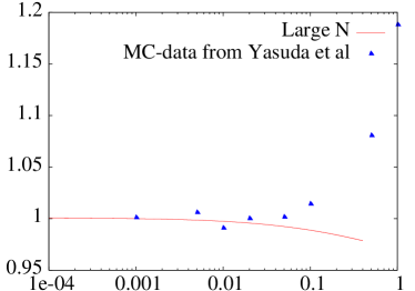
Figure 4: (Color online) The scaling function $F^{\ }_{1}$ is plotted vs $J^{\prime}/J$ for spin $1/2$. The curve represents the $N=\infty$ approximation (39), with the Néel temperature obtained from numerical solution of Eq. (25). The points are the MC data from Yasuda et al. in Ref. Yasuda05, . In both cases, the normalization is such that the curves go through 1 for $J^{\prime}/J=10^{-3}$.

V.1.2 Quantum critical regime

The condition $\Delta=0$ fine tunes the underlying two-dimensional system to be at a quantum critical point. From Eqs. (22) and (23b), we then have $c\beta^{\ }_{AF}/\xi^{\prime}=x^{\ }_{0}$. Taking advantage of this relation in Eq. (33) gives

$$\frac{\xi^{\prime}}{\xi^{(2)}(\beta^{\ }_{AF})}=\frac{\Theta}{x^{\ }_{0}},$$ (43a)

where

$$\Theta:=2\ln\frac{1+\sqrt{5}}{2}.$$ (43b)

The right-hand side of Eq. (35) thus becomes

$$J^{\prime}\chi^{(2)}_{s}(\beta^{\ }_{AF}) = \frac{x^{2}_{0}}{\Theta^{2}}.$$ (44)

Chubukov et al. in Ref. Chubukov94, have shown that

$$\frac{c\beta}{\xi^{(2)}(\beta)}=\Theta$$ (45)

in the $N=\infty$ approximation when $\Delta=0$. The universal function $F^{\ }_{1}$ from Eq. (9) thus takes the value

$$F^{\ }_{1}(\Theta)=\frac{x^{2}_{0}}{\Theta^{2}}.$$ (46)

exactly at the QC point $\Delta=0$.

In the scaling limit $J^{\prime}/J\to 0$ with the ratios $R^{\ }_{\mp}$ from Eqs. (24a) and (24b) held fixed, Eqs. (43a) and (44) become

$$\frac{\xi^{\prime}}{\xi^{(2)}(\beta^{\ }_{AF})}=\frac{\Theta}{x^{\ }_{0}}+\frac{\kappa}{R^{\ }_{\mp}}+\mathcal{O}\big{(}R^{-2}_{\mp}\big{)}$$ (47)

and

$$J^{\prime}\chi^{(2)}_{s}(\beta^{\ }_{AF})=\frac{x^{2}_{0}}{\Theta^{2}}-\frac{\kappa}{R^{\ }_{\mp}}+\mathcal{O}\big{(}R^{-2}_{\mp}\big{)},$$ (48)

respectively, where

$$\kappa:=\frac{\Theta+2y^{\ }_{1}/\sqrt{5}}{x^{\ }_{0}}.$$ (49)

V.1.3 Quantum disordered regime

We close with the QD regime (8) for which $c\beta^{\ }_{AF}/\xi^{\prime}\gg 1$. The underlying two-dimensional system is in its quantum disordered phase with

$$\xi^{(2)}(T=0)=c/\Delta.$$ (50)

Taking the scaling limit $J^{\prime}/J\to 0$ with the ratio $R^{\ }_{+}$ from Eq. (24b),

$$R^{\ }_{+} = \frac{c}{\Delta\xi^{\prime}}$$ (51)

$$= \xi^{(2)}(T=0)/\xi^{\prime}$$

$$= \xi^{(2)}(\beta^{\ }_{AF})/\xi^{\prime}+\mathcal{O}\left(e^{-c\beta^{\ }_{AF}/\Delta}\right),$$

held fixed turns Eq. (35) into

$$J^{\prime}\chi^{(2)}(\beta^{\ }_{AF})\simeq R^{2}_{+}$$ (52)

up to exponentially small corrections in $(R^{\ }_{+}-\pi/4)^{-1/2}$.

V.1.4 Summary

To sum up, we have the $N=\infty$ approximation

$$\lim_{J^{\prime}/J\to 0}J^{\prime}\chi^{(2)}(\beta^{\ }_{AF})\simeq\left\{\begin{array}[]{ll}1,&\mbox{ RC regime},\\ &\\ \frac{x^{2}_{0}}{\Theta^{2}}-\frac{\kappa}{R^{\ }_{\mp}},&\mbox{ QC regime},\\ &\\ R^{2}_{+},&\mbox{ QD regime},\end{array}\right.$$ (53)

to the first universal function (9), where $R^{\ }_{\mp}\gg 1$ in the QC regime while $R^{\ }_{+}\gtrsim\pi/4$ in the QD regime. The result $F^{\ }_{1}(0)=1$ is exact in the RG regime (9). The result $F^{\ }_{1}\big{(}c\beta^{\ }_{AF}/x^{(2)}(\beta^{\ }_{AF})\big{)}=\frac{x^{2}_{0}}{\Theta^{2}}-\frac{\kappa}{R^{\ }_{\mp}}$ is accurate up to corrections of order $R^{-2}_{\mp}$ in the QC regime (6). The result $F^{\ }_{1}\big{(}c\beta^{\ }_{AF}/x^{(2)}(\beta^{\ }_{AF})\big{)}=R^{2}_{+}$ is accurate up to exponentially small corrections in $(R^{\ }_{+}-\pi/4)^{-1/2}$ in the QD regime (7). The RC regime (8) is the only one for which we were able to compute the nonuniversal corrections to the limit $J^{\prime}/J\to 0$. They are of second order in the variable $c\beta^{\ }_{AF}/\xi^{(2)}(\beta^{\ }_{AF})$ but nonanalytic in the variable $J^{\prime}/J$, namely of order $(J^{\prime}/J)\ln^{2}(J/J^{\prime})$.

V.2 Second scaling law

The second universal scaling law (11), which involves the three-dimensional spin susceptibility, is established as follows. In the $N=\infty$ approximation,

$$\chi^{(3)}\big{(}\pi,\pi,0,\omega=0;\beta^{\ }_{AF}\big{)}=\frac{S^{2}g}{cN}\frac{1}{4\alpha},$$ (54)

which immediately leads to the second universal relation

$$J^{\prime}\chi^{(3)}_{s}(\beta^{\ }_{AF})=\frac{1}{4},$$ (55)

in the RC, QC, and QD regimes.

V.3 Third scaling law

We close by establishing the third universal scaling law (12), which involves the instantaneous structure factor. We insert the definition (17) in Eq. (12b), and use the $N=\infty$ approximation to the correlation function. After performing the frequency integration, we find

$$S(\boldsymbol{k}^{\ }_{AF},k^{\ }_{z}=0,t=0;\beta)=\frac{S^{2}g}{4N}\xi^{\prime}\coth\big{(}c\beta/\xi^{\prime}\big{)}.$$ (56)

The last universal relation is then established,

$$\beta^{\ }_{AF}J^{\prime}S(\boldsymbol{k}^{\ }_{AF},k^{\ }_{z}=0,t=0;\beta^{\ }_{AF})=\mathcal{F}^{\ }_{3}\big{(}c\beta^{\ }_{AF}/\xi^{\prime}\big{)},$$ (57a)

where in the $$N=\infty$$ approximation,

$$\mathcal{F}^{\infty}_{3}(x):=\frac{x}{4}\coth x$$ (57b)

and

$$x:=\frac{c\beta^{\ }_{AF}}{\xi^{\prime}}.$$ (57c)

The universal scaling function $F_{3}$ is then obtained from $\mathcal{F}^{\infty}_{3}(x)$ taking the limit $J^{\prime}/J\to 0$. As for the first scaling law, we do not expect the function $\mathcal{F}^{\infty}_{3}(x)$ to be universal in general. The behavior of $\mathcal{F}^{\infty}_{3}(x)$ when $x\ll 1$, $x\sim 1$, and $x\gg 1$ distinguishes the RC, QC, and QD regimes. Observe in this context that, as $\mathcal{F}^{\infty}_{3}(x)\rightarrow 1/4+\mathcal{O}(x^{2})$ in the limit of small $x$, the function $F^{\ }_{3}$ is the same as $F^{\ }_{2}$ in the RC regime, as expected from the quasielastic approximation Birgeneau71 ; Keimer92

$$\chi(\boldsymbol{q},\omega=0;\beta)\simeq-\beta S(\boldsymbol{q},t=0;\beta).$$ (58)

In the QD regime, the scaling variable $x$ can become arbitrary large as $R_{+}\to\pi/4$. [In particular, this is the case when $J^{\prime}\to J^{\prime}_{c}$, see Eq. (30).] Consequently, the function $\mathcal{F}^{\ }_{3}(x)\simeq x/4$ on the right hand side of Eq. (57a) diverges when the ratio $R^{\ }_{+}$ that defines how the limit $J^{\prime}\to 0$ is taken approaches $\pi/4$.

VI Scaling laws in the $N=S=\infty$ limit

The three components of the spin operators with spin quantum number $S$ commute in the limit $S\to\infty$. The results of Yasuda et al. suggest that the effective coordination number (2) is independent of $S$ in the limit $J^{\prime}/J\to 0$. This limiting value of the effective coordination number is thus the same irrespective of $S$ taking values deep in the quantum regime, $S=1/2$, or classical regime, $S=\infty$. If so, it is instructive to compare our analysis of the quasi-two-dimensional QNLSM (13b) with that of the quasi-two-dimensional NLSM. The action of the quasi-two-dimensional NLSM is obtained from Eq. (13b) by dropping all references to the imaginary time, setting $S=1$ and $c=1$, and replacing the integral over $\tau$ by $1/T$,

$$S[\boldsymbol{\sigma}]:=\frac{\rho^{\ }_{s}}{2T}\sum_{j}\int d^{2}\boldsymbol{x}\,\left[\big{(}\nabla\boldsymbol{\sigma}_{j}\big{)}^{2}+\frac{J^{\prime}}{J}\boldsymbol{\sigma}_{j}\cdot\boldsymbol{\sigma}_{j+1}\right]$$ (59)

with $\rho^{\ }_{s}\equiv J$. Again, the constraint $\boldsymbol{\sigma}^{2}_{j}(\boldsymbol{x})=1$ can be removed in favor of the Lagrange multiplier $\lambda$. If the original fields $\boldsymbol{\sigma}$ are integrated out, one obtains the effective action

$$S^{\ }_{\mathrm{eff}}[\lambda]=-\frac{1}{2gT}\sum_{j}\int d^{2}x\,\lambda^{\ }_{j}+\frac{1}{2}\operatorname{Tr}\ln\big{(}-\boldsymbol{\nabla}^{2}-\alpha\Delta^{\ }_{z}+\lambda^{\ }_{j}\big{)}$$ (60a)

where

$$g=N/\rho^{\ }_{s}$$ (60b)

that should be compared with Eqs. (14b) and (14c). The spin susceptibility is now related to the two-point correlation functions by

$$\chi^{(3)}(\boldsymbol{k}+\boldsymbol{k}_{AF},\pi+k_{z};\beta)=\frac{g}{N}G(\boldsymbol{k},k_{z};\beta)$$ (61)

that should be compared with Eq. (17).

To compute the first scaling law in the $N=\infty$ approximation, we proceed as in the quantum case. We thus solve directly the classical counterpart to Eq. (32) for the ratio $\xi^{\prime}/\xi^{(2)}$ with $\xi^{(2)}$ evaluated at the Néel temperature. We find

$$\frac{\xi^{\prime}}{\xi^{(2)}(\beta^{\ }_{AF})}=1.$$ (62)

Hence the first scaling law in the $N=\infty$ approximation simply reads

$$J^{\prime}\chi^{(2)}_{s}(\beta^{\ }_{AF})=\mathcal{F}^{\ }_{1}(x)$$ (63a)

with

$$\mathcal{F}^{\ }_{1}(x)=1$$ (63b)

and

$$x=\frac{J\beta^{\ }_{AF}a}{\xi^{(2)}(\beta^{\ }_{AF})}.$$ (63c)

The counterpart to the universal function (9) obtained in the limit $J^{\prime}/J\rightarrow 0$ is then

$$F^{\ }_{1}(x)=1.$$ (64)

It agrees with the RC limit (42a). This is consistent with the MC study from Yasuda et al. in Ref. Yasuda05, . Contrary to the quantum case, nonuniversal corrections are absent in the saddle-point approximation. This result is also consistent with the observation from Ref. Yasuda05, that the finite $J^{\prime}/J$ nonuniversal corrections decrease with increasing $S$.

We turn to the second scaling law. Inserting the $N=\infty$ approximation of the two-point correlation function in Eq. (61) at the wave vector $(\pi,\pi,0)$ leads to

$$J^{\prime}\chi_{s}^{(3)}(\beta^{\ }_{AF})=\frac{1}{4},$$ (65)

as in the quantum case.

There is no independent third scaling law in classical thermodynamic equilibrium since all observables are time independent by assumption.

VII Comparison of the scaling laws with experiments

Many quasi-two-dimensional quantum Heisenberg AF are now available. Neutron studies have been performed on compounds with spin $S=1/2$ [La₂CuO₄ in Refs. Birgeneau99, and Toader05, , Sr₂CuO₂Cl₂ in Refs. Borsa92, and Greven95, , and copper formate tetradeuterate (CFTD) in Ref. Ronnow99, ] spin $S=1$ (La₂NiO₄ in Ref. Nakajima95, and K₂NiF₄ in Ref. Greven95, ), as well as spin $S=5/2$ (KFeF₄ in Ref. Fulton94, and Rb₂MnF₄ in Refs. Lee98, and Leheny99, ). All these materials are good realizations of the two-dimensional QNLSM above their ordering temperature $T^{\ }_{AF}$. In particular, the temperature dependence of the correlation length in these systems is well explained (without free parameter) by the correlation length of the two-dimensional QNLSM in the RC regime and at the three-loop order, Chakravarty88 ; Chakravarty89 ; Chubukov94 ; Hasenfratz91

$$\frac{\xi^{(2)}(T)}{a}=\frac{e}{8}\frac{c/a}{2\pi\rho_{s}}e^{2\pi\rho_{s}/T}\left[1-\frac{1}{2}\left(\frac{T}{2\pi\rho_{s}}\right)+\cdots\right].$$ (66)

All these systems have an interplane exchange coupling $J^{\prime}/J$ which is much smaller than the spin anisotropy. The latter is either of $XY$ type (for the $S=1/2$ systems listed above) or Ising type (for the remaining examples chosen). Hence the onset of AF magnetic long-range order at $T^{\ }_{AF}$ is a classical critical point that belongs to the $XY$ or Ising universality class. Moreover, $T^{\ }_{AF}$ is mainly determined by the (lower) critical temperature of the two-dimensional system, which is finite in opposition to that for the spin-isotropic two-dimensional quantum Heisenberg AF. For this reason, we do not believe that the scaling laws derived above for a spin-isotropic quantum Heisenberg AF can be observed in the materials mentioned above.

A family of organic quasi-two-dimensional quantum AF has been synthesized with the general chemical formula A₂CuX₄, where A=5CAP (5CAP stands for 2-amino-5-chloropyridinium) or A=5MAP (5MAP stands for 2-amino-5-methylpyridinium), and X=Br or Cl. Woodward02 The AF Heisenberg exchange coupling $J$ in these materials is between 6 and $10K$, and they have a Néel temperature of about $T_{AF}\simeq 0.6J$. According to Ref. Woodward02, , the dominant subleading term in the Hamiltonian describing their magnetic response is the interlayer Heisenberg exchange coupling $J^{\prime}$. The rationale for $J^{\prime}$ being the leading subdominant term to the planar $J$ is the following mean-field argument. Woodward02 Consider the compound La₂CuO₄ as an example of a layered structure in which adjacent layers are staggered, i.e., there exists a relative in-plane displacement $(1/2,1/2)$ between any two neighboring layers. Each in-plane ion has thus four equidistant neighbors in the layer directly above it. Assume that, in any given layer, the spin degrees of freedom occupy the sites of a square lattice and that they are frozen in a classical Néel configuration. Any in-plane spin has then four nearest-neighbors in the layer above it whose net mean field vanishes. In contrast, the stacking of planes is not staggered in the organic quasi-two-dimensional AF described in Ref. Woodward02, , so that this cancellation mechanism does not work. Consequently, the ratio $J^{\prime}/J$ is expected to be much larger for A₂CuX₄ than for La₂CuO₄.

The interlayer exchange parameter for A₂CuX₄ is estimated in Ref. Woodward02, to be $J^{\prime}/J\simeq 0.08$ with the help of the formula

$$T^{\ }_{AF}=zJ^{\prime}S(S+1)\big{[}\xi^{(2)}(T^{\ }_{AF})/a\big{]}^{2}.$$ (67)

Equation (67) can be found in Ref. Chakravarty88, while its quasi-one-dimensional version was obtained by Villain and Loveluck in Ref. Villain77, . The Néel temperature of the spin-1/2 quasi-two-dimensional Heisenberg model is hereby estimated by balancing the thermal energy $T^{\ }_{AF}$ against the gain in Zeeman energy obtained by aligning a planar spin $S(S+1)$ along a mean-field magnetic field of magnitude $zJ^{\prime}[\xi^{(2)}(T^{\ }_{AF})/a]^{2}$ that points parallel to the stacking direction. Here $\xi^{(2)}(T_{AF})$ is the two-dimensional correlation length estimated at the Néel temperature from formula (66) and $z$ is the coordination number of layers. Using their empirical formula (which is consistent with the first scaling law in the limit $J^{\prime}/J\to 0$), Yasuda et al. in Ref. Yasuda05, claim the three times larger value $J^{\prime}/J\simeq 0.24$. This discrepancy is explained in Appendix B. To our knowledge, there is no independent estimate for the interlayer coupling $J^{\prime}/J$ deduced from measuring the spin-wave velocity for A₂CuX₄. We are also not aware of measurements of the correlation length above the critical temperature for A₂CuX₄.

VII.1 Experimental discussion of the first scaling law

The two-dimensional spin susceptibility is inaccessible to a direct measurement at the Néel temperature, the temperature at which our scaling laws hold. This is not to say that the two-dimensional spin susceptibility is inaccessible at all temperatures. In fact, one would expect a window of temperature above the Néel temperature for which the three-dimensional spin susceptibility is well approximated by the two-dimensional one in a good quasi-two-dimensional AF magnet. If so one could try to test the first scaling law by extrapolation from high temperatures.

To this end, we could first attempt to use the measured values of the Néel temperature and of the anisotropic spin-wave dispersion together with computations of the two-dimensional spin-wave velocity $c$ and spin stiffness $\rho^{\ }_{s}$ from first principle, to test the accuracy of the prediction (37) for the ratio

$$\Xi:=\frac{\xi^{(2)}(T^{\ }_{AF})}{\xi^{\prime}}$$ (68)

between the two-dimensional correlation length $\xi^{(2)}(T^{\ }_{AF})$ and the effective interlayer spacing (5a). Indeed, it is reassuring to know that there exists a good agreement between formula (66) and measurements of the correlation length above $T^{\ }_{AF}$ in the RC regime.

Needed are the numerator and denominator in the RC regime of the right-hand side of Eq. (68) expressed as a function of $N$, $c$, $\rho^{\ }_{s}$, and $T^{\ }_{AF}$ to first order in the $1/N$ expansion. The two-dimensional correlation length is Chubukov94

$$\frac{\xi^{(2)}(T)}{a}=\xi^{\ }_{0}\frac{c/a}{T}\left(\frac{(N-2)T}{2\pi\rho^{\ }_{s}}\right)^{1/(N-2)}\exp{\frac{2\pi\rho^{\ }_{s}}{(N-2)T}},$$ (69a)

where the constant

$$\xi^{\ }_{0}=\big{(}e/8\big{)}^{1/(N-2)}\Gamma\big{(}1+1/(N-2)\big{)}$$ (69b)

depends on $e=2.718...$ and the Gamma function. The Néel temperature is the implicit solution to Irkhin97

$$\frac{4\pi\rho^{\ }_{s}}{(N-2)T^{\ }_{AF}} = \ln\frac{T^{2}_{AF}}{c^{2}/a^{2}}+\frac{2}{N-2}\ln\frac{4\pi\rho_{s}}{(N-2)T^{\ }_{AF}}$$ (70a)

$$+\frac{1.012}{N-2}+\ln\frac{1}{\mathcal{Z}^{\prime}}+\ln\frac{J}{J^{\prime}}$$

with

$$\mathcal{Z}^{\prime} = \left(1-\frac{8}{3\pi^{2}N}\ln\frac{c\Lambda N}{16\rho^{\ }_{s}}\right)$$ (70b)

$$\times\left(1+\frac{1.069}{N}\right)\left(\frac{(N-2)T}{4\pi\rho^{\ }_{s}}\right)^{1/(N-2)}.$$

The dependence on the momentum cutoff $\Lambda$ of the two-dimensional correlation length occurs through $\xi^{\prime}$ only,

$$\frac{\xi^{(2)}(T^{\ }_{AF})}{a}=\xi^{\ }_{0}\left(2e^{0.506}\right)^{1/(N-2)}\frac{\xi^{\prime}}{a}.$$ (71)

One thus gets the universal number

$$\Xi=\Gamma\big{(}1+1/(N-2)\big{)}\left(\frac{e^{1.506}}{4}\right)^{1/(N-2)}$$ (72)

as it is independent of the spin-wave velocity and the spin stiffness. In particular, $\Xi\approx 1.127$ for $N=3$. (In the $N=\infty$, we found $\Xi=1$.)

We have computed the ratio $\Xi$ for some spin $S=1/2$ quasi-two-dimensional AF using the values of $T^{\ }_{AF}$, $(J^{\prime}/J)^{\ }_{\mathrm{sw}}$, $2\pi\rho^{\ }_{s}$, and $c$ listed in Table 1. Here, $(J^{\prime}/J)^{\ }_{\mathrm{sw}}$ is the ratio of the interplane to the intraplanar exchange couplings deduced from the spin-wave spectra measured using inelastic neutrons scattering at temperatures well below the measured $T^{\ }_{AF}$. The measured value $(J^{\prime}/J)^{\ }_{\mathrm{sw}}$ is interpreted as the multiplicative renormalization

$$\left(\frac{J^{\prime}}{J}\right)^{\ }_{\mathrm{sw}}=\left(1-\frac{8}{3\pi^{2}N}\ln\frac{c\Lambda N}{16\rho^{\ }_{s}}\right)\left(\frac{J^{\prime}}{J}\right)$$ (73)

that arises solely from quantum fluctuations. Irkhin97 In turn, this allows us to express $\xi^{\prime}$ in Eq. (5a) in terms of the microscopic parameters $a$, $\Lambda$, $J$, and $J^{\prime}$ on the one hand, and the macroscopic parameters $\rho^{\ }_{s}$ and $T^{\ }_{AF}$ on the other hand,

$$\frac{\xi^{\prime}}{a} = \left(\frac{J^{\prime}}{J}\right)^{-1/2}_{\mathrm{sw}}\left(1+\frac{1.069}{N}\right)^{-1/2}$$ (74)

$$\times\left(\frac{(N-2)T^{\ }_{AF}}{4\pi\rho^{\ }_{s}}\right)^{-1/[2(N-2)]}.$$

The crossover length scale $\xi^{\prime}$ in Table 1 then follows from inserting $N=3$ and the values for $T^{\ }_{AF}$ and $\rho^{\ }_{s}$ from Table 1. The same is done with Eq. (69a) to obtain $\xi^{(2)}(T^{\ }_{AF})$ in Table 1. One finds the measured values $\Xi^{\ }_{\mathrm{meas}}\approx 0.49$ for La₂CuO₄, $\Xi^{\ }_{\mathrm{meas}}\approx 0.02$ for Sr₂CuO₂Cl₂, and $\Xi^{\ }_{\mathrm{meas}}\approx 0.34$ for CFTD. The smallness of the measured $\Xi^{\ }_{\mathrm{meas}}$ compared to $\Xi\approx 1.127$ indicates that the actual transition to the ordered phase takes place when the two-dimensional correlation length is smaller than the effective interlayer separation $\xi^{\prime}$. This discrepancy with the large-$N$ expansion can be understood as follows. The compounds of Table 1 all have a smaller anisotropy $(J^{\prime}/J)^{\ }_{\mathrm{sw}}$ as compared to the $XY$ anisotropy or to the Dzyaloshinsky-Moria term. Furthermore, the Sr₂CuO₂Cl₂system has about the same critical temperature as the other two compounds, although its anisotropy is three orders of magnitude smaller. This indicates Birgeneau99 ; Toader05 ; Greven95 ; Ronnow99 that the phase transition is not triggered by a pure dimensional crossover but by a combination of a symmetry and dimensional crossover that effectively enhances the true two-dimensional correlation length over that for the pure two-dimensional $O(3)$ QNLSM. The same conclusions may be drawn for systems with higher spins.

We close this section by evaluating the first scaling law in the RC regime to the order $1/N$. The two-dimensional spin susceptibility at the wave vector $(\pi,\pi)$ and at vanishing frequency $\omega=0$ is

$$\chi^{(2)}_{s}(T^{\ }_{AF})=\mathcal{Z}\frac{S^{2}g}{Nc}\left(\frac{\xi^{(2)}(T^{\ }_{AF})}{a}\right)^{2},$$ (75a)

where the two-dimensional multiplicative renormalization $$\mathcal{Z}$$ is Chubukov94 ; footnote: Z

$$\mathcal{Z} = \left(1-\frac{8}{3\pi^{2}N}\ln\frac{c\Lambda N}{16\rho^{\ }_{s}}\right)$$

$$\times\left(1+\frac{0.188}{N}\right)\left(\frac{(N-2)T^{\ }_{AF}}{2\pi\rho^{\ }_{s}}\right)^{1/(N-2)}.$$

Remarkably, the momentum cutoff $\Lambda$ drops from the ratio

$$\frac{\mathcal{Z}}{\mathcal{Z}^{\prime}}=\frac{1+\frac{0.188}{N}}{1+\frac{1.069}{N}}\times 2^{-1/(N-2)}.$$ (76)

For $N=3$, $\mathcal{Z}/\mathcal{Z}^{\prime}=0.391$. (In the $N=\infty$ limit, we find $\mathcal{Z}/\mathcal{Z}^{\prime}=1$.) The $1/N$ correction to the first scaling law thus reads

$$J^{\prime}\chi^{(2)}_{s}(T^{\ }_{AF})=\frac{\mathcal{Z}}{\mathcal{Z}^{\prime}}\Xi^{2}.$$ (77)

For $N=3$, $J^{\prime}\chi^{(2)}_{s}(T^{\ }_{AF})=0.497$. Observe that this is very close to the RPA prediction of $1/2$.

	La2CuO4	Sr2CuO2Cl2	CFTD
	Refs. Birgeneau99, and Toader05,	Ref. Greven95,	Ref. Ronnow99,
$J$	$1566K$	$1450K$	$73.2K$
$T^{\ }_{AF}$	$0.2074J$	$0.1769J$	$0.225J$
$J^{\ }_{XY}/J$	$5.7\times 10^{-4}$	$5.3\times 10^{-4}$
$J_{DM}/J$	$1.5\times 10^{-2}$		$7\times 10^{-2}$
$(J^{\prime}/J)^{\ }_{\mathrm{sw}}$	$5\times 10^{-5}$	$10^{-8}$	$5\times 10^{-5}$
$2\pi\rho_{s}$	$1.131J$	$1.15J$	$1.31J$
$c$	$1.669Ja$	$1.669Ja$	$1.669Ja$
$\xi^{(2)}(T_{AF})$	$105.6a$	$303a$	$69.77a$
$\xi^{\prime}$	$215.81a$	$1.548\times 10^{4}a$	$207.197a$

Table 1: Relevant parameters for some $S=1/2$ quasi-two-dimensional AF. The intraplanar nearest-neighbor AF Heisenberg exchange coupling is $J$, while $J^{\prime}$ is the AF Heisenberg coupling between nearest-neighbor layers. The $XY$ exchange coupling is $J^{\ }_{XY}$, while $J^{\ }_{DM}$ is the coupling of a Dzyaloshinsky-Moriya interaction. The Néel temperature is $T_{AF}$. The two-dimensional spin stiffness $2\pi\rho^{\ }_{s}$ and spin-wave velocity $c$ are obtained either from large $S$ expansions or from MC simulations. The two-dimensional correlation length $\xi^{(2)}(T^{\ }_{AF})$ is obtained from formula (66). Lengths are measured in units of the lattice spacing $a$.

VII.2 Experimental discussion of the third scaling law

What has been extensively studied experimentally is an inelastic neutron-scattering measurement that is believed to yield an approximation to the instantaneous structure factor

$$S^{\ }_{0}(\beta):=\int\limits_{-\infty}^{+\infty}\frac{d\omega^{\prime}}{2\pi}S^{\ }_{0}(\pi,\pi,0,\omega^{\prime};\beta).$$ (78)

Two ranges of temperatures have been studied in the literature. In the 1970s the chosen temperature range was a very narrow one about the AF transition temperature. The rationale for this choice was to study the critical regime surrounding the ordering temperature. In the 1990s the temperature range was broader and above the onset of three-dimensional critical fluctuations.Keimer92 ^-Leheny99 The rationale was primarily to study two-dimensional fluctuations associated with the classical renormalized regime of a two-dimensional AF. In either cases, the experimental measurement of $S^{\ }_{0}(\beta)$ is performed in arbitrary units, i.e., the overall scale of $S^{\ }_{0}(\beta)$ is unknown. Since we are predicting a universal number when measured in some given units, we need to convert any measured number in arbitrary units $S^{(\mathrm{a.u})}_{0}(\beta)$ into a number in some chosen units. We do this by multiplying $S^{(\mathrm{a.u})}_{0}(\beta)$ with a conversion factor,

$$S^{\ }_{0}(\beta)\sim S^{(\mathrm{a.u})}_{0}(\beta)\times\frac{S^{(\mathrm{MC})}_{0}(\beta^{*})}{S^{(\mathrm{a.u})}_{0}(\beta^{*})},$$ (79)

obtained by taking the ratio of the number $S^{(\mathrm{MC})}_{0}(\beta^{*})$ at inverse temperature $\beta^{*}$ computed within some scheme with the measured number in the same arbitrary units $S^{(\mathrm{a.u})}_{0}(\beta^{*})$ at the inverse temperature $\beta^{*}$.

We are only aware of the published MC computation by Kim and Troyer in Ref. Kim98, of the static structure factor at $(\pi,\pi)$ of a spin-1/2 AF on a square lattice. We use this computation at temperatures such that the corresponding correlation length is $3$ in units of the lattice spacing. These are high temperatures for which the two-dimensional static structure factor should be a good approximation to the three-dimensional one. We are not aware of a published calculation of the static structure factor using either MC or high-temperature series expansion for spin-1 or spin-5/2 AF on a square lattice that are needed to reinterpret from our point of view the experiments from Refs. Nakajima95, or Refs. Fulton94, , Lee98, , and Leheny99, , respectively. If we restrict ourselves to the experiments on quasi-two-dimensional spin-$1/2$ from Refs. Birgeneau99, Greven95, , and Ronnow99, , we fail again to observe a signature of universality in $J^{\prime}\beta S^{\ }_{0}(\beta)$ when measured at the temperatures $T=337K,\ 278K,\ 18K$ that are $12K$, $21.5K$, and $1.5K$ above the corresponding ordering temperatures, respectively, as we find that $J^{\prime}\beta S^{\ }_{0}(\beta)$ takes the values $1.17$, $0.001$, and $0.077$, respectively.

VIII Conclusions

As we have seen, interesting scaling relations can be established between the interplane coupling $J^{\prime}$ and observables of the underlying two-dimensional system or the quasi-two-dimensional system. The large-$N$ approximation is particularly well suited to compute the universal functions obtained in the limit $J^{\prime}\rightarrow 0$ at the Néel temperature and derive the leading nonuniversal corrections. The saddle-point approximation already leads to prediction in qualitative agreement with Monte Carlo (MC) simulations. To compare with existing experiments, we have included corrections of order $1/N$. These corrections allow us to take into account the renormalization of the wave function as well as the renormalization of the interlayer coupling, but will probably not affect the qualitative picture obtained in the saddle-point approximation.

The analysis of the quasi-two-dimensional model has revealed the existence of different regimes at low temperatures, corresponding to the renormalized classical (RC), quantum critical (QC), and quantum disordered (QD) regimes of the two-dimensional underlying system. The universal constant obtained from the first and third scaling laws in the limit $J^{\prime}/J\to 0$ are strongly modified depending on the regime considered. For the second scaling law, we did not find any distinction between the three regimes in the saddle-point approximation. However, we expect different corrections for the RC, QC, and QD regimes to the next order in the $1/N$ expansion. While the RC result will probably not be strongly affected by renormalizations, the constant obtained in the quantum regimes might be modified more consequently by higher orders of the $1/N$ expansion.

The first scaling law in the RC qualitatively agrees with the MC simulations of Yasuda et al. in Ref. Yasuda05, for small $J^{\prime}/J<0.1$. Small variations of the Néel temperature are exponentiated in the correlation length. As a consequence, the first scaling law is very sensitive to small errors in the expression for the Néel temperature, so that a quantitative agreement between numerical simulations and our results seems difficult to achieve, even going beyond the saddle-point approximation.

Recent MC simulations of quasi-two-dimensional systems in the RC, QC, and QD regimes have been performed by Yao and Sandvik in order to test the scaling relations described in the present paper. Yao06 Their numerical results share many qualitative properties with our predictions.

It is instructive to view our first scaling law against the mean-field estimate for the Néel temperature Villain77 ; Chakravarty88 obtained by balancing the gain in energy derived from aligning planar spin $S$ with a mean-field magnetic field $SJ^{\prime}[\xi^{(2)}(T)]^{2}$ parallel to the stacking direction with the thermal energy $T$. This would give the naive estimate

$$\frac{J^{\prime}}{J}\left(\frac{\xi^{(2)}(T^{MF}_{AF})}{a}\right)^{2}\sim\frac{T^{MF}_{AF}}{J}.$$ (80)

Instead, we can improve this estimate by including two types of logarithmic corrections. We can replace the bare ratio $J^{\prime}/J$ by $(J^{\prime}/J)^{\ }_{\mathrm{sw}}$ and we can multiply the right-hand side of Eq. (80) by logarithmic corrections in the two-dimensional correlation length $\xi^{(2)}(T)$ measured in units of the lattice spacing $a$. The Néel temperature is then the solution to

$$\left(\frac{J^{\prime}}{J}\right)^{\ }_{\mathrm{sw}}\left(\frac{\xi^{(2)}(T^{\ }_{AF})}{a}\right)^{2}\sim\frac{T^{\ }_{AF}}{J}\ln^{q}\left(\frac{\xi^{(2)}(T^{\ }_{AF})}{a}\right)$$ (81)

with the exponent $q$ measuring the strength of the logarithmic corrections. Note that while Eq. (81 gives the correct scaling, it may have multiplicative nonuniversal corrections as exemplified by the presence of the lattice constant $a$ on the left-hand side. For the case of the $O(N)$ symmetry classes with $N>2$, we have in fact shown the existence of logarithmic corrections with a quantum origin that are induced by the substitution $J^{\prime}/J\to(J^{\prime}/J)^{\ }_{\mathrm{sw}}$ and of logarithmic corrections with a classical origin through the validity of Eq. (81) with the extrapolation

$$q=\frac{N-1}{N-2}$$ (82)

of our leading ($q=1$) and first subleading calculation ($q=1+2/N$) in the $1/N$ expansion. It would be interesting to investigate the symmetry classes $N=1$ (Ising) and $N=2$ ($XY$) from this point of view.

The most important limitation to experimental observations of the scaling laws proposed here are symmetry crossovers. Indeed, most of the candidates for quasi-two-dimensional antiferromagnets have a spin anisotropy which is larger than the anisotropy in space. The anisotropy in the spin space leads to a crossover from an $O(3)$ Heisenberg model to an Ising or $XY$ Heisenberg model which dominates over the dimensional crossover. The organic compounds (5MAP)₂CuBr₄ and (5CAP)₂CuBr₄ seem to be promising candidates for a magnet in which the dimensional crossover dominates over the symmetry crossover. Woodward02 It would therefore be interesting to have independent estimates of the interlayer coupling constant $J^{\prime}/J$ from the spin-wave dispersion on the one hand as well as from a measurement of the two-dimensional correlation length on the other hand for this class of compounds.

Appendix A Quasi-one-dimensional Ising model

The first universal relation proposed in Refs. Yasuda05, and Hastings06, can be established exactly for the strongly anisotropic two-dimensional ferromagnetic Ising model using the Onsager solution (see, for example, Ref. Izyumov, ).

Similarly to the two-dimensional Heisenberg AF, the one-dimensional Ising chain does not order at any finite temperature. Using the matrix formalism, the spin susceptibility of the Ising chain can be computed exactly,

$$\chi_{s}^{(1)}(\beta_{c})=\frac{\beta}{\tanh(J\beta)}\frac{e^{1/\xi}+1}{e^{1/\xi}-1},$$ (83a)

where the correlation length is

$$\xi=-\frac{1}{\ln\tanh(J\beta)}.$$ (83b)

The two-dimensional Ising model has a nonvanishing transition temperature, which can be obtained as the solution to

$$\sinh\big{(}2\beta_{c}J\big{)}\sinh\big{(}2\beta_{c}J^{\prime}\big{)}=1,$$ (84a)

where $$J J^{\prime}$$ and are the nearest-neighbor exchange couplings along and between the Ising chains, respectively. The solution of this equation is approximately

$$\beta_{c}\approx\frac{1}{2J}\ln\frac{2J}{J^{\prime}}-\frac{1}{2J}\ln\ln\frac{2J}{J^{\prime}}.$$ (84b)

Using these results, one can compute the first scaling law,

$$J^{\prime}\chi^{(1)}_{s}(\beta^{\ }_{c})=\mathcal{F}^{\ }_{1}(J\beta^{\ }_{c}),$$ (85)

where the scaling function $\mathcal{F}^{\ }_{1}$ can be evaluated exactly. In the limit of small $J^{\prime}$, we obtain

$$\mathcal{F}^{\ }_{1}(x)\approx 1+2e^{-2x},\qquad x=J\beta^{\ }_{c}.$$ (86)

As a function of $J^{\prime}/J$, the scaling relation reads

$$J^{\prime}\chi^{(1)}_{s}(\beta^{\ }_{c})\approx 1+\frac{J^{\prime}}{J}\ln\frac{2J}{J^{\prime}}.$$ (87)

This gives a value $\zeta=1$, which is half the coordination number expected in RPA.

Appendix B Two different estimates for $T^{\ }_{AF}$

The interlayer coupling $J^{\prime}/J$ can be estimated from the Néel temperature, provided the dependence of $T^{\ }_{AF}$ on $J^{\prime}/J$ is known. We will discuss here different approximations giving this dependence.

In the RPA from Refs. Scalapino, and Schultz96, , the effect of the interlayer coupling is encoded by an effective magnetic field proportional to the staggered magnetization in the adjacent layers that is multiplied by $J^{\prime}$. The value of the staggered magnetization is determined self-consistently. The RPA staggered spin susceptibility is found to be

$$\chi^{\mathrm{(RPA)}}_{s}(T)=\frac{\chi^{(2)}_{s}(T)}{1-zJ^{\prime}\chi^{(2)}_{s}(T)},$$ (88)

where $z$ is the coordination number of a single layer. At the Néel temperature, the spin susceptibility diverges. This condition leads to the following equation for the Néel temperature in the RPA

$$zJ^{\prime}\chi^{(2)}_{s}(T^{\mathrm{RPA}}_{AF})=1.$$ (89)

This equation was the motivation for the first scaling law. It turns out that the quality of this approximation is ensured by the first scaling law.

Another estimate for the Néel temperature in the quasi-two-dimensional Heisenberg AF can be obtained by comparing the thermal energy $T^{\ }_{AF}$ with the interaction energy between ordered spins in adjacent layers. Chakravarty88 This argument leads to Eq. (67),

$$zJ^{\prime}\left(\frac{M}{M^{\ }_{0}}\right)^{2}\left(\frac{\xi^{(2)}(T^{\ }_{AF})}{a}\right)^{2}\simeq T^{\ }_{AF}$$ (90)

where $M/M^{\ }_{0}\simeq 0.36$ is the reduction in the staggered magnetization at $T=0$ due to the two-dimensional spin fluctuations at length scales shorter than $\xi^{(2)}(T)$. A similar equation has been derived for quasi-one-dimensional systems by Villain and Loveluck in Ref. Villain77, based on a real-space decimation argument. Equation (90) is in contradiction with the first scaling law that leads to Eqs. (37) and (71).

An estimate of the interlayer coupling $J^{\prime}/J$ from the Néel temperature and from the two-dimensional correlation length extrapolated down to $T^{\ }_{AF}$ can be obtained using Eq. (71). Inserting $\xi^{\prime}$ from Eq. (74) in Eq. (71) leads to

$$\left(\frac{J^{\prime}}{J}\right)^{\ }_{\mathrm{sw}}=K\left(\frac{\xi^{(2)}(T^{\ }_{AF})}{a}\right)^{-2}\left(\frac{4\pi\rho^{\ }_{s}}{(N-2)T^{\ }_{AF}}\right)^{1/(N-2)},$$ (91)

where $K=\Xi^{2}/\big{(}1+\frac{1.069}{N}\big{)}$. For instance, using $2\pi\rho^{\ }_{s}=1.131J$, $\xi^{(2)}(T^{\ }_{AF})\simeq 3.3a$, and $K=0.937$ for $N=3$ leads to

$$(J^{\prime}/J)^{\ }_{\mathrm{sw}}\simeq 0.32$$ (92)

for the organic compounds A₂CuX₄ with $T^{\ }_{AF}=0.6J$. This result is bigger than the estimate $J^{\prime}/J\simeq 0.24$ proposed by Yasuda et al. in Ref. Yasuda05, using their phenomenological formula based on MC simulations, which itself is larger than the estimate $J^{\prime}/J\simeq 0.08$ from Woodward et al. in Ref. Woodward02, based on Eq. (67). However, in view of the relative large $J^{\prime}/J$, we expect large corrections to our scaling laws.

As compared to the mean-field result (90), Eq. (91) contains logarithmic corrections. Indeed, using

$$\frac{2\pi\rho^{\ }_{s}}{(N-2)T^{\ }_{AF}}\simeq\ln\left(\frac{\xi^{(2)}}{a}\right)+\mathcal{O}\left[\ln\ln\left(\frac{\xi^{(2)}}{a}\right)\right],$$ (93)

we can rewrite Eq. (91) as

$$\left(\frac{J^{\prime}}{J}\right)^{\ }_{\mathrm{sw}}\left(\frac{\xi^{(2)}(T^{\ }_{AF})}{a}\right)^{2}\sim\frac{T^{\ }_{AF}}{J}\ln^{q}\left(\frac{\xi^{(2)}(T_{AF})}{a}\right),$$ (94)

where

$$q=\frac{N-1}{N-2}.$$ (95)

In particular, $q=1$ in the $N=\infty$ approximation, while for $N=3$ we find $q=2$. The same value $q=2$ can be obtained in the classical case, using the results of Brézin and Zinn-Justin. Brezin76 Indeed, they found in a $2+\epsilon$ expansion up to two loops,

$$\chi_{s}^{(2)}(T)\sim T^{3}\exp(4\pi J/T),$$ (96a)

for the staggered spin susceptibility and

$$\xi^{(2)}(T)\sim T\exp(2\pi J/T)$$ (96b)

for the correlation length. Equation (94) with $q=2$ then follows from the first scaling law (9a).

References

• (1) N. D. Mermin and H. Wagner, Phys. Rev. Lett. 17, 1133 (1966).
• (2) D. J. Scalapino, Y. Imry, and P. Pincus, Phys. Rev. B 11, 2042 (1975).
• (3) H. J. Schulz, Phys. Rev. Lett. 77, 2790 (1996)
• (4) C. Yasuda, S. Todo, K. Hukushima, F. Alet, M. Keller, M. Troyer, and H. Takayama, Phys. Rev. Lett. 94, 217201 (2005).
• (5) M. Hastings and C. Mudry, Phys. Rev. Lett. 96, 027215 (2006)
• (6) S. Chakravarty, B. Halperin, and D. Nelson, Phys. Rev. Lett. 60, 1057 (1988).
• (7) S. Chakravarty, B. Halperin, and D. Nelson, Phys. Rev. B 39, 2344 (1989).
• (8) A. Chubukov, S. Sachdev, and J. Ye, Phys. Rev. B 49, 11919 (1994).
• (9) I. Affleck and B. I. Halperin, J. Phys. A 29, 2627 (1996).
• (10) V. Yu. Irkhin and A. A. Katanin, Phys. Rev. B. 55, 12318 (1997). See also V. Yu. Irkhin and A. A. Katanin, Phys. Rev. B. 57, 379 (1997), in which the additional effects of easy-axis anisotropy in spin space are included.
• (11) D. X. Yao and A. W. Sandvik, cond-mat/0606341 (unpublished).
• (12) The multiplicative renormalization $\mathcal{Z}^{\prime}$ is closely related but not identical to the renormalization $Z^{\prime}$ introduced in Eq. (5c) of Ref. Hastings06, . The dimensionless interlayer spacing $\xi^{\prime}/a$ is related to the renormalized interlayer coupling $\alpha_{c}=\big{(}\xi^{\prime}/a\big{)}^{-2}$ introduced in Eq. (76) from Ref. Irkhin97, . It is determined from computing order by order in a $1/N$ expansion the corrections to Eq. (18c) in the limit $p^{\ }_{z}\to 0$ and at the Néel temperature ($\lambda^{\ }_{*}=0$).
• (13) F. D. M. Haldane, Phys. Lett. A93, 464 (1983), Phys Rev. Lett. 50, 1153 (1983).
• (14) Action (13d) is not the most general one allowed by symmetry. For example, integration over fast modes also induces longer range interlayer interactions
$$\boldsymbol{\sigma}^{\ }_{j}\cdot\boldsymbol{\sigma}^{\ }_{j+1}\to\boldsymbol{\sigma}^{\ }_{j}\cdot\boldsymbol{\sigma}^{\ }_{j+1}+\sum_{n=2,3,\cdots}\kappa^{\ }_{n}\boldsymbol{\sigma}^{\ }_{j}\cdot\boldsymbol{\sigma}^{\ }_{j+n}.$$
The dimensionless constants $\kappa^{\ }_{n}$ are of order $J^{\prime}/J$ or higher and can be ignored in the limit $J^{\prime}/J\to 0$ without loss of generality (unless specified).
• (15) A. M. Polyakov, Gauge Fields and Strings, (Harwood Academic Publishers, Chur, Switzerland 1987),
• (16) The convention $\int_{x}\equiv\int_{0}^{\beta}d\tau\int d^{2}\boldsymbol{r}$ with $kx\equiv\boldsymbol{k}\cdot\boldsymbol{r}-\omega\tau$ and $k\equiv(\omega/c,\boldsymbol{k})$ in Eq. (16) as well as the convention $\int_{\boldsymbol{p},p^{\ }_{z}}\equiv\int\frac{d^{2}p}{(2\pi)^{2}}\int_{0}^{2\pi}\frac{dp_{z}}{2\pi}$ in Eq. (LABEL:eq:_integral_form_of_G0) are used. Observe that the two-dimensional susceptibility (9b) follows from Eq. (16) by setting $\alpha=0$.
• (17) R. J. Birgeneau, J. Skalyo and G. Shirane, Phys. Rev. B 3 1736 (1971)
• (18) B. Keimer, N. Belk, R. J. Birgeneau, A. Cassanho, C. Y. Chen, M. Greven, M. A. Kastner, A. Aharony, Y. Endoh, R. W. Erwin and G. Shirane, Phys. Rev. B 46 14034 (1992)
• (19) R. J. Birgeneau, M. Greven, M. A. Kastner, Y. S. Lee, B. O. Wells, Y. Endoh, K. Yamada, and G. Shirane Phys. Rev. B 59, 13788 (1999).
• (20) A. M. Toader, J. P. Goff, M. Roger, N. Shannon, J. R. Stewart, and M. Enderle, Phys. Rev. Lett. 94, 197202 (2005).
• (21) F. Borsa, M. Corti, T. Goto, A. Rigamonti, D. C. Johnston, and F. C. Chou, Phys. Rev. B 45, 5756 (1992).
• (22) M. Greven, R. J. Birgeneau, Y. Endoh, M. A. Kastner, M. Matsuda, and G. Shirane, Z. Phys. B 96, 465 (1995).
• (23) H. M. Rønnow, D. F. McMorrow, and A. Harrison, Phys. Rev. Lett. 82, 3152 (1999).
• (24) K. Nakajima, K. Yamada, S. Hosoya, Y. Endoh, M. Greven, and R. J. Birgeneau, Z. Phys. B 96, 479 (1995).
• (25) S. Fulton, S. E. Nagler, L. M. N. Needham, and B. M. Wanklyn, J. Phys.: Condens. Matter 6, 6667 (1994).
• (26) Y. S. Lee, M. Greven, B. O. Wells, R. J. Birgeneau, and G. Shirane, Eur. Phys. J. B 5, 15 (1998).
• (27) R. L. Leheny, R. J. Christianson, R. J. Birgeneau, and R. W. Erwin, Phys. Rev. Lett. 82, 418 (1999).
• (28) P. Hasenfratz and F. Niedermayer, Phys. Lett. B 268, 231 (1991).
• (29) F. M. Woodward A. S. Albrecht, C. M. Wynn, C. P. Landee, and M. M. Turnbull, Phys. Rev. B 65, 144412 (2002).
• (30) J. Villain and J. M. Loveluck, J. Phys. (France) Lett. 88, L77 (1977).
• (31) The multiplicative renormalization $\mathcal{Z}$ is closely related but not identical to the renormalization $Z^{\ }_{h}$ introduced in Eq. (4b) of Ref. Hastings06, .
• (32) J.-K. Kim and M. Troyer, Phys. Rev. Lett. 80, 2705 (1998).
• (33) Yu. A. Izyumov and Yu. N. Skryabin, Statistical Mechanics of Magnetically Ordered Systems, Consultants Bureau, New-York (1988)
• (34) E. Brézin and J. Zinn-Justin, Phys. Rev. B 14, 3110 (1976).