Quantitative modeling of laser speckle imaging

Pavel Zakharov and Andreas Völker

Department of Physics, University of Fribourg, 1700 Fribourg, Switzerland

Alfred Buck and Bruno Weber

Division of Nuclear Medicine, University Hospital Zurich, 8091 Zurich, Switzerland

Frank Scheffold

Department of Physics, University of Fribourg, 1700 Fribourg, Switzerland

Abstract

We have analyzed the image formation and dynamic properties in laser speckle imaging (LSI) both experimentally and with Monte-Carlo simulation. We show for the case of a liquid inclusion that the spatial resolution and the signal itself are both significantly affected by scattering from the turbid environment. Multiple scattering leads to blurring of the dynamic inhomogeneity as detected by LSI. The presence of a non-fluctuating component of scattered light results in the significant increase in the measured image contrast and complicates the estimation of the relaxation time. We present a refined processing scheme that allows a correct estimation of the relaxation time from LSI data.

Laser speckle imaging (LSI) is an efficient and simple method for full-field monitoring of dynamics in heterogeneous media[1]. It is widely used in biomedical imaging of blood flow [1, 2, 3, 4, 5] since it provides access to physiological processes in vivo with excellent temporal and spatial resolution.

In a more general context LSI can be considered a simplified version of the dynamic light scattering (DLS) approach, which analyzes the temporal intensity fluctuations of scattered laser light in order to derive the microscopic properties of the scatterers position and motion. In LSI an image of dynamic heterogeneities is obtained by analysing the local speckle contrast in the image plane. The local contrast $K$ is defined as the ratio of the standard deviation of the intensity fluctuations to the mean intensity [1]: $K=\sigma_{area}/\langle I\rangle_{area}$. In the absence of scatterers motion the contrast takes a value of $K=1$, while motion blurs the speckle pattern and thus the contrast decreases. Therefore the value $K$ can be used to estimate the time scale of intensity fluctuations and local scatter motion[1]. However the quantitative interpretation of the LSI data is not straightforward. Multiple scattering of light can influence the apparent size of the object due to diffuse blurring. Access to the local dynamic properties, such as blood flow or Brownian motion, is complicated by the complex interplay between the measured contrast and the full fluctuation spectrum of scattered light. The latter is usually not accessible if technical simplicity of LSI is to be preserved.

In this letter we present a quantitative approach to analyze LSI images. We address the problem of spatial resolution and blurring due to multiple scattering via model experiments and Monte-Carlo simulations. Further we will demonstrate, that previous attempts to relate quantitatively LSI images to the microscopic motion have been hampered by an incorrect data analysis.We present a refined processing scheme to access this information from a standard LSI experiment. The main new element of our analysis is to take into account quantitatively the contribution of the non-fluctuating part of scattered intensity. We furthermore suggest a simple experimental procedure that allows to access this important quantity.

Model experiments have been carried out using a homogeneous block of solid Teflon and a home-made heterogeneous sample. This medical phantom mimics a liquid inclusion in solid tissue. It is obtained by milling a cylindrical hole of diameter $D=3$ mm in a block of solid Teflon. A layer of variable thickness $0.45-2.1$ mm separates the cylindrical inclusion from the interface that is imaged. The void is filled with a dispersion of 710 nm polystyrene particles in water. The particle concentration is adjusted to match the optical properties of the liquid to the solid (volume fraction ca. $1.3\%$; scattering coefficient $\mu_{s}=36$ mm^-1, mean free path $l^{*}\approx 277$ $\mu$m and anisotropy factor $g\approx 0.9$). Thus our sample does not show any static scattering differences. The imaging setup has been described in detail in Ref. 6. Briefly, the cylindric inclusion with flat base of 3 mm diameter oriented to the surface is imaged with a CCD camera (PCO Pixelfly, Germany) with a standard camera objective lens ($f=50$ mm). The sample is illuminated with a diode laser (wavelength 785 nm, max. 50 mW). The beam is expanded by a slow-rotating ground glass in order to reduce statistical noise[6]. For each depth the contrast as a function of radial distance $r$ from the inclusion center is determined. The results of this procedure for different depths of the inclusion are shown in Fig. 1.

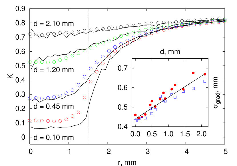
Fig. 1: Contrast $K$ as a function of distance $r$ from the center of the inclusion for different depths $d$. Curves represent simulation results, symbols - experimental results. Vertical line shows the inclusion boundary. Inset: Measured width of the liquid solid-boundary as a function of depth ( $\medbullet$ - simulation data, $\square$ - experiment, line is a guide for the eye).

For the Monte-Carlo simulation we followed the photon packet approach of light propagation in a turbid medium [7]. The Henyey-Greenstein phase function was used based on an average scattering angle $\langle\cos\theta\rangle$ [7]. The degree of polarization was assumed to decay exponentially[8]. The reflections and refractions on the boundaries were treated according to Fresnel formulas. As the refractive index of the Teflon ($n=1.35$) is very close to water ($n=1.33$) interactions with boundaries of dynamic inclusion were not considered. The photon packets back-reflected from the sample where registered within a numerical aperture $0.17$. Only depolarized photons were registered to match the experimental conditions. The field auto-correlation function (ACF) $g_{1}(\tau)$ of the scattered light was determined from the photon packet history as explained in Ref. 9.

In order to quantify the effect of image blurring caused by multiple scattering we determine the standard deviation of the contrast gradient $\sigma_{grad}$ . As can be seen in Fig. 1 starting from the smallest depths the apparent width is increased. This increase is of the order of a few $l^{*}$, which is the relevant length scale for an incident photon to propagate laterally. The smearing increases with depth until for large depths the width becomes of the order of the depth, as expected for diffuse light propagation [10]. Our results show the importance of diffuse blurring in the image formation already for small and moderate depths and can thus provide important guidelines for the analysis of actual experiments in biomedical imaging [3, 4, 5].

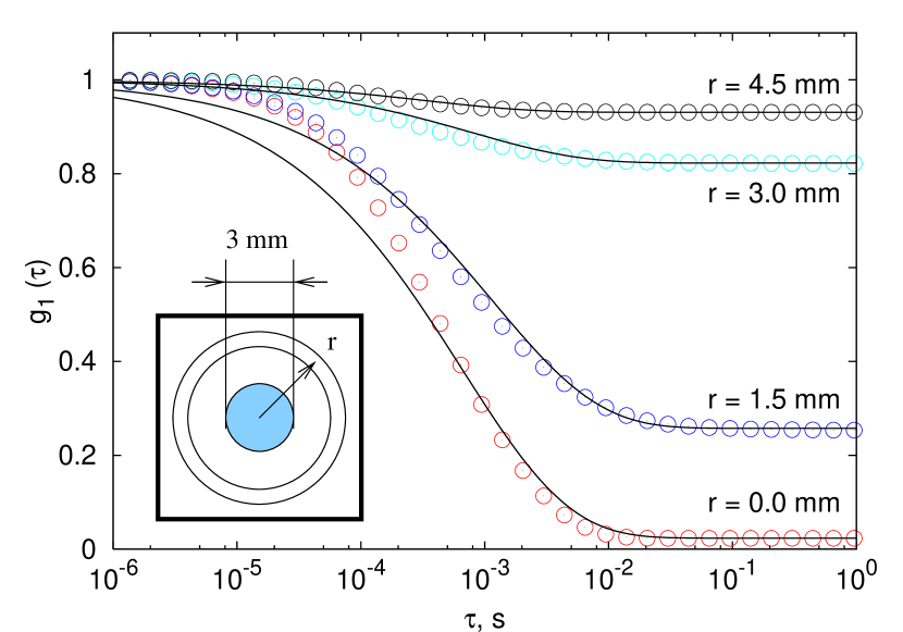
Fig. 2: Simulated correlation functions $g_{1}(\tau)$ for the inclusion depth $d$ = 100 $\mu m$. Solid lines show the fits with DWS theory with baseline. The relaxation times $\tau_{0}$ for the fits were obtained by the contrast $K$ inversion (see Fig. 3).

A typical set of simulated correlation functions is presented in the Fig.2. If $g_{1}(\tau)$ is known, then the speckle contrast $K$ of the time-integrated speckle fluctuations can be obtained via the following relation [11, 12]

$$K^{2}=\frac{\langle I^{2}\rangle}{\langle I\rangle^{2}}-1=\frac{2\beta}{T}\int_{0}^{T}|g_{1}(\tau)|^{2}\left(1-\tau/T\right)d\tau,$$ (1)

where $T$ is the integration time of the detector and $\beta$ the coherence factor of the detection optics. It is important to note that this equation is different to the traditionally used expression of Fercher and Briers [1]. As reaffirmed by Durian and coworkers the correct expression, eq. (1), has to take into account the effect of triangular averaging of the correlation function [11]. As shown in Fig. 1 the resulting values of the contrast are found in quantitative agreement with the experimental data without any adjustable parameter.

A comparison of Fig. 1 and Fig. 2 immediately reveals the main limitation of LSI. A single contrast value $K$ is recorded in practice as compared to the complex correlation function characterizing the full spectrum of intensity fluctuations and thus particular care has to be taken which and how information can be extracted.

In our work we have access to both $K$ and $g_{1}(t)$ and thus we are able to analyze the LSI detection process quantitatively. We first analyze the characteristic features of the correlation functions presented in Fig. 2. Overall the functions are well described by the usual stretched-exponential form derived for diffusing-wave spectroscopy (DWS) of a colloid suspension: $g_{1}(\tau)=\exp(-\gamma\sqrt{6\tau/\tau_{0}})$, where in our case relaxation time $\tau_{0}=1/Dk_{0}^{2}$ characterizes Brownian motion (diffusion coefficient $D$) and $\gamma\approx 2$ is a constant[13, 14]. It is worthwhile to note that for the case of blood flow the relaxation time $\tau_{0}$ is inversely proportional to the root mean square of the flow velocity .

The presence of a non-fluctuating static scattering part, however, leads to a non-zero baseline. Since the relative amount of the static light scattering increases with the distance $r$ from the center, the plateau of the ACF increases as well. It has been noted previously that a non-zero baseline significantly influences or even dominates the resulting values of the contrast $K$ [1]. Nevertheless it is rather common in the biomedical community to convert the obtained contrast values directly to relaxation times neglecting contributions of static scattering [2, 15, 5, 16, 4, 17].

If the detected light is composed of dynamic and static components: $E(t)=E_{d}(t)+E_{s}(t)$ the measured field correlation function is defined as following [18]:

$$g_{1}(\tau)=\rho\left|g_{\textrm{1 d}}\left(\tau\right)\right|+\left(1-\rho\right),$$ (2)

where $\rho=\langle I_{d}\rangle/(\langle I_{d}\rangle+\langle I_{s}\rangle)$ characterizes the fluctuating part of the detected light intensity and $g_{\textrm{1 d}}\left(\tau\right)$ is the field correlation function of the dynamic component. The resulting contrast value can be calculated by substituting eq. (2) into eq. (1):

$$K_{m}^{2} = \frac{2\beta}{T}\int_{0}^{T}\left[\rho\left|g_{1d}\left(\tau\right)\right|+\left(1-\rho\right)\right]^{2}\left(1-\tau/T\right)d\tau$$ (3)

$$= \beta\left[\rho^{2}K^{2}_{2\>d}+2\rho\left(1-\rho\right)K_{1\>d}^{2}+\left(1-\rho\right)^{2}\right],$$

where $K^{2}_{\textrm{2 d}}=1/T\int_{0}^{T}\left|g_{\textrm{1 d}}\left(\tau\right)\right|^{2}\left(1-\tau/T\right)d\tau$ and $K^{2}_{\textrm{1 d}}=1/T\int_{0}^{T}\left|g_{\textrm{1 d}}\left(\tau\right)\right|\left(1-\tau/T\right)d\tau$ are the normalized variances of the intensity and field fluctuations of the dynamic part of the detected signal with $K_{\textrm{2 d}}<K_{\textrm{1 d}}$. The last term in eq. (3) is time independent and reflects the impact of the static scattering contribution. Thus the contrast $K_{m}$ measured in an LSI experiment is given by the dynamic contrast of intensity fluctuations $K_{\textrm{2 d}}$, the dynamic contrast of the field fluctuations $K_{\textrm{1 d}}$ and $\rho$.

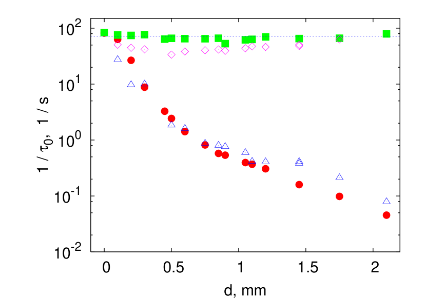
Fig. 3: Inverse of the relaxation time $1/\tau_{0}$ as a function of depth obtained by directly converting the contrast $K$ based on Eq.1 neglecting the static part: $\medbullet$ - simulation data, $\bigtriangleup$ - experiment and using the correct procedure based on Eq. 3: $\blacksquare$ - simulation and $\Diamond$ - experiment. Horizontal dashed line - actual value of the relaxation time.

In an actual LSI experiment an additional processing step has to be introduced in order to separate the dynamic and static part. The camera exposure time $T$ is usually larger compared to the relaxation time $\tau_{0}$ related to blood flow and subsequent frames are separated by a period $\Delta t$ larger than $T$. Since $\Delta t>T>\tau_{0}$ two sequential frames are free of the dynamic component of interest and thus the time and space dependent static or pseudo-static component can be easily found by cross-correlating sequential frames $\rho\left(t,{\bf r}\right)=1-\left[\langle I\left(t,{\bf r}\right)I\left(t+\Delta t,{\bf r}\right)\rangle_{s}/\langle I\left(t,{\bf r}\right)\rangle_{s}^{2}-1\right]^{1/2}$.

Fig. 3 shows a comparison of the correct inversion procedure based on eq. (3) as compared to the one neglecting static scattering [12]. While the correct procedure produces values comparable to the relaxation time of Brownian motion $\tau_{0}$ the direct conversion can deviate by several orders of magnitude.

In conclusion, we studied the image blurring of an object buried in turbid media and found that the resolution of the obtained images can be affected significantly by multiple scattering. We furthermore introduced a model that reflects the impact of the static scattering on the quantitative interpretation of LSI images. A simple procedure has been suggested to perform a quantitative analysis in actual LSI experiments.

Financial support from the Swiss National Science foundation is gratefully acknowledged. Correspondence should be addressed to Frank Scheffold (e-mail, Frank.Scheffold@unifr.ch) or Pavel Zakharov (e-mail, Pavel.Zakharov@unifr.ch)

References

- [1] J. D. Briers. Laser doppler, speckle and related techniques for blood perfusion mapping and imaging. Physiological Measurement, 22(4):R35–R66, 2001.
- [2] A. K. Dunn, H. Bolay, M. A. Moskowitz, and D. A. Boas. Dynamic imaging of cerebral blood flow using laser speckle. J. Cereb. Blood Flow Metab., 21:195 – 201, 2001.
- [3] B. Weber, C. Burger, M. T. Wyss, G. K. von Schulthess, F. Scheffold, and A. Buck. Optical imaging of the spatiotemporal dynamics of cerebral blood flow and oxidative metabolism in the rat barrel cortex. Eur J Neurosci, 20(10):2664, 2004.
- [4] T. Durduran, M. G. Burnett, C. Zhou G. Yu, D. Furuya, A. G. Yodh, J. A. Detre, and J. H. Greenberg. Spatiotemporal quantification of cerebral blood flow during functional activation in rat somatosensory cortex using laser-speckle flowmetry. Journal of Cerebral Blood Flow & Metabolism, 24:518–525, 2004.
- [5] A.K. Dunn, A. Devor, A.M. Dale, and D.A. Boas. Spatial extent of oxygen metabolism and hemodynamic changes during functional activation of the rat somatosensory cortex. NeuroImage, 27(15):279 – 290, 2005.
- [6] A.C. Völker, P. Zakharov, B. Weber, F. Buck, and F. Scheffold. Laser speckle imaging with active noise reduction scheme. Opt. Exp., 13(24):9782 – 9787, 2005.
- [7] S. A. Prahl, M. Keijzer, S. L. Jacques, and A. J. Welch. A monte carlo model of light propagation in tissue. In G. J. Müller and D. H. Sliney, editors, SPIE Proceedings of Dosimetry of Laser Radiation in Medicine and Biology, volume IS 5, pages 102 – 111, 1989.
- [8] D. A. Zimnyakov. On some manifestations of similarity in multiple scattering of coherent light. Waves Random Media, 10:417 – 434, 2000.
- [9] D.J. Durian. Accuracy of diffusing-wave spectroscopy theories. Phys. Rev. E , 51:3350 – 3358, 1995.
- [10] M. Heckmeier and G. Maret. Dark speckle imaging of colloidal suspensions in multiple light scattering media. PROGRESS IN COLLOID AND POLYMER SCIENCE, 104:12 – 16, 1997.
- [11] K Schätzel. Noise on photon correlation data. i. autocorrelation functions. Quantum Optics: Journal of the European Optical Society Part B, 2(4):287–305, 1990.
- [12] R. Bandyopadhyay, A.S. Gittings, S.S. Suh, P.K. Dixon, and D.J. Durian. Speckle-visibility spectroscopy: A tool to study time-varying dynamics. Rev. Sci. Instrum., 76:093110, 2005.
- [13] B.J. Berne and R. Pecora. Dynamic Light Scattering. With Applications to Chemistry, Biology, and Physics. Dover Publications, Inc., New York, 2000.
- [14] D.J. Pine, D.A. Weitz, P.M. Chaikin, and E. Herbolzheimer. Diffusing-wave spectroscopy. Phys. Rev. Lett. , 60:1134–1137, 1988.
- [15] A. Dunn, A. Devor, M. Andermann, H. Bolay, M. Moskowitz, A. Dale, and D. Boas. Simultaneous imaging of total cerebral hemoglobin concentration, oxygenation and blood flow during functional activation. Optics Letters, 28:28 – 30, 2003.
- [16] S. Yuan, D.A. Boas, and A.K. Dunn. Determination of optimal exposure time for imaging of blood flow changes with laser speckle contrast imaging. Appl. Opt. , 2005.
- [17] Haiying Cheng, Qingming Luo, Qian Liu, Qiang Lu, Hui Gong, and Shaoqun Zeng. Laser speckle imaging of blood flow in microcirculation. Physics in Medicine and Biology, 49(7):1347–1357, 2004.
- [18] D. A. Boas and A. G. Yodh. Spatially varying dynamical properties of turbid media probed with diffusing temporal light correlation. JOSA, 14(1):192 – 215, 1997.