Multiple crossovers in interacting quantum wires

Abstract

We study tunneling of electrons into and between interacting wires in the spin-incoherent regime subject to a magnetic field. The tunneling currents follow power laws of the applied voltage with exponents that depend on whether the electron spins at the relevant length scales are polarized or disordered. The crossover length (or energy) scale is exponential in the applied field. In a finite size wire multiple crossovers can occur.

I Introduction

The Luttinger Liquid is considered to be the appropriate description of the low-energy properties of interacting electrons in a quantum wire.Haldane (1981); Giamarchi (2004) In a Luttinger Liquid, the fundamental excitations are collective charge and spin modes. Unlike Fermi Liquids, Luttinger Liquids have power law dependences for the tunneling density of states and for the conductance through a weak link as a function of the applied bias voltage or temperature. This and other properties of Luttinger Liquids such as the phenomenon of spin-charge separation have been observed experimentally. Yao et al. (1999); Bockrath et al. (1999); Auslaender et al. (2002); Ishii et al. (2003)

Recently, it has been realized that the electron liquid with spin excitation energy $J$ smaller than the temperature $T$ differs qualitatively from the standard Luttinger Liquid picture.Cheianov and Zvonarev (2004a, b); Cheianov et al. (2005); Matveev (2004a, b); Fiete and Balents (2004); Fiete et al. (2005a, b, 2006); Kindermann and Brouwer (2005); Kindermann et al. (2006); Kakashvili and Johannesson (2006); Fiete (2005); Matveev et al. (2006) This ‘spin-incoherent’ limit can be realized in quantum wires at low densities, when the conductor enters the Wigner crystal regime and $J$ is exponentially suppressed below the Fermi energy $E_{F}$ by the Coulomb barrier between adjacent electrons in the crystal.Klironomos et al. (2005); Fogler and Pivovarov (2005) Recent experiments on wires defined in heterostructures approach this regime.Auslaender et al. (2002); Fiete et al. (2005a) The spin-incoherent limit can also be reached in ultra-thin quantum wires, in which the Coulomb repulsion renders the electrons effectively impenetrable.Fogler (2005) A theoretical model that shows spin-incoherence is the one-dimensional Hubbard model with infinite on-site repulsion $U$.

The qualitative difference between the cases $J=0$ and $J\neq 0$ arises because for $J=0$ the velocity $v_{s}$ of spin excitations is zero. This implies that the relative positions of the electron spins are fixed if $J=0$. Their absolute positions along the wire, however, are not. Spin can still move along the wire together with the flow of charge. This is best visualized in the infinite-$U$ Hubbard model, which has an exact solution in terms of a static spin background and non-interacting spinless holes, which are the charge carriers,Bernasconi et al. (1975) see Fig. 1. The same coupling between spin and charge generically exists also in Luttinger Liquids with $J\neq 0$, but its impact on the low-energy properties is overwhelmed by the effects of the finite spin velocity in the standard case. For spin-incoherent Luttinger Liquids, the motion of the spin background driven by quantum fluctuations of the charge current has been shown to give rise to an anomalous dependence of the tunneling current $I$ through a probe weakly coupled to the quantum wire on the applied voltage $V$. This occurs because the spin background at the point of tunneling is not static on the time scale $\simeq\hbar/eV$ of a tunneling event. In Refs. Cheianov and Zvonarev, 2004a; Fiete and Balents, 2004 it was shown that foo

$$I\propto V^{1/2}$$ (1)

if there are no residual interactions between the charge degrees of freedom, whereas $I\propto V$ in the $J\downarrow 0$ limit of finite-$J$ Luttinger Liquids in the same situation.

Figure 1: Hubbard chain with infinite on-site repulsion $U$ that allows sites to be singly occupied only. a) Moving charge carriers (holes in the electron occupation) shift also the spin configuration such that the spin state at a given site may change. The relative position of the spins remains fixed, however. b) The spin state at a given site does not fluctuate in a spin-polarized Hubbard chain, when the spin configuration is translationally invariant. c) Also the spin configuration at the site that is at the end of the chain cannot be changed by the charge dynamics.

The motion of the spin background has no effect on the tunneling current if a magnetic field $B$ is applied large enough to polarize the electron spins in the quantum wire and in the probe. In that case, the spin background is translation invariant and one restores the dependence $I\propto V$ of the non-interacting case. The tunneling current of minority electrons remains anomalous, however, since the addition of minority electrons to the quantum wire always breaks the translation invariance of the wire’s spin background.

A second possibility to restore the noninteracting tunneling exponent in a spin-incoherent Luttinger Liquid is to move the tunneling probe to the end of the wire. In that case there is no room for variation of the positions of the spins in the wire relative to the point of tunneling. The spin of an electron tunneling into the wire is simply added to the end of the spin configuration in the wire prior to tunneling.

In this article we ask the question how the crossover between the different tunneling exponents takes place. For both crossovers — as a function of applied magnetic field or as a function of the distance from the end of the wire — we find that the dependence $I\propto V^{\alpha}$ of the tunneling current on the applied voltage switches between two different exponents $\alpha$. For the magnetic-field induced crossover, we find that the majority-electron current $I\propto V^{1/2}$ for $V\ll V_{B}$, whereas $I\propto V$ for higher bias voltages, where the crossover voltage $V_{B}$ can be found as the lowest voltage at which the $(E_{F}/eV)^{1/2}$ spins bordering the tunneling site can still be expected to be majority spins,

$$eV_{B}=E_{F}e^{-2E_{\rm Z}/k_{B}T}.$$ (2)

Here $E_{\rm Z}=2\mu_{B}B$, where $\mu_{B}$ is the Bohr magneton, is the Zeeman energy of electrons in the applied magnetic field $B$. For the crossover that depends on the distance $x$ from the wire’s end, one has $I\propto V$ for $V\ll V_{x}$, with

$$V_{x}=\hbar v/x,$$ (3)

whereas $I\propto V^{1/2}$ for higher bias voltages, where $v$ is the velocity of the collective charge modes in the quantum wire.

Our detailed calculations are described in the remainder of this article. In Sec. II we discuss the bosonized description of a one-dimensional conductor in the spin-incoherent limit. In Sec. III we present a detailed calculation of the single-electron Green functions of the one-dimensional wire. Finally, in Sec. IV we discuss the consequences that the asymptotic time-dependence of the Green functions has for tunneling experiments. In our calculations, we take into account that there may exist additional forward scattering interactions between the charge excitations. This applies, for instance, to a quantum wire at low electron densities when the wire enters the Wigner crystal regime. The charge dynamics in such a quantum wire is described by a spinless Luttinger Liquid with interaction parameter $g$.Fiete and Balents (2004); Fiete et al. (2005b) The tunneling exponents listed above are for the case $g=1$. For general $g$ the nature of the crossovers is unchanged, although the estimates of the crossover voltages and the exact tunneling exponents are modified.

II Model

At low energies an interacting wire in the spin-incoherent regime is described by a spinless charge degree of freedom and a static spin background. Fiete and Balents (2004) The spin background does not enter the Hamiltonian. We describe the charge degree of freedom using boson fields $\theta$ and $\phi$, which are related to the charge density $\rho$ through

$$\rho=\frac{e}{\pi}\frac{\partial\theta}{\partial x}.$$ (4)

We consider a half-infinite quantum wire $0<x<\infty$. For a half-infinite wire, the boson fields have the commutation relation

$$[\theta(x),\phi(x^{\prime})]=-i\pi\Theta(x-x^{\prime}),$$ (5)

where $\Theta(y)=1$ if $y>0$ and $0$ otherwise, and satisfy the boundary condition $\theta(x)=0$ and $\partial\phi(x)/\partial x=0$ at $x=0$. The Hamiltonian is

$$H=v\int_{0}^{\infty}{\frac{dx}{2\pi}\left[g^{-1}(\partial_{x}\theta)^{2}+g(\partial_{x}\phi)^{2}\right]},$$ (6)

where $g$ sets the strength of the residual interactions between the charge excitations and $v$ is the velocity of the charge carriers. One has $g<1$ for repulsive interactions (we set $\hbar=1$).

The annihilation operator $\psi_{\sigma}(x)$ of an electron with spin $\sigma$ at position $x$ is expressed in terms of spinless fermions $c(x)$ and operators $S_{\sigma}(x)$ that remove a spin $\sigma$ from the spin background of the wire at position $x$ as

$$\psi_{\sigma}(x)=c^{\dagger}(x)S_{\sigma}(x).$$ (7)

The annihilation operator $c$ for the spinless charge carrier is expressed in terms of the boson fields as

$$c(x) = \frac{\eta}{\sqrt{2\pi a}}$$

$$\mbox{}\times\left[e^{-ik_{F}x-i\theta(x)+i\phi(x)}+e^{ik_{F}x+i\theta(x)+i\phi(x)}\right].$$

Here $\eta$ is a Majorana fermion, $k_{F}$ is the Fermi wavenumber of the spinless charge carriers, and $a$ the short-distance cut-off of the bosonized theory.

In the calculations below we need the correlation functions of the boson fields at zero temperature. Up to a (divergent) constant that disappears from the final results, these areFabrizio and Gogolin (1995)

$$-i\langle\phi(x,\tau)\theta(x,0)\rangle = \frac{i}{4}\sum_{\pm}(\mp)\ln[a+i(v\tau\pm 2x)],$$

$$-i\langle\theta(x,\tau)\phi(x,0)\rangle = \frac{i}{4}\sum_{\pm}(\pm)\ln[a+i(v\tau\pm 2x)],$$

$$-i\langle\phi(x,\tau)\phi(x,0)\rangle = \frac{i}{2g}\ln(a+iv\tau)$$

$$\mbox{}+\frac{i}{4g}\sum_{\pm}\ln(a+i(v\tau\pm 2x)),$$

$$-i\langle\theta(x,\tau)\theta(x,0)\rangle = \frac{ig}{2}\ln(a+iv\tau)$$

$$\mbox{}-\frac{ig}{4}\sum_{\pm}\ln(a+i(v\tau\pm 2x)).$$

The Hamiltonian (6) can be derived microscopically as the low-energy theory of a Hubbard model with infinite interaction parameter $U$ and additional long-range interactions described by a purely forward scattering density-density interaction. For this derivation, one describes the infinite-$U$ Hubbard model in terms of a static spin background and spinless holes. The latter are the fermions $c$ introduced above.Ogata and Shiba (1990); Kindermann and Brouwer (2005) At low energies one may linearize the spectrum of the holes, writing the annihilation operator of a hole as $c(x)=e^{ik_{F}x}c_{L}(x)+e^{-ik_{F}x}c_{R}(x)$. Including the long-range interactions between the hole densities $\rho_{L}(x)=c^{\dagger}_{L}(x)c^{\phantom{\dagger}}_{L}(x)$ and $\rho_{R}(x)=c^{\dagger}_{R}(x)c^{\phantom{\dagger}}_{R}(x)$, we then find a Hamiltonian of the form

$$H = \int_{0}^{\infty}dx\left\{-iv_{F}(c^{\dagger}_{L}\partial_{x}c^{\phantom{\dagger}}_{L}-c^{\dagger}_{R}\partial_{x}c^{\phantom{\dagger}}_{R})\right.$$

$$\left.\mbox{}+\frac{g_{0}}{2}\left[\rho_{L}^{2}(x)+\rho_{R}^{2}(x)\right]+\tilde{g}_{0}\rho_{L}(x)\rho_{R}(x)\right\}.$$

This Hamiltonian is brought into the form of Eq. (6) by bosonization of the operators $c_{L}$ and $c_{R}$. The phenomenological parameters $v$ and $g$ in Eq. (6) are related to those in Eq. (II) by $v=v_{R}[(1+g_{0}/2\pi v_{F})^{2}-(\tilde{g}_{0}/2\pi v_{F})^{2}]^{1/2}$ and $g=(1+g_{0}/2\pi v_{F}-\tilde{g}_{0}/2\pi v_{F})^{1/2}/(1+g_{0}/2\pi v_{F}+\tilde{g}_{0}/2\pi v_{F})^{1/2}$. The hole operators $c$ take the form of Eq. (II) after bosonization.

III Calculation

In order to compute the tunneling current $I$ from a tunneling probe into the wire at a distance $x$ from the wire’s end, we express $I$ in terms of the Green functions $G$ and $G_{\rm p}$ of the wire and the probe, respectively. To lowest order in the tunneling amplitude $t$ between wire and probe one has

$$I = 2|t|^{2}\sum_{\sigma}\int d\tau\,e^{-ieV\tau/\hbar}$$

$$\mbox{}\times\left[G^{<}_{\sigma}(x,\tau)G^{>}_{{\rm p},\sigma}(x,-\tau)-G^{>}_{\sigma}(x,\tau)G^{<}_{{\rm p},\sigma}(x,-\tau)\right].$$

The greater and lesser Green functions of the wire are defined as

$$G_{\sigma}^{>}(x,\tau) = -i\langle\psi^{\phantom{\dagger}}_{\sigma}(x,\tau)\psi^{\dagger}_{\sigma}(x,0)\rangle,$$

$$G_{\sigma}^{<}(x,\tau) = i\langle\psi^{\dagger}_{\sigma}(x,0)\psi^{\phantom{\dagger}}_{\sigma}(x,\tau)\rangle,$$ (12)

with similar definitions for the greater and lesser Green functions of the probe.

The power-law dependence of the tunneling current $I$ on the applied voltage $V$ at low $V$ is related to the time-dependence of the wire Green functions at large $\tau\simeq\hbar/eV$. In terms of hole and spin operators we have

$$G_{\sigma}^{>}(x,\tau)=-i\langle S^{\phantom{\dagger}}_{\sigma}(x,\tau)c^{\dagger}(x,\tau)c(x,0)S^{\dagger}_{\sigma}(x,0)\rangle.$$ (13)

The spin expectation value in Eq. (13) is non-vanishing only if all background spins between the spin that is at position $x$ at time $\tau$ and the spin that is at $x^{\prime}$ at time $0$ have the same orientation $\sigma$. This occurs with probability $p_{\sigma}^{|N_{x}(\tau)-N_{x}(0)|}$, where

$$N_{x}(\tau)=\frac{k_{F}x+\theta(x,\tau)}{\pi}$$ (14)

is the number of electrons between positions $0$ and $x$ at time $\tau$ and

$$p_{\uparrow}=1-p_{\downarrow}=\frac{1}{e^{-E_{\rm Z}/k_{B}T}+1}$$ (15)

is the probability for a spin to point along the direction of the applied magnetic field. One then evaluates the greater Green function asFiete and Balents (2004); Fiete et al. (2005a)

$$G_{\sigma}^{>}(x,\tau) = -ie^{iE_{\rm Z}\sigma\tau/2}\sum_{k}p_{\sigma}^{|k|}\int\frac{d\xi}{2\pi}\,e^{i\xi k}$$

$$\mbox{}\times\langle e^{-i\xi N_{x}(\tau)}c^{\dagger}(x,\tau)c(x,0)e^{i\xi N_{x}(0)}\rangle.$$

Here, $\sigma$ equals $1$ for spin-up electrons and $-1$ for spin-down electrons. Using the correlators of Eq. (II), we then find

$$G_{\sigma}^{>}(x,\tau) \propto e^{iE_{\rm Z}\sigma\tau/2}\sum_{k}\,\frac{p_{\sigma}^{|k|}e^{-k^{2}/2w^{2}}}{2\pi wa}\left\{2(-1)^{k}\left[\frac{4x^{2}a^{2}}{\left((iv\tau+a)^{2}+4x^{2}\right)(iv\tau+a)^{2}}\right]^{1/4g}\right.$$ (17)

$$\left.\mbox{}+\frac{(iv\tau+a)^{g/2-1/2g}a^{g/2+1/2g}}{(2x)^{g/2-1/2g}((iv\tau+a)^{2}+4x^{2})^{(g-1)^{2}/4g}}\left(\frac{e^{2ik_{F}x}}{iv\tau-2ix+a}+\frac{e^{-2ik_{F}x}}{iv\tau+2ix+a}\right)\right\}$$

with

$$w^{2}=-\frac{g}{2\pi^{2}}\ln\left[\frac{a^{2}}{4x^{2}}+\frac{a^{2}}{(iv\tau+a)^{2}}\right].$$ (18)

The symbol “$\propto$” in Eq. (17) indicates dimensionless prefactors that do not depend on $\tau$, $x$, or $p_{\sigma}$. For the Green functions needed in this article the lesser functions $G^{<}(x,\tau)$ are obtained by the replacement

$$G_{\sigma}^{<}(x,\tau)=p_{\sigma}e^{iE_{\rm Z}\sigma\tau}G_{\sigma}^{>}(x,\tau)^{*}|_{k_{F}\leftrightarrow-k_{F}}.$$ (19)

The extra factor $p_{\sigma}$ originates from the reversed order of the spin operators $S(x,\tau)$ and $S^{\dagger}(x,\tau)$ in the expression for $G^{<}(x,\tau)$.

We should note that our calculation using bosonization is not exact since it does not account for the discreteness of charge. For this reason, the sum over $k$ was replaced by an integral in Ref. Kindermann et al., 2006. With this replacement, the Green functions at non-coinciding points agree with the exact Green functions in the limit $p_{\sigma}\to 1$. None of the Green functions at coinciding points considered in this article depends on whether one has a sum or an integral in this limit. We therefore keep the sums, which results in improved approximations in the opposite limit $p_{\sigma}\to 0$.

The sum over $k$ in Eq. (17) is time- and space-dependent through $w$. In previous treatments of the problem in Refs. Fiete and Balents, 2004; Fiete et al., 2005a; Kindermann et al., 2006 this dependence has been neglected. This is a good approximation for an unpolarized electron gas at not too large energies. As one polarizes the electron spins by applying a magnetic field, however, this additional time and space-dependence in Eq. (17) becomes more and more important and we will show that it leads to the expected crossover of the scaling exponent to the conventional Luttinger Liquid exponent at perfect spin-polarization.

III.1 Crossover induced by a magnetic field

To evaluate Eq. (17) we need the sum

$$S=\sum_{k}\,(-1)^{k}p^{|k|}e^{-k^{2}/2w^{2}}$$ (20)

with $0\leq p\leq 1$. Using the identity

$$\sum_{k}f(k)=\int dk\,f(k)\sum_{q}e^{2i\pi qk},$$

we first convert the sum over $k$ into an integral,

$$S=2\sum_{q}\int_{0}^{\infty}dk\,e^{-i\pi(2q+1)k+k\ln p-k^{2}/2w^{2}}.$$ (21)

Although this integral can be expressed in terms of error functions, the power-law dependence on $\tau$ can be extracted using a sequence of approximations. For this we confine ourselves to the regime $\pi|w|\gg 1$, which is appropriate in the relevant case that the distance from the end of the wire is not microscopic ($x\gg a$) and the time $\tau$ is large. We first rewrite $S$ by shifting the contour of integration in the complex plane,

$$S=S_{1}+S_{2},$$ (22)

with

$$S_{1} = -2i\sum_{q}e^{-\pi^{2}w^{2}(2q+1)^{2}/2}\int_{0}^{\pi w^{2}(2q+1)}d\kappa\,e^{\kappa^{2}/2w^{2}}$$

$$\mbox{}\times e^{i\ln p\left(\kappa-\pi w^{2}(2q+1)\right)},$$

$$S_{2} = 2\sum_{q}e^{w^{2}[\ln p-i\pi(2q+1)]^{2}/2}\int_{w^{2}|\ln p|}^{\infty}dk\,e^{-k^{2}/2w^{2}}.$$

At $\pi|w|\gg 1$ the $\kappa$ integration in $S_{1}$ is dominated by $\kappa$ close to $\pi w^{2}(2q+1)$. Linearizing the exponent around $\kappa=\pi w^{2}(2q+1)$, we then find

$$S_{1} \approx -\sum_{q}\frac{2}{\ln p-i\pi(2q+1)}$$ (23)

$$= \frac{1-p}{1+p}.$$

Each term in the $q$-summation for $S_{2}$ can be bounded by $e^{-\pi^{2}(2q+1)^{2}w^{2}/2}/|\ln p|$, from which one concludes that $S_{1}$ dominates over $S_{2}$ unless $|\ln p|\lesssim\exp(-\pi^{2}w^{2}/4)$. Since $\exp(-\pi^{2}w^{2}/4)\ll 1/w^{2}$, one may in our limit $\pi w\gg 1$ thus calculate $S_{2}$ in the limit $\ln p\to 0$. We then find

$$S\approx\frac{1-p}{1+p}+\sqrt{2\pi}w\,e^{-w^{2}\pi^{2}/2}$$ (24)

in the regime of interest $\pi|w|\gg 1$. The numerical comparison shown in Fig. 2 shows that Eq. (24) is indeed an excellent approximation to the sum Eq. (20).

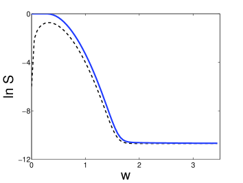
Figure 2: Comparison between the logarithms of the sum $S$ (solid line) and its approximation Eq. (24) (dashed line) at $E_{\rm Z}=10\,k_{B}T$. The approximation improves as $w$ grows large.

In order to study the magnetic-field dependence of tunneling into the bulk of a spin-incoherent wire, we take $v\tau\ll x$ in Eq. (17). Using Eq. (24), we then find

$$G_{\sigma}^{>}(\tau) \propto \frac{e^{iE_{\rm Z}\sigma\tau/2}}{a}\Bigg{[}\frac{1}{\sqrt{2\pi}w}\frac{1-p_{\sigma}}{1+p_{\sigma}}\left(\frac{a}{iv\tau+a}\right)^{1/2g}\$$ (25)

$$\mbox{}+\left(\frac{a}{iv\tau+a}\right)^{g/2+1/2g}\Bigg{]}.$$

The first term has the anomalous scaling $\propto\tau^{-1/2g}$ calculated in Refs. Cheianov and Zvonarev, 2004a; Fiete and Balents, 2004 for the spin-incoherent Luttinger Liquid at zero magnetic field. (We neglect the logarithmic time dependence following from the prefactor $w$ in Eq. (25).) The second term has the asymptotic time-dependence characteristic of a standard Luttinger Liquid at interaction parameter $g$. In the absence of a magnetic field, the first term dominates. In the presence of a magnetic field that partially polarizes the electron spins, the first term remains dominant for minority electrons. For majority electrons, however, there is a range of times $\tau\ll\tau_{B}$ in which the second term takes over, with

$$\tau_{B}=\frac{a}{v}e^{2E_{\rm Z}/gk_{B}T}.$$ (26)

Hence, for times $\tau\ll\tau_{\rm B}$, $G^{>}\propto\tau^{-1/2g-g/2}$, whereas $G^{>}\propto\tau^{-1/2g}$ for $\tau\gg\tau_{\rm B}$. Qualitatively, the crossover occurs when the electrons have a sufficiently long time $\tau_{B}$ to explore distances over which the electron spins are disordered. With increasing polarization that time increases. Note that the range $\tau\ll\tau_{\rm B}$ is observable only if $\tau_{\rm B}\gg a/v$, which requires polarizations $p_{\uparrow}$ close to unity. Conversely, at any given $\tau$ (corresponding to a fixed bias voltage $V$) the tunneling current of majority spin electrons displays a strong magnetic field dependence: the dependence is exponential $\exp(-E_{\rm Z}/k_{B}T)$ for $E^{*}_{\rm Z}\gtrsim E_{\rm Z}\gg k_{B}T$ and saturates in fields larger than the crossover field $B^{*}$ with

$$E_{Z}^{*}=\frac{g}{2}k_{B}T\ln\frac{v\tau}{a}.$$ (27)

III.2 Crossover as a function of distance from a boundary

The anomalous scaling of spin-incoherent electrons can not only be suppressed by polarizing the spins, but also by moving the tunneling probe toward the end of the wire. Close to the end of the wire, the sliding of the spin background is suppressed, and one expects to recover the standard tunneling exponents for times $\tau\gg\tau_{x}\equiv x/v$. For $\tau\gg\tau_{\rm B}$ (when the conductor exhibits an anomalous exponent for tunneling into the bulk) we find

$$G_{\sigma}^{>}(\tau) \propto \frac{e^{iE_{\rm Z}\sigma\tau/2}}{wa}\frac{1-p_{\sigma}}{1+p_{\sigma}}$$

$$\mbox{}\times\left[\frac{4x^{2}a^{2}}{\left((iv\tau+a)^{2}+4x^{2}\right)(iv\tau+a)^{2}}\right]^{1/4g}.$$

Note that one indeed recovers the behavior $G^{>}(\tau)\propto\tau^{-1/g}$ for tunneling near the end of a standard Luttinger Liquid if $\tau\gg\tau_{x}$.

In the regime $\tau_{B}\ll\tau_{x}$ one expects a double crossover for majority electrons: For very small times $\tau\ll\tau_{B}$, one observes the exponent characteristic of a fully polarized electron gas, $G^{>}(\tau)\propto\tau^{-1/2g-g/2}$. For the intermediate range $\tau_{B}\ll\tau\ll\tau_{x}$, tunneling shows the anomalous exponent characteristic of the bulk spin-incoherent Luttinger Liquid, $G^{>}(\tau)\propto\tau^{-1/2g}$. The true asymptotic behavior sets in only for $\tau\gg\tau_{x}$ and shows the power-law dependence $G^{>}\propto\tau^{-1/g}$ for to-end tunneling of a standard Luttinger Liquid. Both crossovers can be inferred from the form of the Green function at $\pi|w|\gg 1$ that is obtained by substituting Eq. (24) into Eq. (17) without taking any further limits,

$$G_{\sigma}^{>}(x,x,\tau) \propto e^{iE_{\rm Z}\sigma\tau/2}\left[\frac{4x^{2}a^{2}}{\left((iv\tau+a)^{2}+4x^{2}\right)(iv\tau+a)^{2}}\right]^{1/4g}\left\{\frac{\sqrt{2}}{\sqrt{\pi}w}\,\frac{1-p_{\sigma}}{1+p_{\sigma}}+\left[\frac{a^{2}\left((iv\tau+a)^{2}+4x^{2}\right)(iv\tau+a)^{2}}{4x^{2}}\right]^{g/4}\right.$$ (29)

$$\mbox{}\left.\times\left[\frac{2}{(iv\tau+a)^{g}}+\frac{1}{\left((iv\tau+a)^{2}+4x^{2}\right)^{(g-1)/2}}\left(\frac{e^{2ik_{F}x}}{iv\tau-2ix+a}+\frac{e^{-2ik_{F}x}}{iv\tau+2ix+a}\right)\right]\right\}.$$

While the first crossover at $\tau\approx\tau_{B}$ is obtained by comparing the magnitudes of the two terms inside the curly brackets, the second one at $\tau\approx\tau_{x}$ is described by the factor outside the curly brackets in Eq. (29).

IV Consequences for tunneling experiments

We now discuss the implications of Eqs. (25), (III.2), and (29) for tunneling experiments. We consider two cases: tunneling from one spin-incoherent wire into another one and tunneling from a noninteracting conductor, such as a metallic STM-tip, into a spin-incoherent wire.

configuration:	end-end	bulk-end	bulk-bulk
$\alpha_{\rm pol}$	$2/g-1$	$3/2g+g/2-1$	$1/g+g-1$
$\alpha_{\rm incoh}$	$2/g-1$	$3/2g-1$	$1/g-1$

Table 1: Scaling exponents for the tunneling currents between two spin-incoherent conductors subject to a magnetic field in various configurations. The spin-polarized exponents $\alpha_{\rm pol}$ govern the tunneling current at high voltages. The crossovers between them and the incoherent exponents $\alpha_{\rm incoh}$ occur at the voltage scales $eV_{B}=E_{F}\exp(-2E_{\rm Z}/gk_{B}T)$ for tunneling from bulk to end and $eV^{*}_{B}=E_{F}\exp(-E_{\rm Z}/gk_{B}T)$ for bulk to bulk tunneling.

In the first case, there is no real difference between ‘probe’ and ‘wire’. As a result, the exponent $\alpha$ governing the power-law dependence of the tunneling current $I$ on the applied voltage $V$,

$$I\propto V^{\alpha},$$ (30)

depends on whether the tunneling takes place from the bulk or from the end of the probe wire. The various exponents $\alpha_{\rm incoh}$ (characteristic of the spin-incoherent Luttinger Liquid) and $\alpha_{\rm pol}$ (characteristic of the spin-polarized electron liquid) for tunneling from end to end, bulk to end, and bulk to bulk respectively, are summarized in table 1. The crossovers between bulk and end behavior occur at the corresponding scale $V\simeq V_{x}$.

For tunneling from the end of the probe, the density of states in the probe is independent of energy. Hence, the crossovers between various power law exponents for majority spin electrons described by Eqs.  (25) and (29) are observable at the scales derived in sections III.1 and III.2. The magnetic field dependence of the tunneling current in this configuration is given by that of the majority spin Green function derived in section III.1.

For tunneling from the bulk of the probe wire into the bulk of the probed wire the crossover takes place between a regime of high energies where the majority spin current dominates to a low energy regime where the current is carried by minority spin electrons. The fact that the minority spin current dominates at low bias can be seen from the low voltage limit $I_{\sigma}\propto p_{\sigma}(1-p_{\sigma})^{2}$ if $\tau\gg\tau_{B}$. It follows from the long-time asymptote of Eq. (25), used in Eq. (III) together with Eq. (19). The voltage at which the minority and majority spin currents are equal is

$$eV_{B}^{*}\simeq E_{F}e^{-E_{\rm Z}/gk_{B}T}.$$ (31)

At high voltages, $V\gg V_{B}^{*}$, the power law exponent $\alpha$ is that characteristic of a fully polarized wire $\alpha_{\rm pol}$. At low voltages, one observes the exponent of a spin-incoherent wire, $\alpha_{\rm incoh}$, see Tab. 1.

If tunneling takes place from a noninteracting conductor, the phase $\exp(iE_{\rm Z}\sigma\tau/2)$ in the Green function of the spin-incoherent wire becomes important. (This phase factor cancels for tunneling between spin-incoherent conductors.) The phase factor $\exp(iE_{\rm Z}\sigma\tau/2)$ represents the extra energy cost $E_{\rm Z}$ necessary to tunnel minority spin electrons into the spin-incoherent wire. This energy cost appears because, while the higher magnetic energy of the minority electrons is compensated for by a reduction of their kinetic energy in the non-interacting probe, this is not possible in the spin-incoherent conductor, where the holes $c$ have a kinetic energy that is independent of the spin of the missing electron. As a consequence, the chemical potentials of the spinless charge carriers in the spin-incoherent conductor and of the electrons in the probe at zero temperature differ by the amount $E_{\rm Z}/2$, the energy gain $E_{\rm Z}/2$ for adding a majority spin to the wire.

We now assume that $E_{\rm Z}\gg k_{B}T$, such that $p_{\downarrow}\ll p_{\uparrow}$. The current between a spin-incoherent conductor and a non-interacting probe carried by the majority electrons follows the scaling behavior reflecting the time-dependence of the majority-spin Green function. The current carried by the minority spins, however, consists of the ‘drift current’ at energy drop $E_{\rm Z}-eV$ for electrons exiting the spin-incoherent conductor and a ‘diffusion current’ of thermally activated electrons entering the spin-incoherent conductor from the probe. The drift and diffusion currents of minority electrons are equal at zero bias, because the drift current of minority electrons exiting the spin-incoherent conductor is weighed with a factor $p_{\downarrow}\simeq\exp(-E_{\rm Z}/k_{B}T)$, cf. Eq.  (19).

As a consequence the magnitude of the minority spin current strongly depends on the direction of current flow. For tunneling of electrons into the spin-incoherent wire the minority spin current dominates at voltages in the range $E_{Z}\ll eV\ll E_{F}$. This is a result of the factor $1-p_{\sigma}$ multiplying the first term in Eq. (25) that is much larger for minority spins than for majority spins. For current flow in the opposite direction, however, the minority spin current is suppressed by the factor $p_{\sigma}$ in Eq. (19). The current at high voltages $V\gg V_{B}$ is then predominantly carried by majority spin electrons. The cross-over between the exponents $\alpha_{\rm pol}$ at $V\gg V_{B}$ and $\alpha_{\rm incoh}$ at $V\ll V_{B}$ derived from the form of the majority spin Green function in section III.1 is observable if the crossover voltage $V_{B}=(E_{F}/e)\exp(-2E_{\rm Z}/gk_{B}T)$ is larger than $E_{\rm Z}/e$. Also in this case of tunneling of electrons out of the spin-incoherent conductor the current is carried by minority electrons at sufficiently low voltages. This can be seen from the voltage dependence of the minority spin current in the regime $eV\ll E_{Z}$. It resembles that of a semiconductor $p$-$n$ junction, $I_{\downarrow}\propto p_{\downarrow}E_{F}(E_{\rm Z}/E_{F})^{1/2g}[1-\exp(eV/k_{B}T)]$, and it dominates over the majority spin current whose low voltage asymptote is $I_{\uparrow}\propto p_{\downarrow}E_{F}(eV/E_{F})^{1/2g}$.