Experimental study of the transport of coherent interacting matter-waves in a 1D random potential induced by laser speckle

Abstract

We present a detailed analysis of the 1D expansion of a coherent interacting matterwave (a Bose-Einstein condensate) in the presence of disorder. A 1D random potential is created via laser speckle patterns. It is carefully calibrated and the self-averaging properties of our experimental system are discussed. We observe the suppression of the transport of the BEC in the random potential. We discuss the scenario of disorder-induced trapping taking into account the radial extension in our experimental 3D BEC and we compare our experimental results with the theoretical predictions.

1 Introduction

Disorder in quantum systems has been the subject of intense theoretical and experimental activity during the past decades. Since no real system is defectless, disordered systems are actually more general than ordered (e.g. periodic) ones. In solid state physics, disorder can result from impurities in crystal structures, in the case of superfluid helium from the influence of a porous substrate [1], in the case of micro-wave from alumina dielectric spheres randomly displaced [2, 3], in the case of light from the transmission through a powder [4] and in ultracold atomic systems from the roughness of a magnetic trap [5]. It is now well established that even a small amount of disorder may have dramatic effects, especially in 1D quantum systems [6, 7]. The most famous and spectacular phenomenon is certainly the localization and the absence of diffusion of non-interacting quantum particles [8], predicted in the seminal work of P.W. Anderson in the context of electronic transport. The quantum phase diagrams of spin glasses [9] and disorder-induced frustrated systems are other rich manifestations of disorder.

In interacting systems, the situation is even richer and more complex as a result of non-trivial interplays between kinetic energy, interactions and disorder. This problem has attracted much attention [10, 11] but is still not fully understood. In lattice Bose systems for example, it leads to the formation of a Mott insulator and a Bose glass phase at zero temperature [10]. A study of coherent transport of two interacting particles also predicts a localization length larger than the single-particle Anderson localization length [11].

Recent progress in ultracold atomic systems has triggered a renewed interest in quantum disordered systems where several effects such as localization [13, 14, 15, 16] the Bose-glass phase transition [13, 17, 18] or the formation of Fermi-glass, quantum percolating and spin glass phases [19, 20] have been predicted (for a recent review see [20]). Ultracold atoms in optical and magnetic potentials provide an isolated, defectless and highly controllable system and thus offer an exciting (new) laboratory in which quantum many-body phenomena at the border between atomic physics and condensed matter physics can be addressed [21]. Controllable random potentials can be introduced in these systems using several techniques. These include the use of impurity atoms located at random positions of a lattice [22], quasi-periodic potentials [13, 16, 23, 24], optical speckle patterns [25, 26, 27] or random phase masks [28].

In this work, we experimentally investigate the transport properties of an interacting Bose-Einstein condensate (BEC) in a 1D random potential. We use laser speckle to create a 1D repulsive random potential along the longitudinal axis of cigar-shaped BEC. To study the transport properties of the condensate in the random potential, we observe the 1D expansion of the interacting matter-wave in a magnetic waveguide, oriented along the axis of the BEC. We demonstrate the suppression of transport [26] induced by the random potential and carefully analyze the disorder-induced localization phenomenon [12]. In the regime that we consider (Thomas-Fermi regime), the interactions play a crucial role for the observed localization which turns out to be completely different from Anderson localization. Compared to the other above-mentioned means of creating disorder in ultracold atomic systems, this turns out to have significant advantages. First, speckle patterns form disordered potentials which are truly random with no long-range correlation; second, they do not require two-species systems; and third, their parameters (intensity and correlation functions) can be shaped almost at will in 1D, 2D or 3D. Careful attention is paid to the characterization of speckle patterns in connection to ultracold atoms in the present work.

The article is organized as follow. We present the characteristics of our random potential: its statistical properties and their connection to experimental parameters in Section 2, as well as methods to calibrate this potential correctly in Section 3. We present the observation of inhibition of the expansion of an interacting matter-wave in the random potential in Section 4. We then discuss the disorder-induced scenario proposed in [12, 26] and present a detailed experimental analysis of this theoretical scenario in Section 5.

2 Laser speckle: a controllable random potential for cold atoms

Shining a speckle pattern onto the BEC creates a random potential for the atoms as they are subjected to an optical dipole potential $V(\vec{r})$. This dipole potential is proportional to the intensity $I(\vec{r})$ of the laser light and inversely proportional to the detuning $\delta$ from the atomic transition:

$$V(\vec{r})=\frac{2}{3}\frac{\hbar\Gamma^{2}}{8I_{\rm{sat}}}\frac{I(\vec{r})}{\delta},$$ (1)

with $I_{\rm{sat}}=16.56$ W m^-2 the saturation intensity of the $D_{2}$ line of Rb⁸⁷, $\Gamma/2\pi=6.06\,$MHz the linewidth, and the factor $2/3$ the transition strength for $\pi$-polarized light. In this section, we present the main characteristics of the random potential induced by a laser speckle.

2.1 What is a speckle field ?

Laser speckle is the random intensity pattern produced when coherent laser light is scattered from a rough surface resulting in spatially modulated phase and amplitude of the electric field (see Figure 1a) [29, 30]. The randomly-phased partial waves originating from different scattering sites of the rough surface sum up at any spatial position $\mathbf{r}$ leading to constructive or destructive interferences. This produces a high-contrast pattern of randomly distributed grains of light (see Figure 1b). A fully developed speckle pattern is created when the rough surface contains enough scatterers to diffuse all the incident light so that there is no directly transmitted light. This requires the phases acquired at each scatterer to be uncorrelated and uniformly distributed between $0$ and $2\pi$. This is achieved by using a rough surface whose profile has a variance which is large compared with the wavelength of the light.

The real and imaginary parts of the electric field of the speckle pattern are independent Gaussian random variables – a consequence of the central limit theorem [31]. Simple statistics can be used to derive the properties of the resulting intensity pattern which are related to that of the electric field: (i) the first order one-point statistical properties which correspond to the speckle intensity distribution, (ii) the second-order two-point statistical properties which correspond to the intensity correlation function and to the typical size of the speckle grains. We show that all parameters of the speckle random potential can be controlled accurately experimentally.

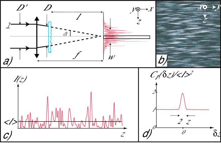
Figure 1: a) Experimental realization of the speckle pattern. A laser beam of diameter $D^{\prime}$ and wavelength $\lambda$ is first focussed by a convex lens. The converging beam of width $D$ is then scattered by a ground glass diffuser. The transverse speckle pattern is observed at the focal plane of the lens. The scattered beam diverges to an rms radius $w$ at the focal plane. b) Image of an anisotropic speckle pattern created using cylindrical optics to induce a 1D random potential for the BEC along $Oz$. c) Zoom of the speckle pattern (the boxed region of a). d) The intensity autocorrelation function $C_{I}(\delta z)$ (defined in the text). Its width gives the typical speckle grain size $\Delta z$.

2.2 Speckle Amplitude

In a fully-developed speckle pattern, the sum of the scattered partial waves results in random real and imaginary components of the electric field whose distributions are independent and Gaussian. Consequently the speckle intensity $I$ follows an exponential law:

$$P(I)=\frac{1}{\left\langle I\right\rangle}e^{-\frac{I}{\left\langle I\right\rangle}}.$$ (2)

The amplitude of the speckle intensity modulation is defined by its standard deviation $\sigma_{I}=\sqrt{\left\langle I^{2}\right\rangle-\left\langle I\right\rangle^{2}}$. From the intensity distribution (2) it is easy to show that $\sigma_{I}=\left\langle I\right\rangle$. The probability of a speckle peak having an intensity equal to or greater than five times the average intensity is less than 1%. This will provide a reasonable estimate of the highest speckle peaks (see Figure 1c).

The average speckle intensity $\langle I\rangle$ is directly related to the intensity of the incident laser beam and to the diffusion angle of light scattered by the diffuser. This angle increases as the minimum size of the scatterers on the diffuser decreases, causing the divergence of the scattered beam to increase, thereby reducing the average intensity. Reducing the distance $l$ of the diffuser from the focal plane (see Figure 1a) changes the average intensity of the speckle as the laser beam diverges over a shorter distance, but without changing the second-order statistical properties, as we will see in the following.

2.3 Speckle grain size and intensity correlation function

Roughly speaking a speckle pattern is a spatial distribution of grains of light intensity with random magnitudes, sizes and positions (see Figure 1b). The speckle grain size is characterized by the width of the intensity autocorrelation function (Figure 1d):

$$C_{I}(\delta\mathbf{r})=\left\langle I(\mathbf{r})I(\mathbf{r}+\delta\mathbf{r})\right\rangle$$ (3)

where $I(\mathbf{r})$ is the intensity at point $\mathbf{r}$ and the brackets imply statistical averaging. This function can be derived from the electric field statistics at the diffuser by Fresnel/Kirchoff theory of diffraction [29, 30]. In the focal plane of the lens, assuming paraxial approximation, the speckle electric field amplitude is the Fourier transform of the electric field transmitted by the diffuser. Thus the transverse autocorrelation function depends only on the linear phase terms of the electric field. However, in the longitudinal direction, the quadratic terms of the phase must be taken into account, leading to a different scaling in the longitudinal direction [29].

For the simple case where the diffuser is illuminated by a uniform rectangular light beam of width $D_{Y}$ and length $D_{Z}$ (as in our experiment), the intensity correlation functions in the transverse and longitudinal directions are respectively [29]:

$$C_{I}^{\bot}(\delta y,\delta z)\; = \;\left<I\right>^{2}\left[1+f\left(\frac{D_{Y}}{\lambda l}\delta y\right)f\left(\frac{D_{Z}}{\lambda l}\delta z\right)\right],$$ (4)

$$C_{I}^{\|}(\delta x)\; = \;\left<I\right>^{2}\left[1+g\left(\frac{D_{Y}^{2}}{\lambda l^{2}}\delta x\right)g\left(\frac{D_{Z}^{2}}{\lambda l^{2}}\delta x\right)\right].$$ (5)

Here $f(u)=[\sin(\pi u)/\pi u]^{2}$ is the Fourier transform of the aperture, $g(u)=\frac{2}{u}\left[C^{2}\left(\sqrt{\frac{u}{2}}\right)+S^{2}\left(\sqrt{\frac{u}{2}}\right)\right]$ where $C(s)$ and $S(s)$ are the Fresnel cosine and sine integrals respectively. Equation (4) is valid in the far-field regime, i.e. for $(\delta x^{2}+\delta y^{2})/l^{2}<<1$. We define the typical size of the speckle grains as the distance to the first zero of the functions $\frac{C_{I}(\delta\mathbb{r})}{C_{I}(0)}-1$ in each coordinate direction. We find the following grain sizes for each of the three directions:

$$\Delta y=\lambda\frac{l}{D_{Y}}\ ,\ \Delta z=\lambda\frac{l}{D_{Z}}\ ,\ \Delta x\simeq 7.6\lambda\frac{l^{2}}{D_{Y}D_{Z}}=\frac{7.6\Delta y\Delta z}{\lambda}.$$ (6)

An important point here is that aberrations of the optical setup have no effect on the properties of the speckle observed in the image plane [29]. It is interesting to note the transverse speckle grain size corresponds to the diffraction limit, i.e. it is controlled by the half-angle $\alpha=D^{\prime}/2f$ subtended by the illuminated area of the diffuser at the observation point (see Figure 1a). As a consequence, changing the distance of the diffuser relative to the lens does not change the speckle grain size along $Oz$ since the angle $\alpha$ remains constant. We also point out that the speckle grain size in the focal plane of the lens is independent of the size of the scatterers on the diffuser. We note that the longitudinal grain size $\Delta x$ is related to the transverse area $\Delta y\Delta z$ as the Rayleigh length of a gaussian beam is related to the beam waist area (within a numerical factor). Finally, we point out that when the half-angles in the transverse planes $xOz$ and $xOy$ which determine the value $\Delta z$, $\Delta y$ respectively are different, as in the experiment [see Figure 1b], an anisotropic speckle pattern is created. As we will explain in Section 3, using an anisotropic speckle pattern allows us to work with a 1D random potential for the atoms.

2.4 Self-averaging properties of a speckle pattern

A 1D random potential $v(z)$, such as a speckle pattern, can be defined by its statistical moments, ensemble averaged over the disorder. Within this statistical definition, one can generate many different realizations of the random potential. Experimentally, this can be achieved by using different ground glass diffusers or by shining different (uncorrelated) regions of the speckle pattern onto the atom cloud. In principle, experimental observations of cold atoms in a random potential will depend on the microscopic details of each particular realization of the random potential. Therefore, macroscopic transport properties, which depend only on the statistics of the random potential, should be extracted by ensemble averaging over many different realizations.

It is well known however that a spatially homogeneous (i.e. infinite) disorder, without infinite range correlations, ensures that all extensive physical quantities are “self-averaged” [32]. If a random potential is self-averaging, we can obtain the statistical moments $m_{i}$ by integrating a single realization of the random potential over an infinite range: $m_{i}=\mathrm{lim}_{[D\rightarrow\infty]}\frac{1}{D}\int_{D}\ dz\ v^{i}(z)$ for $i=1...\infty$. There is then no need to average over many different realizations as each gives exactly the same result. The fact that the spatial average coincides with the statistical average is equivalent to the well-known ergodic hypothesis in statistical mechanics, which assumes that temporal mean is equal to the statistical average. In experiments, studies are obviously carried out in finite systems, in which the self-averaging property is no longer strictly valid. However, if the length $d$ of a 1D system is sufficiently large (typically $d>>\Delta z$), the system will be approximately self-averaging. More precisely, this approximation will be valid if the statistical moments, evaluated over a finite length $d$: $m_{i}(d)~{}=~{}\frac{1}{d}\int_{-d/2}^{d/2}dz\ v^{i}(z)$, yield values sufficiently close to the ensemble averaged $m_{i}$.

In practice, it is useful to quantify the precision of this approximation. This will identify under which circumstances it is necessary to average experimental results over several realizations of disorder, and under which circumstances it is possible to assume self-averaging. For infinite systems ($d=\infty$), the self-averaging property implies $\sigma^{2}_{m_{i}}(\infty)=<m_{i}(\infty)^{2}>-<m_{i}(\infty)>^{2}=0$, so the calculation of the standard deviation $\sigma_{m_{i}}(d)$ of the moment $m_{i}(d)$ gives a non-zero value which can be used to test the extent to which a finite system is self-averaging. Rather than calculating all the standard deviations, we will focus on just the first and second-order deviations $\sigma_{m_{1}}(d)$ and $\sigma_{m_{2}}(d)$. We will see later that the second-order moment is a key parameter in our understanding of the transport properties of the BEC.

We consider a 1D speckle potential $I(z)=\sigma_{I}v(z)$ with a finite spatial correlation length $\Delta z$, where $v(z)$ is a normalized speckle field: $<v(z)>=1$ and $<v^{2}(z)>=2$. For simplicity let us approximate the auto-correlation function of the speckle pattern to unity plus a Gaussian [this happens to be a good approximation when the true auto-correlation function is $C_{v}(z)=1+\frac{\sin[\pi z/\Delta z]}{\pi z/\Delta z}$; see Figure 2]. It is then possible to obtain a simple analytical formula for $\sigma_{m_{2}}(d)$ [see A and Equation (32)-(33)]. In the asymptotic limit $d\gg\Delta z$, $\sigma_{m_{2}}(d)$ reduces to [see Equation (34)-(35)]:

$$\sigma_{m_{2}}(d)/\sigma_{m_{2}}(0)\ \simeq\ 0.959\ \sqrt{\frac{\Delta z}{d}},$$ (7)

where $\sigma^{2}_{m_{2}}(0)=<v(z)^{4}>-<v(z)^{2}>^{2}=20$. As expected, when the length $d$ of the medium tends to infinity, the system becomes self-averaging and $\sigma_{m_{2}}(d)$ tends to zero. The asymptotical convergence towards a self-averaging disorder is however slow and scales as $\sqrt{\Delta z/d}$ where $d/\Delta z$ is the typical number of peaks present within the length $d$ of the system. This scaling can be interpreted using discrete variables. If we consider the amplitude $v(z_{\rm{k}})$ of the random potential at the points $z_{\rm{k}}=\rm{k}\Delta z$, we obtain a set of independent variables $\left(v(z_{\rm{k}})\right)_{\rm{k}=1..N}$ with the statistics of the speckle intensity. Then the normalized spatial average $m_{2}(d)$ is a normalized mean value over ${\rm N}=d/\Delta z$ independent variables, which scales like $1/\sqrt{{\rm N}}$.

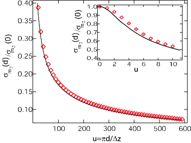
Figure 2: Normalized standard deviation $\sigma_{m_{2}}(d)/\sigma_{m_{2}}(0)$ as a function of the length $d$ of the system. Lozenges $\lozenge$ correspond to the numerical calculation of $m_{2}(d)$ with the true auto-correlation function $C_{v}(z)=1+\frac{\sin[\pi z/\Delta z]}{\pi z/\Delta z}$. The solid black line represents the analytical solution of Equation (32)-(33). Inset: shows plot in detail for small values of $d$.

In Figure 2 we plot $\sigma_{m_{2}}(d)$ for the numerical calculation using the true auto-correlation function $C_{v}(z)=1+\frac{\sin[\pi z/\Delta z]}{\pi z/\Delta z}$ (lozenges $\lozenge$) and the analytical solution with the Gaussian auto-correlation function (solid black line). Both give similar values for $\sigma_{m_{2}}(d)$. The asymptotic approximation Equation (7) is very good even for relatively small values of $d/\Delta z$: the deviation of Equation (7) from the exact solution of $\sigma_{m_{2}}(d)$ with the Gaussian approximation is less than $1\%$ when the system is larger than six times the size of the speckle grain. We note that the deviation from a self-averaging system displayed by the first-order moment $m_{1}(d)$ is very similar to that of the second-order moment (see A). For a typical number of peaks $d/\Delta z$ larger than 100 as in our experiment, the difference between the second order moment of a finite speckle pattern and that of an infinite, self-averaging one is less than 10$\%$.

3 Experimental implementation and characterization of the speckle pattern

3.1 Shining a speckle pattern onto the atomic cloud

In our experiment the random potential is superimposed on the atoms by shining a laser beam through a ground glass diffuser as shown in Figure 3. The atoms are located in the focal plane of the lens (the observation plane in Figure 1), at a distance $l=6\,$cm from the diffuser. The laser beam is derived from a tapered amplifier, injected by a free-running diode laser at $\lambda\sim 780$ nm and fibre-coupled to the experiment. The out-coupled beam is focused onto the condensate, the fibre out-coupler and lenses being mounted on a single small optical bench, aligned perpendicular to the long axis of the cigar-shaped BEC.

The optical dipole potential $V(z)$ resulting from the speckle pattern is (see Equation (1)):

$$\langle V(z)\rangle=\sigma_{V}=\frac{2}{3}\frac{\hbar\Gamma^{2}}{8I_{\rm{sat}}}\frac{\sigma_{I}}{\delta}.$$ (8)

In these experiments as in that of [26], we use a blue-detuned light, ($\delta\gtrsim 0.15\,$nm), so the potential is repulsive and the speckle grains thus act as barriers for the atoms. This is in contrast to the case of a red-detuned light ($\delta<0$) where the speckle grains act as potential wells and where atoms could be trapped by the gaussian intensity envelope of the laser beam. For the laser intensities used in these experiments, the mean speckle potential $\sigma_{V}$ is always smaller than the chemical potential of the initially trapped condensate. We define the normalized amplitude of the random potential $\gamma=\sigma_{V}/\mu_{\rm{TF}}$ relative to the Thomas-Fermi chemical potential $\mu_{\rm{TF}}$ of the initially trapped condensate. In our experiments, $\gamma$ is always smaller than unity.

As explained in Section 2.3, we can create an anisotropic speckle pattern by controlling the shape of the laser beam incident on the diffuser. We use a set of cylindrical optics such that in the $xOy$ plane (Figure 3a) the out-coupled beam from the fibre is directly focussed onto the atoms. Thus along $Oy$ the height of the beam incident on the diffuser is small, $D_{Y}=0.95\,$mm, giving a speckle grain size $\Delta y=49\,\mu$m. In the $xOz$ plane (Figure 3b), the beam is first expanded before being focussed onto the atoms and the horizontal size of the beam on the diffuser is $D_{Z}=55\,$mm, giving a horizontal grain size $\Delta z=0.85\,\mu$m. The longitudinal grain size is $\Delta x=406\mu$m. With our cigar-shaped Bose-Einstein condensates elongated along $Oz$, of transverse radius $R_{\rm{TF}}=1.5\,\mu$m and longitudinal half-length $L_{\rm{TF}}=150\,\mu$m along $Oz$, we have:

$$L_{\rm{TF}}\gg\Delta z\ \mathrm{and}\ R_{\rm{TF}}\ll\Delta y,\Delta x,$$ (9)

and the speckle pattern can be considered as a one-dimensional potential for the condensate.

The scattered laser beam has a total power of up to 150 mW and diverges to rms radii $w_{y}$ and $w_{z}$ which are two orders of magnitude larger than $R_{\rm{TF}}$ and $L_{\rm{TF}}$ respectively at the condensate. Therefore the average intensity (the Gaussian envelope) of the beam can be assumed constant over the region where the atoms are trapped.

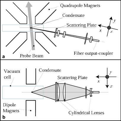
Figure 3: Optical setup used to create the speckle potential. The BEC is at the focus of the lens system with its long axis oriented along the $z$ direction. The two figures are shown in the same scale. The beam incident on the diffuser has different widths in the $y$ and $z$ directions, which leads to anisotropic speckle grains (see text). a) Side view. b) Upper view.

3.2 Calibration of the speckle grain size

In principle, the size of the speckle grains $\Delta z$ can be calculated from the parameters $l$ and $D$ of the optical system. However, a large aperture cylindrical lens system is not stigmatic and we have therefore calibrated the speckle grain size using images from a CCD camera. The optical set-up is removed from the BEC apparatus and the intensity distribution observed on a CCD camera at the same distance $l$ as the atoms. Taking images with various beam apertures $D_{Z}$, we determine the autocorrelation function of the speckle patterns to obtain the grain size $\Delta z$ that we plot versus $1/D_{Z}$. For speckle grain sizes larger than the CCD camera pixels ($2\,\mu$m), we can fit the data with a straight line, obtaining $\Delta z=1.11(9)\times\lambda l/D_{Z}$ to be compared with the calculated grain $\Delta z=\lambda l/D_{Z}$ with the paraxial assumption. The camera cannot resolve speckle grains smaller than the pixel size and so we extrapolate the fit to give the grain size corresponding to the aperture we use: for $D_{Z}=55\,$mm, we obtain $\Delta z=0.95(7)\,\mu$m. The width of the auto-correlation function in the perpendicular axis gives the experimental value $\Delta y=54(1)\,\mu$m, leading to the longitudinal size $\Delta x=499(38)\,\mu$m.

3.3 Calibration of the speckle average intensity via light shift measurements

Obtaining a reliable value for a dipolar potential from a photometric measurement of light intensity is notoriously difficult. In our case, an additional problem arises due to the strong focussing, entailing a strong variation of the intensity along the beam axis $Ox$. The ideal method to calibrate the dipolar potential is to use the atoms themselves as a sensor. This potential is nothing else than the light-shift of the lower level, $F=1$ in our case. In order to relate this light-shift to the directly measured power of the laser that creates the speckle random potential, we have used a measurement of the differential light-shift of the $F=1\rightarrow F=2$ hyperfine transition.

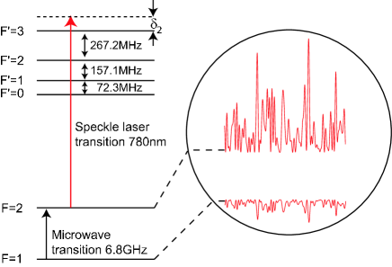
Figure 4: The speckle light at 780 nm induces a light shift in both $F=1$ and $F=2$. Tuning the speckle laser close to the $F=2$ level as shown creates a spatially varying differential light-shift on the 6.8 GHz transition.

The condensate is magnetically trapped in the $|F\!=\!1,\,m_{F}\!=\!-1\,\rangle$ sublevel (Figure 4). We use a microwave frequency generator and antenna to drive the 6.8 GHz $\sigma^{+}$ transition to the $|F\!=\!2,\,m_{F}\!=\!0\rangle$ sublevel. Atoms coupled into this state are then lost from the trap. By monitoring the number of atoms remaining in $|F\!=\!1,\,m_{F}\!=\!-1\,\rangle$ as a function of microwave frequency $f_{\rm{mw}}$, we obtain a spectrum of this transition.

When the speckle laser is shone onto the atoms, both ground-states $F=1$ and $F=2$ are light-shifted and the microwave spectrum is modified. To produce a substantial differential light shift on the transition, we must tune the speckle laser close to resonance for either the $F=1$ or $F=2$ state. We chose to tune the laser close to the $F=2\rightarrow F^{\prime}=3$ transition frequency, to minimize spontaneous scattering by the atoms trapped in the $F=1$ level. Then the speckle laser is sufficiently detuned from $F=1\rightarrow F^{\prime}$ transitions ($\delta_{1}\sim 6.8$ GHz) that the hyperfine structure of the upper $F^{\prime}$ levels is not resolved for this transition and the light-shift of the $|F\!=\!1,\,m_{F}\!=\!-1\,\rangle$ sublevel is calculated using Equation (8) [the transition strength is $2/3$ for $\pi$-polarized light]. For the $F=2\rightarrow F^{\prime}$ transitions, one has to take into account the hyperfine structure of the excited state $F^{\prime}$. The $\pi$-polarized speckle laser beam couples the $|F\!=\!2,\,m_{F}\!=\!0\,\rangle$ sublevel to $|F^{\prime}\!=\!1,\,m_{F}\!=\!0\,\rangle$ and $|F^{\prime}\!=\!3,\,m_{F}\!=\!0\,\rangle$ with the transition strengths 1/15 and 3/5 respectively. For detunings close to resonance with $F=2\rightarrow F^{\prime}=3$, the contribution to the light-shift of the transition to the $F^{\prime}=1$ sublevel is negligible at the 1% level. In this approximation we obtain the differential light-shift of the transition:

$$\Delta E = \frac{\hbar\Gamma^{2}}{8I_{\rm{sat}}}\ I\left(\frac{3}{5}\frac{1}{\delta_{2}}-\frac{2}{3}\frac{1}{\delta_{1}}\right)$$

$$\simeq \frac{3}{5}\frac{\hbar\Gamma^{2}}{8I_{\rm{sat}}}\frac{I}{\delta_{2}}\quad\rm{for}\ \delta_{2}\ll\delta_{1}$$

where $\delta_{1}$ is the detuning relative to the $F=1\rightarrow F^{\prime}=3$ transition, $\delta_{2}$ is the detuning relative to the $F=2\rightarrow F^{\prime}=3$ transition ($\delta_{1}=\delta_{2}-6.835$ GHz). Note that the laser is always red-detuned from $F=1$ by about $-6.8\,$GHz, so creates an attractive speckle potential for the atoms, while it is red or blue-detuned for the $F=2$ state. Atoms transferred to $F=2$ by the microwave pulse will be rapidly lost due to near resonant spontaneous scattering.

Spectra obtained for a condensate in the absence of the speckle potential (red crosses $+$ on Figure 5a) have a width of $\simeq 15\,$kHz and are shifted by $f_{B}=f_{\rm{mw}}-6.8$GHz $\simeq-2800\,$kHz from the $F=1\rightarrow F=2$ transition frequency. This shift and this width are due to the Zeeman effect on the magnetic $|F\!=\!1,\,m_{F}\!=\!-1\,\rangle$ sublevel: the minimum magnetic field $B_{0}$ of the Ioffe trap shifts the frequency transition by $f_{B}=g_{F}\mu_{B}B_{0}/h$ and the curvature of the magnetic trap over the region of the condensate broadens the spectrum towards lower frequencies. When the speckle laser is shone on the atoms, different atoms experience different light-shifts due to the spatial modulations of intensity in the speckle pattern. The spectrum is therefore inhomogeneously broadened due to the range of light intensities, as shown in Figure 5a. For these measurement we used speckle intensities of $\langle I\rangle\lesssim 0.3\,$mW. cm^-2 and detunings $\delta_{2}$ from -15 MHz to -500 MHz.

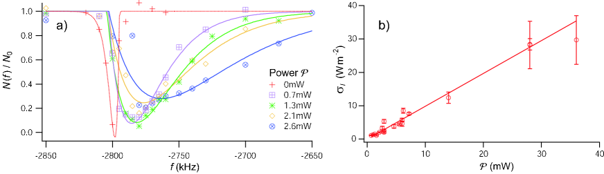
Figure 5: a) Fraction of atoms remaining in $F=1$ after a 5 ms pulse of microwaves at frequency $f_{\rm{mw}}=6.8\rm{GHz}+f$, for speckle laser powers $\mathcal{P}$ indicated and fixed (blue) detuning $\delta=15\,$MHz. Increasing the speckle laser power broadens the spectra to lower microwave frequencies. (Frequency $f$ is indicated relative to the unshifted transition frequency at 6.834683 GHz.) The solid lines represent fits to Equation (15). b) $\sigma_{I}$ versus speckle laser power $\mathcal{P}$. The fit gives $\sigma_{I}/\mathcal{P}=1.0(1)\times 10^{3}\rm{m}^{-2}$.

In order to calibrate the dipolar potential and to extract the average intensity $\sigma_{I}$ from these experimental spectra, we have developed a simple model. Since the broadening of the spectra due to the variation of the speckle intensity is very large compared with the Zeeman broadening we neglect the latter. Approximating to a constant density profile, we use the statistics of the speckle intensity distribution to model the evaporation. Since the mean potential $\sigma_{V}$ is typically 100 times greater than the chemical potential of the condensate, we assume that the atoms are located essentially at the maxima of the speckle intensity peaks (minima of the trapping potential). The number of atoms remaining after application of the microwave pulse at frequency $f_{\rm{mw}}=6.8\,$GHz$+f$ is then:

$$N(f)=N_{0}\left[1-\alpha\frac{\Delta f}{3\Gamma^{2}/80\pi I_{\rm{sat}}\delta_{2}}P^{\prime}(I(f))\right]=N_{0}\left[1-\mathcal{A}P^{\prime}(I(f))\right]$$ (11)

where $\alpha$ is the coupling efficiency of the microwave knife and $\Delta f$ the frequency width coupled by the microwave knife, $I(f)$ is the intensity resonant with the frequency $(f-f_{B})$, i.e.

$$h(f-f_{B})=\frac{3\hbar\Gamma^{2}I(f)}{40I_{\rm{sat}}\delta_{2}}.$$ (12)

In Equation (11) $P^{\prime}(I)$ is the distribution of ‘nearest local maxima’ of intensity given by:

$$P^{\prime}(I^{\prime})=\frac{4I^{\prime}\exp(-2I^{\prime}/\bar{I^{\prime}})}{\bar{I}^{{}^{\prime}2}}$$ (13)

where $\bar{I}^{{}^{\prime}}=1.89\sigma_{I}$ is the average value of the distribution of intensity maxima. Equation (13) is obtained by simulations of the speckle distribution in which the intensity $I$ at each point of the speckle random potential was replaced by the intensity at the nearest maximum $I^{\prime}$ (see Figure 6).

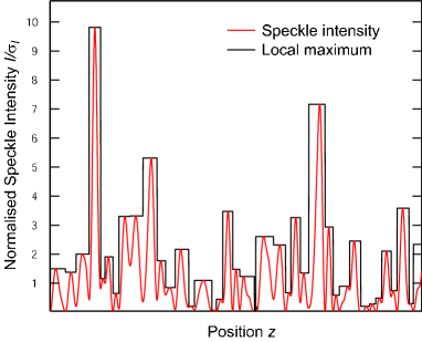
Figure 6: Plot of the ‘nearest local maxima’ effective potential (black line) of one realization of the speckle pattern (red line). We use this simulation to obtain the probability distribution of the ‘nearest local maxima’ $P^{\prime}(I)$.

We finally obtain from Equation (11)-(13):

$$N(f)=N_{0}\left[1-\mathcal{B}\frac{(f-f_{B})}{(1.89\sigma_{I})^{2}}\exp\left(-2\frac{f-f_{B}}{1.89(f_{\sigma_{I}}-f_{B})}\right)\right]$$ (14)

where $\mathcal{B}=320\pi\mathcal{A}I_{\rm{sat}}\delta_{2}/3\Gamma^{2}$.

In the experiment, we measure the power $\mathcal{P}$ at the input of the optical setup that creates the speckle random potential. The aim of the calibration is thus to relate $\mathcal{P}$ to the average intensity $\sigma_{I}$ of the random potential on the atoms. In order to extract $\sigma_{I}$ from the experimental data we fit the spectra in Figure 5a with a function similar to Equation (14):

$$N(f)=N_{0}\left[1-\mathcal{C}(f-f_{B})\exp\left(-2\frac{f-f_{B}}{1.89(f_{\sigma_{I}}-f_{B})}\right)\right]$$ (15)

where $\mathcal{C}$, $f_{B}$ and $f_{\sigma_{I}}$ are fitting parameters. Plotting the fitted values of $f_{\sigma_{I}}$ versus $\mathcal{P}/\delta_{2}$ for red- and blue-detuned light we then obtain a more accurate value of $f_{B}$ than that obtained by fitting Equation (15) to each individual spectrum. Using Equation (12) we obtain $\sigma_{I}$ from $f_{\sigma_{I}}-f_{B}$ and plot $\sigma_{I}$ versus $\mathcal{P}$ in Figure 5b. We obtain $\sigma_{I}/\mathcal{P}=1.0(1)\times 10^{3}\rm{m}^{-2}$ as the calibration constant relating the power $\mathcal{P}$ to the average speckle intensity at the atoms $\sigma_{I}$.

4 Expansion in a 1D waveguide : a study of transport properties of a Bose-Einstein condensate in a speckle random potential

4.1 Production of a condensate of ⁸⁷Rb atoms

We produce a Bose-Einstein condensate of ⁸⁷Rb atoms in the $|F=1,m_{F}=-1>$ hyperfine state. The design of our iron-core electromagnet allows us to create an elongated Ioffe-Pritchard magnetic trap with axial and radial frequencies of $\omega_{z}=2\pi\times 6.70(7)$ Hz and $\omega_{\perp}=2\pi\times 660(4)$ Hz respectively. The magnetic trap is loaded from a magneto-optical trap (MOT) and the atom cloud is cooled down to quantum degeneracy (BEC) using a radio-frequency (rf) evaporation ramp. Typically, our BECs comprise 3.5 $\times 10^{5}$ atoms and are characterized by a chemical potential $\mu_{\rm{TF}}/2\pi\hbar\sim 4.6$ kHz and Thomas-Fermi half length $L_{\rm{TF}}=150$ $\mu$m and radius $R_{\rm{TF}}=1.5$ $\mu$m. Further details of our experimental apparatus are presented in [33].

The large aspect ratio of the trap is of primary importance for the experiments described in this article. As stated in Section 3.1 the large anisotropy of the speckle grains ($\Delta x=499(38)\,\mu$m, $\Delta y=54(1)\,\mu$m and $\Delta z=0.95(7)\,\mu$m) help us to obtain a 1D random potential for the atoms. Yet to work with true 1D random potentials, i.e. $L_{\rm{TF}}/\Delta z\gg 1$ and $R_{\rm{TF}}/\Delta x\ll 1$, an order of magnitude difference between the sizes $L_{\rm{TF}}$ and $R_{\rm{TF}}$ of the BEC is needed. With the aspect ratio of our magnetic trap we have $L_{\rm{TF}}/\Delta z\simeq 158$ and $R_{\rm{TF}}/\Delta x\simeq 0.03$.

4.2 Axial expansion: opening the longitudinal trap

To study the coherent transport of the BEC in the random potential, we observe the longitudinal expansion of the condensate in a long magnetic guide. The setup of our magnetic trap allows us to control almost independently the longitudinal and transverse trap frequencies by changing the currents in the axial and radial excitation coils. By reducing the axial confinement without modifying the transverse confinement, we create a 1D magnetic waveguide for the condensate. Repulsive inter-atomic interactions drive the longitudinal expansion of the BEC along this guide.

Reducing the current in the axial excitation coils reduces both the longitudinal trap frequency and the minimum value of the magnetic field. If the minimum magnetic field crosses zero, atoms can undergo Majorana spin-flips from the trapped hyperfine state $|F=1,m_{F}=-1>$ to non-trapped hyperfine states and are then lost from the trap. Therefore we monitor the atom number as a function of the axial current in order to determine the current at which the magnetic field crosses zero. This zero-crossing defines a lower limit for the axial current and so we reduce the axial trap frequency $\omega_{z}/2\pi$ to a final value slightly above this limit. Since we cannot reduce the axial field curvature strictly to zero, a small longitudinal trapping remains. By observing dipole and quadrupole oscillations (at frequencies $\omega^{\prime}_{z}$ and $\sqrt{2/5}\ \omega^{\prime}_{z}$ respectively) in the magnetic waveguide, we measured $\omega^{\prime}_{z}/2\pi=1.10(5)$ Hz for the residual trapping frequency in the guide.

Opening the trap abruptly induces atom loss and heating of the atom cloud, therefore the trap is ramped over 30 ms to avoid these processes. Once the current in the axial coils has reached its final value we have a BEC of N $\sim 2.5\times 10^{5}$ – $3\times 10^{5}$ atoms in the magnetic guide.

To perform the experiment in the presence of the random potential, we use the following procedure. After creating the condensate of ⁸⁷Rb atoms we shine the random potential onto the atoms and wait 200 ms for the BEC to reach equilibrium in the combined initial trap and disorder potential. We then open the longitudinal confinement, switch off the evaporation RF knife and the BEC expands in the 1D waveguide in the presence of disorder due to repulsive interactions. We turn off all remaining fields (including the random potential) after a total axial expansion time $\tau$ (which includes the 30 ms opening time of the axial trap) and wait a further $t_{\rm{tof}}=15$ ms of free fall before imaging the atoms by absorption.

4.3 Image analysis and longitudinal density profiles

In our experiment we obtain quantitative information about the atom cloud by taking absorption images after a time-of-flight $t_{\rm{tof}}$=15 ms. Absorption imaging effectively integrates the atomic density along the direction of the imaging beam $Oy$, such that we measure the 2D density after time-of-flight $n_{\rm{2D}}(x,z,t_{\rm{tof}})$.

In the harmonic trap ($\tau=0$) without disorder, the Thomas-Fermi condition is fulfilled and this justifies the use of the scaling theory [34]. During the time-of-fligth $t_{\rm{tof}}$, the atom cloud expands with the scaling factors $\lambda_{\perp}(t_{\rm{tof}})$ and $\lambda_{z}(t_{\rm{tof}})$ in the radial and longitudinal directions respectively. In our elongated trap $\lambda_{z}(t_{\rm{tof}})\simeq 1$ and, after a time-of-flight $t_{\rm{tof}}$, we have:

$$n_{\rm{2D}}(x,z,t=t_{\rm{tof}})=\frac{1}{\lambda_{\perp}(t_{\rm{tof}})}\ n_{\rm{2D}}\left[\frac{x}{\lambda_{\perp}(t_{\rm{tof}})},z,t=0\right].$$ (16)

In the magnetic waveguide, the radial frequency $\omega_{\perp}$ is unchanged. When the longitudinal expansion is stopped, i.e. when there is no longitudinal kinetic energy, the energy of atom cloud is also totally transferred to the transverse degree of freedom during $t_{\rm{tof}}$ with the scaling factor $\lambda_{\perp}$ of the initial trap. Then Equation (16) is still valid to describe the expansion of the condensate from the magnetic waveguide during the time-of-flight. Therefore the 2D density before time-of-flight is $n_{\rm{2D}}(x,z,\tau)=\lambda_{\perp}(t_{\rm{tof}})\ n_{\rm{2D}}(\lambda_{\perp}(t_{\rm{tof}})x,z,\tau+t_{\rm{tof}})$ where $\tau$ is the time spent by the BEC in the waveguide. In the waveguide in presence of a random potential, the 3D density can be written as:

$$n_{\rm{3D}}(x,y,z,\tau)=\frac{1}{g}\left[\mu(\tau)-m\omega_{\perp}^{2}x^{2}/2-m\omega_{\perp}^{2}y^{2}/2-V(z)\right],$$ (17)

where $\mu(\tau)$ is the chemical potential in presence of the 1D random potential $V(z)$, $g=\frac{4\pi\hbar^{2}a}{m}$ is the interaction parameter and $a$ is the scattering length. Then the 2D density is:

$$n_{\rm{2D}}(x,z,\tau)=\int\ dy\ n_{\rm{3D}}(x,y,z,\tau)=\frac{4R_{\rm{TF}}}{3g\sqrt{\mu_{\rm{TF}}}}\left[\mu(\tau)-m\omega_{\perp}^{2}x^{2}/2-V(z)\right]^{3/2}.$$ (18)

In particular, assuming the amplitude of the random potential $<V>=\sigma_{V}$ is small compared to the chemical potential $\mu$, $\sigma_{V}\ll\mu$, we have $n_{\rm{2D}}(x=0,z,\tau)\simeq\frac{4R_{\rm{TF}}\mu(\tau)^{3/2}}{3g\sqrt{\mu_{\rm{TF}}}}$ up to first order in $\sigma_{V}/\mu$.

From these 2D images, we extract the “longitudinal density profile” $n_{\rm{2D}}(x=0,z,\tau)$ and use it to calculate the rms length $L$ and the centre-of-mass position of the expanding condensate in the absence or presence of the random potential.

4.4 Expansion of the BEC and time evolution of rms length $L$

We measure the rms size $L$ and the centre-of-mass position of the condensate as a function of the longitudinal expansion time $\tau$ and plot these quantities as a function of $\omega_{z}\tau$ in Figure 7. The expansion of the condensate in the 1D waveguide without disorder ($\gamma$=0) is linear as predicted by the scaling theory [34]. When the 1D random potential is added ($\gamma$=0.15, 0.23, 0.28) the expansion is reduced and eventually stops as reported in [26]. The dashed lines in Figure 7a indicate $L^{\rm{f}}$, the final rms size of the condensate once it stops expanding. The data in Figure 7a indicate that the larger the normalized amplitude of the random potential compared to the initial chemical potential ($\gamma$), the shorter the final rms length $L^{\rm{f}}$ of the condensate.

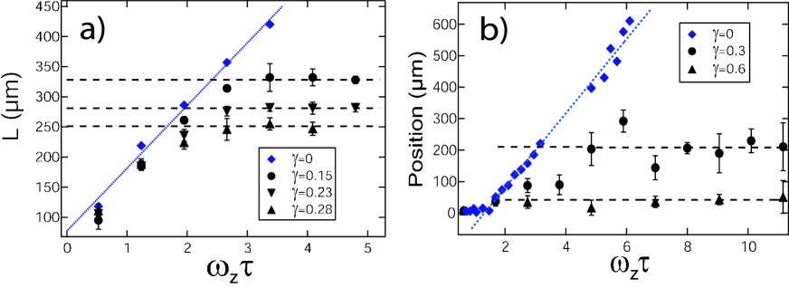
Figure 7: a) Time evolution of the rms size L of the expanding Bose-Einstein condensate in the 1D magnetic guide in presence of a 1D random potential with amplitude $\gamma=\sigma_{V}/\mu_{\rm{TF}}$. Error bars represents standard deviation over 5 realizations of the speckle pattern (dashed lines are guides to the eye) ; b) Time evolution of the centre of mass position for the different values of $\gamma$.

Figure 7b shows the centre-of-mass position of the BEC as a function of axial expansion time $\tau$. In the absence of the random potential, the condensate acquires a centre-of-mass velocity of 2.8(1) mm s^-1, due to a magnetic ‘kick’ during the longitudinal opening of the trap. We observe that applying a small amplitude random potential also inhibits this centre-of-mass motion. The displacement of the condensate decreases with increasing amplitude $\gamma$ as shown in Figure 7b. Each point in Figure 7 is obtained by averaging the experimental results over 5 different realizations of the speckle pattern. The error bars represent the corresponding standard deviations. We find that these standard deviations are not larger than the shot-to-shot deviation observed using a single realization of the random potential. We therefore claim that this system is self-averaging within our experimental resolution. Further justification is presented in Section 5.2. This self-averaging property of our system allows us to measure transport properties without averaging over many realizations of the disorder, which is an important practical advantage.

The suppression of transport of the expanding matter-wave also appears clearly on the longitudinal density profiles obtained in the experiments. We plot in Figure 8 the time evolution of the longitudinal density profiles for different values of the amplitude $\gamma$ of the random potential. The dotted red profile on every graph represents the longitudinal profile before expansion ($\tau=0$) in the absence of the random potential. This is the usual inverted parabola for a harmonically trapped Bose-Einstein condensate in the Thomas-Fermi regime. During the expansion without disorder (see Figure 8a), the shape remains an inverted parabola with the rms size increasing as expected from the scaling theory [34]. When the random potential is added (see Figure 8b and c), the longitudinal density profile changes with time. Eventually it reaches a stationary shape (corresponding to the stationary rms size on Figure 7a) with two main characteristics: (i) a constant central density (with random spatial modulations) and (ii) steep edges demarcating this central region.

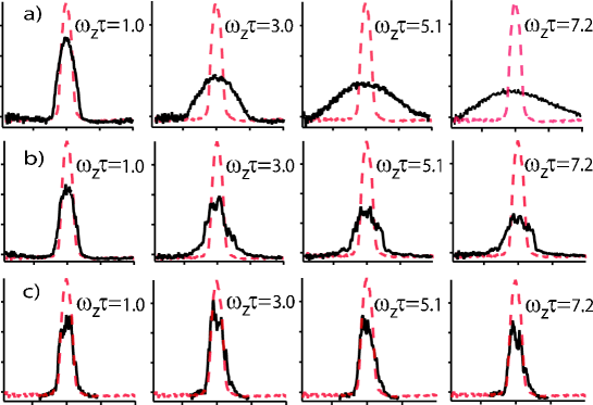
Figure 8: Longitudinal density profiles of the expanding BEC for times $\omega_{z}\tau=$1.0, 3.0, 5.1 and 7.2 with a) $\gamma$=0, b) $\gamma$=0.15 and c) $\gamma$=0.3. The dotted (red) line is the longitudinal profile in the initial trap ($\tau=0$) in the absence of disorder.

Our experimental results clearly show the suppression of transport of a coherent matter-wave induced by a random potential [26]. Although phenomenologically similar to a single particle Anderson localization (AL), we have argued in Refs.[12, 26] that, in the mean-field regime of our experiment where interactions are weak but interaction energy dominates over the kinetic energy, the physics strongly changes compared with that of AL with non-interacting bosons. In the following we investigate experimentally the scenario of disorder-induced trapping of an interacting Bose-Einstein condensate in the mean field regime proposed in Refs.[12, 26].

5 Experimental characterization of the disorder-induced trapping scenario

5.1 The disorder-induced trapping scenario of an elongated BEC

The disorder-induced trapping scenario proposed in [12, 26] describes the expansion of a 1D interacting matter-wave in a 1D random potential in a regime where interactions dominate over the kinetic energy. The dynamics of the BEC is governed by three kinds of energy: the amplitude of the random potential, the kinetic energy of the atoms and the inter-atomic interaction energy. The relative importance of each of these three energy contributions depends on the local density of the BEC. At the centre of the condensate where the density remains large, interactions play a crucial role and the kinetic energy is negligible. In contrast, the wings are populated by fast atoms with a low density and therefore the kinetic energy dominates over the interaction energy. Let us briefly describe what happens in each of these regions.

In the wings, the kinetic energy dominates over the interaction energy. The fast, weakly interacting atoms which populate the wings undergo multiple reflections and transmissions on the modulations of the random potential (see numerical simulations in [12, 26]). Trapping finally results from a classical reflection on a large modulation of the random potential. The density in the wings of the disorder-trapped BEC is too small to be measured by absorption imaging in our experiment.

We will now focus on the behaviour in the centre of the BEC. Following the definitions of [12], we arbitrarily delimit the core of the BEC as half the size of the initial condensate: $-L_{\rm{TF}}/2<z<L_{\rm{TF}}/2$. During the expansion of the condensate in the waveguide, the density at the centre of the cloud slowly decreases. It is thus possible to define a quasi-static effective chemical potential $\mu_{\rm{eff}}(\tau)$ for the core of the BEC after an expansion time $\tau$ in the magnetic guide. The kinetic energy is small, the time evolution is quasi-static and the healing length $\xi=0.11~{}\mu$m remains much smaller than the correlation length of the speckle potential $\Delta z=0.95~{}\mu$m: thus the Thomas-Fermi approximation is valid. As a consequence, the random potential modulates the density and the calculation of $\mu_{\rm{eff}}(\tau)$ requires averaging over the length of the core. The effective chemical potential $\mu_{\rm{eff}}(\tau)$ is simply the sum of the interaction energy and the random potential energy and is defined as $\mu_{\rm{eff}}(\tau)=\frac{1}{L_{\rm{TF}}}\int_{-L_{\rm{TF}}/2}^{L_{\rm{TF}}/2}dz\ [g\ n_{\rm{3D}}(x=0,y=0,z,\tau)\ +\ V(z)]$. The rapid lost of the overall parabolic shape during the initial expansion of the BEC in the random potential (see Figure 8 and [12]) justifies this expression for $\mu_{\rm{eff}}(\tau)$ with no longitudinal magnetic trapping term. The effective chemical potential $\mu_{\rm{eff}}(\tau)$ slowly decreases with the density during the axial expansion time $\tau$ and eventually drops to a value smaller than the amplitude of some peaks of the speckle potential. Once this situation is reached, the condensate is trapped in the region between these peaks and it fragments [12, 26]. The criterion for trapping the core of the BEC is the existence of two large modulations of the random potential equal or greater than the effective chemical potential $\mu_{\rm{eff}}$. Below, we adapt the calculations of [12] for 1D BECs to take into account the transverse extension of our 3D atom cloud. We note that the calculations of [12] assume a random potential with $<V>=0$ so that the effective chemical potential reduces to the interaction term: $\mu(\tau)=\mu_{\rm{eff}}(\tau)-<V>$ . However, none of the physics of our experiment is lost by making this adjustment with the time-independent energy $<V>$. In the following we will use this new effective chemical potential $\mu(\tau)$.

As the speckle potential is truly a 1D potential we can write the condition of fragmentation in our 3D experimental BEC in the same way as it is done in [12] for a 1D BEC: the picture developed for 1D BECs holds for the experimental 3D condensates with the effective chemical potential $\mu(\tau)$ defined here. On the one hand if the BEC is fragmented at the centre ($r^{2}=x^{2}+y^{2}=0$) then the condition for fragmentation holds along the $x$-axis and $y$-axis since the density decreases as $|r|$ increases. On the other hand when the condition of fragmentation is not fulfilled at the centre of the BEC ($r=0$) the BEC expands and there is no disorder-induced trapping.

The number of peaks in the core of the BEC with energy greater than the effective chemical potential $\mu(\tau)$ is given by:

$$N_{\rm{peaks}}(V\geq\mu(\tau))\simeq 0.94\left(\frac{L_{\rm{TF}}}{\Delta z}\right)\exp\left[-0.75\frac{V}{\sigma_{V}}\right]$$ (19)

The condition of fragmentation is $N_{\rm{peaks}}=2$, and leads to a relation between the final effective chemical potential $\mu^{\rm{f}}$ once the core of the BEC is trapped and the characteristic parameters $\sigma_{V}$ and $\Delta z$ of the speckle potential. For small values of $\gamma=\sigma_{V}/\mu_{\rm{TF}}$ we obtain :

$$\mu^{\rm{f}}\simeq\frac{\mu_{\rm{TF}}}{0.75}\ \gamma\ \mathrm{ln}\left(\frac{0.47L_{\rm{TF}}}{\Delta z}\right),$$ (20)

the logarithmic term reflecting the exponential probability distribution of intensity of the speckle pattern (see Section 2.2) and $\Delta z$ the second-order statistics of our speckle potential.

Since the effective chemical potential $\mu(\tau)$ of the core of the BEC decreases during the expansion, it cannot be larger than the initial value $\mu(\tau=0)=\mu^{\rm{i}}=\frac{g}{L_{\rm{TF}}}\int_{-L_{\rm{TF/2}}}^{L_{\rm{TF/2}}}\ dz\ n_{\rm{3D}}(0,0,z)$. Integration over the core gives:

$$\mu^{\rm{i}}=\frac{11\mu_{\rm{TF}}}{12}\simeq 0.92\mu_{\rm{TF}}$$ (21)

which thus provides an upper value for $\mu^{\rm{f}}$.

In order to compare the experiments with this scenario we have to extract the effective chemical potential $\mu(\tau)$ in the core of the condensate from the data (as detailed in Section 4.3). We extract the mean density from our longitudinal profiles by averaging the density over the core of the condensate $\overline{n}_{\rm{2D}}(\tau)=\frac{1}{L_{\rm{TF}}}\int_{-L_{\rm{TF}}/2}^{L_{\rm{TF}}/2}dz\ n_{\rm{2D}}(x=0,z,\tau)$. Then the experimental effective chemical potential is [see Equation (18))]:

$$\mu(\tau)=\mu_{\rm{TF}}^{1/3}\left(\frac{3g\overline{n}_{\rm{2D}}(\tau)}{4R_{\rm{TF}}}\right)^{2/3},$$ (22)

so that $\mu(\tau)$ can be directly extracted from the measured density $n_{\rm{2D}}$.

5.2 Measurement of the average density in the core of the elongated condensate

When disorder-induced trapping occurs at the centre, the average density in the core has dropped to a final value $\overline{n}_{\rm{2D}}^{\ f}\sim\gamma\mu_{\rm{TF}}/g$ [see Equation (20)-(22)] and is then expected to remain stationary. However, because of atom losses due to processes such as evaporation, collisions, etc, the density in the core will continue to fall. In Figure 9a we plot the time evolution of the ratio of the average density $\overline{n}_{\rm{2D}}(\tau)$ over the initial one $\overline{n}_{\rm{2D}}^{\ i}$ for different amplitudes $\gamma$ of the random potential. Without the random potential (black dots $\bullet$), the time evolution of the average density is in very good agreement with the predicted expansion in the magnetic waveguide according to scaling theory (dashed black line). In the presence of the random potential, the rate of decrease of the average density $\overline{n}_{\rm{2D}}(\tau)$ is much reduced (see Figure 9a). In particular, once the core of the condensate stops expanding, the evolution of $\overline{n}_{\rm{2D}}(\tau)$ changes to an exponential decay (the solid lines in Figure 9a). This exponential decay is due to atom losses and indicates that the density is no longer decreasing due to expansion. Hence the onset of disorder-induced trapping is marked by a change of slope in the time evolution of the density $\overline{n}_{\rm{2D}}(\tau)$, and is indicated by the start of each solid line in Figure 9a). For a speckle amplitude $\gamma=0.30$, trapping occurs at $\omega_{z}\tau=0.5$. The subsequent decrease in the density $\overline{n}_{\rm{2D}}(\tau)$ ($\omega_{z}\tau>0.5$) is fitted with an exponential $\exp[-\Gamma\tau]$, giving the time constant $1/\Gamma\simeq$ 280 ms for atom losses. We then use an exponential with the same time constant $1/\Gamma$ to fit the curves corresponding to $\gamma=0.05$ and $\gamma=0.10$. The onset of this exponential decay gives us a measurement of the final average density $\overline{n}_{\rm{2D}}^{f}$ for which disorder-induced trapping occurs. In Figure 9, the error bars on $\overline{n}_{\rm{2D}}^{f}$ represent the difference in the density between the last point considered as part of the expansion and the first point marking the onset of disorder-induced trapping.

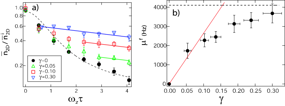
Figure 9: a) Ratio $\overline{n}_{\rm{2D}}(\tau)/\overline{n}_{\rm{2D}}^{\ i}$ of the average density to the initial density at the centre of the condensate after an expansion time $\omega_{z}\tau$ in the 1D magnetic guide for different amplitudes of the random potential $\gamma$=0, 0.05, 0.10 and 0.30. The dashed line shows the predicted time evolution according to scaling theory for $\gamma=0$. After the onset of disorder-induced trapping, atom losses lead to a purely exponential decay indicated by the solid line fits. The onset of a purely exponential decay (marked by the start of each solid line) indicates the final density $\overline{n}_{\rm{2D}}^{f}$ at which disorder-induced trapping occurs. b) Final effective potential $\mu^{\rm{f}}=\mu_{\rm{TF}}^{1/3}\left(\frac{3g\overline{n}_{\rm{2D}}^{\ f}}{4R_{\rm{TF}}}\right)^{2/3}$ at the centre of the trapped condensate as a function of the amplitude of the random potential $\gamma$. The (red) solid line corresponds to the expected slope from Equation (20). The black dashed line corresponds to the saturation value $0.92\mu$ [Equation (21)].

From the analysis of our experimental data in Figure 9a we extract the final effective chemical potential $\mu^{\rm{f}}=\mu_{\rm{TF}}^{1/3}\left(\frac{3g\overline{n}_{\rm{2D}}^{\ f}}{4R_{\rm{TF}}}\right)^{2/3}$ and plot $\mu^{\rm{f}}$ versus the speckle amplitude $\gamma$ in Figure 9b. Comparing the final effective chemical potential $\mu^{\rm{f}}$ once the core of the BEC is trapped with the amplitude $\gamma$ of the random potential allows a test of Equation (20)-(21). Indeed, according to Equation (20), the slope of the function $\mu^{\rm{f}}(\gamma)$ for small values of $\gamma$ reflects the first and second-order statistical properties of the disorder, in particular the exponential one-point distribution of intensity of the speckle and the correlation length $\Delta z$. For the parameters of our speckle potential we expect to obtain for the asymptotic value of the effective chemical potential $\mu^{\rm{f}}\simeq 26.4(2)~{}10^{3}\times\gamma$ [see Equation (20)]. The evolution of $\mu^{\rm{f}}$ at small values of $\gamma$ is in good agreement with this predicted value for the slope (red solid line on Figure 9b). For larger amplitudes $\gamma$ of the random potential, $\mu^{\rm{f}}$ saturates at a nearly constant value in agreement with Equation (21) (black dashed line in Figure 9b is the expected saturation value). We note that this clearly distinguishes between our case and the case of a lattice. In the mean-field regime with the healing length smaller than the lattice spacing, the expansion of the condensate in a lattice is never suppressed as no large peak can provide a sharp stopping [12]. However, the decrease of the average density of the BEC is stopped when the effective chemical potential $\mu$ equals the depth of the lattice $V$ (fragmentation). The dependence of the final effective chemical potential $\mu^{\rm{f}}$ with $\gamma=V/\mu_{\mathrm{TF}}$ in the case of a lattice is then $\mu^{\rm{f}}=\mu_{\rm{TF}}\times\gamma\simeq 4.6~{}10^{3}\times\gamma$, independently of the lattice spacing.

The self-averaging property of our system appears in this measurement once again. Experimentally we measure $\overline{n}_{\rm{2D}}^{\ f}$ which depends on $\sigma_{V}$ [see Equation (20)-(22)]. The average speckle amplitude $\sigma_{V}$ is related to the second order moment $m_{2}$ of the random potential. In Section 2.4 we showed that the standard deviation of moment $m_{2}$ is expected to vary as Equation (7). For our optical apparatus [$\Delta z=0.95(7)$ $\mu$m], the deviation $\sigma_{m_{2}}(L_{\rm{TF}})$ is less than 8% from one realization of the speckle potential to another . This variation is less than the experimental shot-to-shot variations of $\simeq 15\%$ on $\overline{n}_{\rm{2D}}^{\ f}$ obtained with one realization of the speckle potential. The arguments of Section 2.4 are therefore in agreement with our observations and we conclude that our system can be considered as self-averaging given our experimental resolution.

6 Conclusion

In conclusion, we have observed the suppression of transport of a coherent matter-wave of interacting particles in a 1D optical random potential. Using laser speckle patterns to create the random potential is particularly interesting as all statistical properties can be controlled accurately. We have developed a technique to calibrate the average amplitude $\sigma_{V}$ of our random potential using the atoms as a sensor. The spatial correlation length $\Delta z$ is also carefully calibrated. In addition, we have observed and justified that our experimental conditions are such that our system is self-averaging, which is of primary importance when studying properties of disorder. We have extended the disorder-induced trapping scenario for an expanding 1D BEC proposed in [12, 26] to the experimental 3D condensate. Our experimental results are in excellent agreement with the prediction of this scenario where interactions play a crucial role and this allows us to experimentally study in detail the interplay between the interactions and the random potential.

The theoretical scenario predicts a central role of the interactions in the localization of a coherent matter-wave whose density adapts to the fluctuations of the random potential ($\xi<\Delta z$, where $\xi=0.11~{}\mu$m is the healing length). Contrary to the case of non-interacting matter-waves where Anderson localization is expected, the interplay between the interactions and the disorder induces the trapping of the BEC when the chemical potential has dropped to a value smaller than the amplitude of typically two barriers. The particular statistical distribution of the random potential modulations is reflected in the condition necessary for trapping of the coherent matter-wave.

An interesting extension of this work would be to study the transport properties of the BEC for smaller interactions, which can be controlled through Feshbach resonances for example. In the Thomas-Fermi regime but for $\xi>\Delta z$, a screening of the random potential is expected [12]. For even smaller interaction (arbitrary small), Anderson localization may occur.

Appendix A Calculation of $\sigma_{m_{2}}(d)$

The ith-order moment of a single realization of the normalized speckle field $v(z)$ calculated over a finite length $d$ is defined as

$$m_{i}(d)~{}=~{}\frac{1}{d}\int_{-d/2}^{d/2}dz\ v^{\rm{i}}(z).$$ (23)

Since $v(z)$ is random $m_{i}(d)$ is random as well. Its statistical standard deviation $\sigma_{m_{i}}(d)$ for a given length $d$ is thus:

$$\sigma_{m_{i}}^{2}(d) ~{}=~{}<m_{i}(d)^{2}>-<m_{i}(d)>^{2},$$ (24)

where $<.>$ stands for an ensemble average over the disorder. Since the average over the disorder $<.>$ and the integration over a finite distance $d$ commute, we can write:

$$<m_{i}(d)^{2}> ~{}=~{}\frac{1}{d^{2}}\ \int_{-d/2}^{d/2}dz\ \int_{-d/2}^{d/2}dz^{\prime}\ <v^{i}(z)v^{i}(z^{\prime})>$$ (25)

$$<m_{i}(d)> ~{}=~{}\frac{1}{d}\int_{-d/2}^{d/2}dz\ <v^{i}(z)>.$$ (26)

The calculation of $\sigma_{m_{2}}^{2}(d)$ thus requires the knowledge of the second-order correlation function $<v^{2}(z)v^{2}(z^{\prime})>$ of the intensity field. In the following we address this point studying the statistics of the speckle pattern.

Let $A(z)$ denote the normalized amplitude of the electric field of the light diffused by the scattering plate, i.e. $v(z)=A^{*}(z)A(z)$, and $C_{A}(z_{1}-z_{2})=<A^{*}(z_{1})A(z_{2})>$ the first order correlation function for this amplitude $A(z)$. Assuming $A(z_{1})$, $A(z_{2})$,…,$A(z_{2k})$ are complex Gaussian random variables, so that one can use the so-called Vick’s theorem for those variables,

$$<A^{*}(z_{1})A^{*}(z_{2})...A^{*}(z_{k})A(z_{k+1})A(z_{k+2})...A(z_{2k})>=$$ (27)

$$\sum_{\Pi}<A^{*}(z_{1})A(z_{p})><A^{*}(z_{2})A(z_{q})>...<A^{*}(z_{k})A(z_{r})>,$$ (28)

where the symbol $\sum_{\Pi}$ represents a summation over the $k!$ possible permutations $(p,...,r$) of $(1,2,...,k)$. For the first-order and second-order correlation functions on the intensity field $v$ we obtain:

$$<v(z)v(z^{\prime})>=1\ +\ |C_{A}(z-z^{\prime})|^{2}$$ (29)

$$<v^{2}(z)v^{2}(z^{\prime})>=4\left(1\ +\ 4|C_{A}(z-z^{\prime})|^{2}\ +\ |C_{A}(z-z^{\prime})|^{4}\right).$$ (30)

In order to obtain a simple analytic expression for $m_{2}(d)$ we approximate the auto-correlation function of the normalized speckle electric field amplitude to a Gaussian:

$$|<A^{*}(z)A(z^{\prime})>|^{2}=|C_{A}(z-z^{\prime})|^{2}=\exp\left[-\left(\frac{\pi(z-z^{\prime})}{\sqrt{3}\Delta z}\right)^{2}\right].$$ (31)

This Gaussian function has the Taylor expansion at $(z_{1}-z_{2})\rightarrow 0$ as the true auto-correlation function of the speckle pattern $\sin(\pi z)/\pi z$ for a rectangle aperture (see Section 2). The calculation can also be done using the true correlation function, but leads to a more complex formula.

The calculation of the deviation $\sigma_{m_{1}}(d)$ with the Gaussian auto-correlation function leads to the following equation:

$$\sigma^{2}_{m_{1}}(d)=\frac{\sqrt{3\pi}}{u}\ \rm{Erf}\left(\frac{u}{\sqrt{3}}\right)+\frac{3}{u^{2}}\left(\rme^{-u^{2}/3}-1\right).$$ (32)

Here, $\rm{Erf}(x)=\frac{2}{\sqrt{\pi}}\int_{0}^{x}dt\exp(-t^{2})$ is the Error function and the dimensionless variable $u=\frac{\pi d}{\Delta z}$ is related to the typical number of speckle grains in a given length $d$ of the system, $d/\Delta z$. Let us now turn to the calculation of $\sigma_{m_{2}}^{2}(d)$ itself. Using Equation (30), we can relate $\sigma_{m_{2}}^{2}(d)$ to $\sigma_{m_{1}}^{2}(d)$:

$$\sigma_{m_{2}}^{2}(d)=16\sigma_{m_{1}}^{2}(d)\ +\ 4\sigma_{m_{1}}^{2}(\sqrt{2}d).$$ (33)

Substituting Equation (32) into (33), we obtain an analytic expression for $\sigma_{m_{2}}(d)$. We have verified numerically that this result is a very good approximation to that obtained using the true auto-correlation function to within a few percent, as shown in Figure 2. In the asymptotic limit $d\gg\Delta z$, we obtain:

$$\sigma_{m_{2}}(d)\simeq\left(\frac{2\sqrt{3\pi}}{u}(8+\sqrt{2})\right)^{1/2}\simeq 7.60\ \frac{1}{\sqrt{u}}.$$ (34)

In the opposite limit $d\rightarrow 0$, we find

$$\sigma_{m_{2}}(d=0)=\sqrt{20}.$$ (35)

The asymptotic function Equation (34) is a very good approximation of the analytical solution even for small numbers of peaks $d/\Delta z$. Indeed the difference between the asymptotic and analytic solution is less than 1% for systems larger than $d/\Delta z\simeq 6$.

Appendix B Condensate expansion in quasi-1D and true 1D random potentials

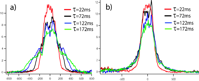
Figure 10: Longitudinal density profiles, each averaged over 10 realizations of the speckle pattern, observed after expansion times $\tau=$ 22, 72, 122 and 172 ms in a speckle potential of amplitude $\gamma=\sigma_{V}/\mu_{\rm{TF}}=0.3$ for: a) a quasi-1D potential ($\Delta y/R_{\rm{TF}}\simeq 3.5$) and b) a true 1D potential ($\Delta y/R_{\rm{TF}}\simeq 36$). In a), parabolic “wings”’ are visible around the central, trapped core. These continue to expand as a function of time.

In this article, we have presented a comparison of the expansion of a condensate in a 1D random potential with a theoretical scenario, obtaining good quantitative agreement. However, we have found that the 1D requirement for the potential is quite stringent. As described in section Section 2.3, we are able to vary both the size and anisotropy of the speckle grains. By performing the same experiments with a quasi-1D potential ($\Delta y/R_{\rm{TF}}\simeq 3.5$, as used in ref. [26]), we observe a behaviour on the longitudinal density profiles which is qualitatively different from that obtained using the true 1D potential ($\Delta y/R_{\rm{TF}}\simeq 36$) presented in this article.

The main difference is the appearance of “wings” in the longitudinal density profiles, which can be clearly seen in figure Figure 10(a). The shape of these wings is approximately an inverted parabola. Whereas the central core of the profile is trapped by the disorder, the wings continue to expand at a rate of 3.6(1) mm s^-1. This is significantly slower than condensate expansion in the absence of disorder, 6.1(1) mm s^-1. To exclude the possibility of these wings being composed of thermal atoms, produced by heating of the condensate in the speckle potential, we repeated the experiment with an atom cloud at 600 nK with a condensate fraction of only 15%. In this case, the large thermal fraction leads to wings with a gaussian profile, which expand with a velocity of 11(2) mm s^-1. From this we conclude that the additional wings appearing in the BEC during expansion in a quasi-1D random potential must be related to possibility of condensate atoms passing around some of the speckle peaks and continuing to expand.

The measurement of the rms size $L$ in quasi-1D potentials reveals the phenomenon of suppression of transport as $L$ saturates [26]. Yet, since the additional wings contribute to the rms size $L$ of the condensate, $L$ may continue to increase for some time after the onset of disorder-induced trapping of the central core and thus may not give a direct access to the time-scale of the trapping scenario. Therefore, in a quasi-1D potential, it is important to study the time evolution of the density profiles in order to correctly obtain the predicted timescales for this trapping phenomenon.

References

- [1] Glyde H R, Plantevin O, Fak B, Coddens G, Danielson P S and Schober S 2000 Phys. Rev. Lett. 84 2646
- [2] Dalichaouch R, Amstrong J P, Schultz S, Platzman P M and McCall S L 1991 Nature 354 53
- [3] Chabanov A A, Stoytchev M and Genack A Z 2000 Nature 404 850
- [4] Wiersma D S, Bartolini P, Lagendijk A and Righini R 1997 Nature 390 671
- [5] See for example Estève J, Aussibal C, Schumm T, Figl C, Mailly D, Bouchoule I, Westbrook C I and Aspect A 2004 Phys. Rev. A 70 043629 and references therein
- [6] Nagaoka Y and Fukuyama H (Eds.) 1982 Anderson Localization, Springer Series in Solid State Sciences 39 (Springer, Berlin, 1982); Ando T and Fukuyama H (Eds.) 1988 Anderson Localization, Springer Proceedings in Physics 28 (Springer, Berlin, 1988)
- [7] van Tiggelen B 1999 in Wave Diffusion in Complex Media, lectures notes at Les Houches 1998, edited by J. P. Fouque, NATO Science (Kluwer, Dordrecht, 1999)
- [8] Anderson P W 1958 Phys. Rev. 109 1492.
- [9] Mézard M, Parisi G and Virasoro M A 1987 Spin Glass Theory and Beyond (World Scientific, Singapour, 1987); Newman C M and Stein D L 2003 J. Phys.-Condens. Mat. 15 R1319; Sachdev S 1999 Quantum Phase Transitions, (Cambridge University Press, Cambridge, 1999)
- [10] Fisher M P A, Weichman P B, Grinstein G and Fisher D S 1989 Phys. Rev. B 40 546 ; Giamarchi T and Schulz H J 1988 Phys. Rev. B 37 4632
- [11] Dorokhov O N 1990 Sov. Phys. JETP 71 360; Shepelyansky D L 1994 Phys. Rev. Lett. 73 2607; Graham R and Pelster A cond-mat/0508306
- [12] Sanchez-Palencia L, Gangardt D M, Bouyer P, Shlyapnikov G V and Aspect A 2006 in preparation
- [13] Damski B, Zakrzewski J, Santos L, Zoller P and Lewenstein M 2003 Phys. Rev. Lett. 91 080403
- [14] Gavish U and Castin Y 2005 Phys. Rev. Lett. 95 020401
- [15] De Martino A, Thorwart M, Egger R and Graham R 2005 Phys. Rev. Lett. 94 060402
- [16] Sanchez-Palencia L and Santos L 2005 Phys. Rev. A 72 053607
- [17] Roth R and Burnett K 2003 J. Opt. B Quantum Semiclassical Opt. 5 S50
- [18] Fallani L, Lye J E, Guarrera V, Fort C and Inguscio M 2006 cond-mat/0603655
- [19] Sanpera A, Kantian A, Sanchez-Palencia L, Zakrzewski J and Lewenstein M 2004 Phys. Rev. Lett. 93 040401; see also Sanchez-Palencia L, Ahunfinger V, Kantian A, Zakrzewski J, Sanpera A and Lewenstein M 2006 J. Phys. B: At. Mol. Opt. Phys. 39 S121-S134
- [20] Ahufinger V, Sanchez-Palencia L, Kantian A, Sanpera A and Lewenstein M 2005 Phys. Rev. A 72 063616
- [21] For recent a review, see Anglin J R and Ketterle W 2002 Nature 416 211
- [22] private communication, Zoller P, Büchler H P and Bloch I; see also Ref. [14].
- [23] Horak P, Courtois J-Y and Grynberg G 1998 Phys. Rev. A 58 3953
- [24] Guidoni L, Triché C, Verkerk P and Grynberg G 1997 Phys. Rev. Lett. 79 3363; Guidoni L, Dépret P, di Stefano A and P. Verkerk 1999 Phys. Rev. A 60 R4233
- [25] Lye J E, Fallani L, Modugno M, Wiersma D, Fort C and Inguscio M 2005 Phys. Rev. Lett. 95 070401
- [26] Clément D, Varón A F, Hugbart M, Retter J A, Bouyer P, Sanchez-Palencia L, Gangardt D M, Shlyapnikov G V and Aspect A 2005 Phys. Rev. Lett. 95 170409
- [27] Fort C, Fallani L, Guarrera V, Lye J E, Modugno M, Wiersma D S and Inguscio M 2005 Phys. Rev. Lett. 95 170410
- [28] Schulte T, Drenkelforth S, Kruse J, Ertmer W, Arlt J, Sacha K, Zakrzewski J and Lewenstein M 2005 Phys. Rev. Lett. 95 170411
- [29] Goodman J W Speckle Phenomena: Theory and Applications preprint available at and Goodman J W 1975 in Laser speckle and related phenomena, edited by J.-C. Dainty (Springer-Verlag, Berlin, 1975)
- [30] Françon M 1978 La Granularité Laser (speckle) et ses applications en optique (Masson, Paris 1978)
- [31] Goodman J W 1985 Statistical Optics (Wiley-Interscience, 1985)
- [32] Lifshits I M, Gredeskul S A and Pastur L A 1988 Introduction to the theory of disordered systems (edited by Wiley-Interscience Publication, 1988)
- [33] Boyer V, Murdoch S, Le Coq Y, Delannoy G, Bouyer P and Aspect A 2000 Phys. Rev. A 62 021601(R)
- [34] Kagan Yu, Surkov E L and Shlyapnikok G V 1996 Phys. Rev. A 54 R1753; Castin Y and Dum R 1996 Phys. Rev. Lett. 77 5315