Electronic states near a quantum fluctuating point vortex in a $d$-wave superconductor: Dirac fermion theory

Abstract

We introduce a simple model of the low energy electronic states in the vicinity of a vortex undergoing quantum zero-point motion in a $d$-wave superconductor. The vortex is treated as a point flux tube, carrying $\pi$ flux of an auxiliary U(1) gauge field, which executes simple harmonic motion in a pinning potential. The nodal Bogoliubov quasiparticles are represented by Dirac fermions with unit U(1) gauge charge. The energy dependence of the local density of electronic states (LDOS) at the vortex center has no zero bias peak; instead, small satellite features appear, driven by transitions between different vortex eigenmodes. These results are qualitatively consistent with scanning tunneling microscopy measurements of the sub-gap LDOS in cuprate superconductors. Furthermore, as argued in L. Balents et al., Phys. Rev. B 71, 144508 (2005), the zero-point vortex motion also leads naturally to the observed periodic modulations in the spatial dependence of the sub-gap LDOS.

I Introduction

In a recent paper LorenzLDOS , hereafter referred to as I, two of the present authors considered influence of the vortex zero-point motion on the energy dependence of local density of electronic states (LDOS) in a $s$-wave superconductor. Here we will present a study of vortex zero point motion in two-dimensional $d$-wave superconductors, with an eye to application to the cuprate supercondcutors. A direct application of the methods of paper I to $d$-wave superconductors is discussed in Appendix C, but this approach has significant limitations. It makes a gradient expansion in the spatial dependence of the gap function and so cannot be applied in the limit of small coherence length, and is not designed to efficiently extract the important effects of the low-energy nodal quasiparticles. The body of the present paper will describe a new approach which overcomes these limitations.

Our focus on the zero-point motion of vortices in the cuprates is motivated by a previous proposal that periodic modulations in the spatial dependence of the LDOS inevitably appear over the region the vortex executes its quantum zero-point motion CompOrd1 ; VorMass . Such periodic LDOS modulations have been observed in scanning tunneling microscopy (STM) studies of the vortex in the cuprate superconductors hoffman ; fischer . Here we study whether the vortex motion could also explain the energy dependence of the LDOS near the vortex core.

A solution of the Bogoliubov-de Gennes (BdG) equations for a vortex in a $d$-wave superconductor leads to a large peak, as a function of energy, at zero bias at the vortex center Wang95 ; machida ; Franz98 . No such peak is observed in the experiments. The inclusion of additional density wave orders ting ; ghosal can suppress the zero bias peak in favor of spectral weight at satellites, but only under conditions in which the strength of the order parameter is unacceptably large. The theories require nearly complete magnetic/charge ordering, and there is no indication from e.g. neutron scattering experiments that such a large ordering can be present in the optimally doped Bi-based cuprates.

Paper I extended the BdG equations to include vortex zero-point motion for $s$-wave superconductors: it found that zero bias peak was reduced (but not eliminated), with a transfer of spectral weight to energies of order the vortex oscillation frequency. This was done in an approach that performed a gradient expansion in the gap function, which is only valid for a large core size.

The present paper examines an alternative approach to computing the sub-gap energy dependence of the LDOS near the vortex. Our starting point is an observation by Tsuchiura et al. ogata that the zero bias peak disappears when the vortex core size becomes of order the inverse Fermi wavevector. Consequently, we will examine a continuum model in which the vortex core becomes point-like, with a vanishing radius. In this situation, no gradient expansion can be performed, and it is essential to compute the effects of vortex zero-point motion without expanding in powers of the vortex position. We will demonstrate, within the context of a simple model, that not only is the zero-bias peak eliminated, but the vortex motion leads to satellite features associated with transitions between different vortex vibrational states. We will argue that these features are appealing candidates for explaining the sub-gap peaks observed in STM experiments aprile ; pan ; hoogen ; hoffman ; fischer .

In a sense, the analysis of this paper can be viewed as a method of computing the influence of “phase fluctuations”phase on the LDOS. However, instead of explicitly integrating over the phase degrees of freedom, we represent them by a collective co-ordinate, the position of the vortex. Apart from the benefit of the compact representation, this allows us to physically interpret the coupling of the phase fluctuations to the electronic quasiparticles. Furthermore, inclusion of Aharanov-Bohm phase factors exposes the subtle relationship of the vortex fluctuations to competing order parameters CompOrd1 .

The outline of the paper is as follows. Our model will be introduced in Section II, along with an initial discussion of its characteristic properties. The details of our calculations are presented in Section III. After setting up the formalism, we first analyze the LDOS influenced only by the vortex zero-point quantum motion, and then include the resonant scattering at the lowest order of perturbation theory. Plots of the full LDOS are shown in the Sections III.3 and III.4. We summarize our results and their relation to experiments in Section IV.

II The model

We consider a single vortex coupled to quasiparticles in a clean $d$-wave superconductor at zero temperature. The vortex is assumed to experience a harmonic trapping potential in which it can carry out its quantum zero-point motion. Such a potential can result from interactions between vortices in a vortex lattice, or from a pinning impurity. The Hamiltonian can be written as ($\hbar=1$):

$$H = \frac{\boldsymbol{p}_{\textrm{v}}^{2}}{2m_{\textrm{v}}}+\frac{1}{2}m_{\textrm{v}}\omega_{\textrm{v}}^{2}\boldsymbol{r}_{\textrm{v}}^{2}$$ (1)

$$~{}~{}~{}~{}+\sum_{\textrm{nodes}}\int\textrm{d}^{2}r\Psi^{\dagger}(\boldsymbol{r})H_{BdG}(\boldsymbol{r})\Psi^{\phantom{\dagger}}(\boldsymbol{r})\ .$$

For now we neglect the Magnus force on the vortex, assuming that it is much smaller that the trapping force; we shall consider it carefully in the Section III.4. The operators $\boldsymbol{p}_{\textrm{v}}$ and $\boldsymbol{r}_{\textrm{v}}$ are the canonical momentum and position of the vortex. For simplicity, we place the vortex in an isotropic trap characterized by a single harmonic frequency $\omega_{\textrm{v}}$. It has been shown that presence of static vortices does not qualitatively change the low-energy spectrum of nodal $d$-wave quasiparticles Franz98 ; Tesh1 ; Tesh2 , and in this paper we will find that the gapless nodes also survive quantum fluctuations of vortices. Therefore, quasiparticles are massless Dirac spinors and we describe them by Nambu operators $\Psi^{\dagger}(\boldsymbol{r})$ and $\Psi(\boldsymbol{r})$ defined at every node in the $d$-wave spectrum. Being interested only in the low-energy dynamics, we linearize the Bogoliubov-de Gennes Hamiltonian in the vicinity of gap-nodes, and apply a convenient Franz-Tešanović unitary transformation. For the node $\boldsymbol{p}\approx k_{\textrm{f}}\hat{\boldsymbol{x}}$ we have Tesh1 ; Tesh2 :

$$H_{\textrm{BdG}}=v_{\textrm{f}}(p_{x}+a_{x})\sigma^{z}+v_{\Delta}(p_{y}+a_{y})\sigma^{x}+mv_{\textrm{f}}v_{x}I\ ,$$ (2)

and we need not explicitly worry about the other nodes because their linearized Hamiltonians are related by unitary transformations. Note that we formally work with $d_{xy}$ symmetry, which is related to $d_{x^{2}-y^{2}}$ by a rotation. In this expression, $\boldsymbol{p}$ is the quasiparticle momentum operator relative to the node, $m$ is the electron mass, $v_{\textrm{f}}$ and $v_{\Delta}$ are the Fermi and gap velocities respectively, and $\sigma^{\mu}$ are Pauli matrices. The effective gauge field $\boldsymbol{a}$ is proportional to the phase gradient of the superconducting order parameter, and thus corresponds to the $\pi$-flux centered at the vortex location. The role of $\boldsymbol{a}$ is to implement the statistical interaction between vortices and quasiparticles, so that when a quasiparticle completes a circle around the vortex its wavefunction changes sign. The supercurrent velocity field $\boldsymbol{v}$ appears in the Hamiltonian because the supercurrents that circulate around the vortex give rise to Doppler shifts of quasiparticle energies. Note, however, that only the projection of $\boldsymbol{v}$ on the nodal direction matters, and also that Doppler shift effects decrease rapidly beyond the London penetration depth from the vortex center.

Our goal is to elucidate only the qualitative features of quasiparticle spectra in the vicinity of a fluctuating vortex. Hence, we will make several simplifications that are not quantitatively justified in realistic situations, but the obtained spectra will nevertheless be remarkably similar to the spectra observed in experiments. The complexity of calculations is considerably reduced if the Doppler shift and all effects of anisotropy are neglected. The Bogoliubov-de Gennes Hamiltonian near the node $\boldsymbol{p}\approx\pm k_{\textrm{f}}\hat{\boldsymbol{x}}$ becomes:

$$H_{BdG}=\left(\begin{array}[]{cc}p_{x}+a_{x}&p_{y}+a_{y}\\ p_{y}+a_{y}&-(p_{x}+a_{x})\end{array}\right)\ ,$$ (3)

where we have set $v_{\textrm{f}}$ and $v_{\Delta}$ to unity. We will work in the units $\hbar=v_{\textrm{f}}=1$ at all times, except when we discuss scales.

The coupling between the fermions and the vortex arises from the gauge field. This is specified by the instantaneous position operator $\boldsymbol{r}_{\textrm{v}}$ of the vortex:

$$\boldsymbol{a}(\boldsymbol{r},\boldsymbol{r}_{\textrm{v}})=\frac{\hat{\boldsymbol{z}}\times(\boldsymbol{r}-\boldsymbol{r}_{\textrm{v}})}{2|\boldsymbol{r}-\boldsymbol{r}_{\textrm{v}}|^{2}}\ ,$$ (4)

assuming that we can regard the vortex core to be negligibly small.

The physical reason for these simplifications comes from our expectation that it is the vortex quantum fluctuations that produce the sub-gap peaks at about 7 meV from the Fermi level in the quasiparticle density of states aprile ; pan ; hoogen . Even if we regard the core of a static vortex to be infinitely small, as was done in the expression  (4), the zero-point quantum motion of the vortex in the harmonic trap creates a finite central region in which the supercurrents are gradually suppressed. The circulating superflow is then the strongest at some finite radius. Quasiparticles can scatter from this supercurrent distribution through any number of virtual excited states of the oscillating vortex. The result is a weak resonant state, a metastable binding between the vortex and a quasiparticle. In our simplified calculation this effect is solely due to the electron Berry phase, but the Doppler shift should also contribute it, even more directly as a partially attractive potential. Indeed, our calculation will qualitatively reproduce the sub-gap peaks in the density of states, which are reminiscent of a localized metastable state in the vortex core, and in our model originate from resonant scattering. In the light of this scenario, we do not expect anisotropies to play a qualitatively significant role. The Doppler shift may be important in enhancing these effects, but the mere demonstration of the sub-gap peaks through the Berry phase alone makes the case for relevance of the vortex quantum motion. Another possible mechanism is resonant scattering from the conventional vortex core, where the superconducting order parameter magnitude is suppressed. However, in $d$-wave superconductors the core is very small (a few lattice spacings), so that the corresponding resonance would occur only at relatively large energy. Note that we are not considering the possibility of bound core states: all quasiparticle states are expected to be extended in pure $d$-wave superconductors, even in the presence of vortices Franz98 ; Tesh1 ; Tesh2 .

Our main result is the quasiparticle local density of states (LDOS) in the vicinity of a quantum oscillating vortex. We calculate the LDOS perturbatively, using

$$\alpha=\left(\frac{m_{\textrm{v}}v_{\textrm{f}}^{2}}{\hbar\omega_{\textrm{v}}}\right)^{\frac{1}{2}}$$ (5)

as a small dimensionless parameter. We treat the vortex effective mass $m_{\textrm{v}}$ as an independent quantity, although it can be determined microscopically DWVorAct . After all simplifications, we can write the LDOS as the following scaling function of energy $\epsilon$ and distance $r$ from the origin (center of the vortex trap):

$$\rho(\epsilon,r)=\frac{\omega_{\textrm{v}}}{\hbar v_{\textrm{f}}^{2}}\sum_{n=0}^{\infty}\alpha^{2n}F_{n}\left(\frac{\epsilon}{\hbar\omega_{\textrm{v}}},\frac{\epsilon r}{\hbar v_{\textrm{f}}};\alpha\right)\ .$$ (6)

The universal functions $F_{n}(x,y;\alpha)$ can be regarded as being of the same order of magnitude for any given finite arguments. Note, however, that this is not a Taylor expansion. The extra dependence of $F_{n}$ on $\alpha$ is a somewhat unusual consequence of the proper choice of perturbation. It is usual to start from a non-interacting theory and include all interactions as perturbations. Unfortunately, interactions between quasiparticles and vortices are not weak, and cannot be characterized by a small expansion parameter. Instead, it is better to include the influence of the vortex zero-point quantum motion on quasiparticles at the zeroth order, and treat the resonant scattering of quasiparticles from the oscillating vortex as a perturbation. Thus we perform a partial resummation of the $\alpha$ expansion, and this accounts for the $\alpha$ dependence of the co-efficients in Eq. (6); features of the zero-point vortex motion, also parameterized by $\alpha$, appear in the LDOS at all orders of perturbation theory. The small parameter $\alpha$ is the ratio of such perturbation’s energy scale and the energy barrier $\hbar\omega_{\textrm{v}}$ for virtual transitions.

As a matter of fact, only the zero-point vortex oscillations set the scale for the zeroth order term in  (6), which results in an additional scaling property of $F_{0}(x,y;\alpha)$:

$$F_{0}(x,y;\alpha)=\alpha F_{0}(x/\alpha,y;1)\ .$$ (7)

One should not be misled to conclude that $F_{0}$ becomes small when $\alpha\to 0$: as we will show, $F_{0}(x,y;\alpha)\to x/(2\pi)$ for $x\gg\alpha$.

III Perturbation theory

The Hamiltonian  (1) can be expressed in a fashion analogous to the Holstein-Primakoff expansion for the spin systems. In absence of quasiparticles the vortex is modeled by a two-dimensional linear harmonic oscillator, whose eigenstates $|n_{x},n_{y}\rangle$ are characterized by two integer quantum numbers, $n_{x}$ and $n_{y}$. Let us define the following “matrix elements”:

$$V_{(n_{1x},n_{1y}),(n_{2x},n_{2y})}(\boldsymbol{r})=\langle n_{1x},n_{1y}|H_{BdG}(\boldsymbol{r})|n_{2x},n_{2y}\rangle\ .$$ (8)

We also introduce creation operators, $b_{x}^{\dagger}$ and $b_{y}^{\dagger}$, which raise the vortex quantum number:

$$b_{x}^{\dagger}|n_{x},n_{y}\rangle=\sqrt{n_{x}+1}|n_{x}+1,n_{y}\rangle,$$ (9)

and similarly for $b_{y}^{\dagger}$. If we insert the identity operators on the left and right side of $H_{BdG}$ in the equation  (1), and resolve them in terms of the vortex eigenstates $|n_{x},n_{y}\rangle$, we can systematically write:

$$\Psi^{\dagger}H_{BdG}\Psi^{\phantom{\dagger}}=\Psi^{\dagger}\Bigl{\{}V_{(0,0),(0,0)}+$$ (10)

$$~{}~{}~{}~{}~{}V_{(1,0),(0,0)}b_{x}^{\dagger}+h.c.+V_{(0,1),(0,0)}b_{y}^{\dagger}+h.c.+$$

$$~{}~{}~{}~{}~{}\left(V_{(1,0),(1,0)}-V_{(0,0),(0,0)}\right)b_{x}^{\dagger}b_{x}^{\phantom{\dagger}}+$$

$$~{}~{}~{}~{}~{}\left(V_{(0,1),(0,1)}-V_{(0,0),(0,0)}\right)b_{y}^{\dagger}b_{y}^{\phantom{\dagger}}+$$

$$~{}~{}~{}~{}~{}V_{(1,0),(0,1)}b_{x}^{\dagger}b_{y}^{\phantom{\dagger}}+h.c.+V_{(1,1),(0,0)}b_{x}^{\dagger}b_{y}^{\dagger}+h.c.+$$

$$~{}~{}~{}~{}~{}\frac{1}{\sqrt{2}}V_{(2,0),(0,0)}b_{x}^{\dagger}b_{x}^{\dagger}+h.c.+$$

$$~{}~{}~{}~{}~{}\frac{1}{\sqrt{2}}V_{(0,2),(0,0)}b_{y}^{\dagger}b_{y}^{\dagger}+h.c.+\cdots\Bigr{\}}\Psi^{\phantom{\dagger}}\ .$$

It can be easily seen that the quasiparticle momentum operators $\boldsymbol{p}$ appear only in the lowest order term $V_{(0,0),(0,0)}$. In all elastic processes (such as $b_{x}^{\dagger}b_{x}^{\phantom{\dagger}}$) the momentum operators that appear in the matrix elements $V$ are cancelled out. On the other hand, in all inelastic processes the momentum operators do not appear because they do not excite vortex states. Therefore, for practical purposes we can replace all matrix elements except $V_{(0,0),(0,0)}$ with:

$$V_{(n_{1x},n_{1y}),(n_{2x},n_{2y})}(\boldsymbol{r})=\left(\begin{array}[]{cc}a_{x}^{\prime}(\boldsymbol{r})&a_{y}^{\prime}(\boldsymbol{r})\\ a_{y}^{\prime}(\boldsymbol{r})&-a_{x}^{\prime}(\boldsymbol{r})\end{array}\right)\ ,$$ (11)

where

$$\boldsymbol{a}^{\prime}(\boldsymbol{r}) \equiv \boldsymbol{a}_{(n_{1x},n_{1y}),(n_{2x},n_{2y})}(\boldsymbol{r})$$

$$= \langle n_{1x},n_{1y}|\boldsymbol{a}(\boldsymbol{r},\boldsymbol{r}_{\textrm{v}})|n_{2x},n_{2y}\rangle\ .$$

Note that the bare effective gauge field $\boldsymbol{a}(\boldsymbol{r},\boldsymbol{r}_{\textrm{v}})$, given by  (4), does not define any energy or length scale. The scales are introduced through the states $|n_{x},n_{y}\rangle$ of the quantum harmonic oscillator. The harmonic oscillator wavefunctions depend only on the dimensionless coordinates $\boldsymbol{\xi}=\sqrt{m_{\textrm{v}}\omega_{\textrm{v}}}\boldsymbol{r}$, so that the energy scale associated with $V_{(n_{1x},n_{1y}),(n_{2x},n_{2y})}$ is $(\hbar\omega_{\textrm{v}}m_{\textrm{v}}v_{\textrm{f}}^{2})^{1/2}$ (when all physical constants are put in their places).

The expansion  (10) separates various processes in which quasiparticles can scatter elastically or inelastically from a vortex. At low enough energies the expansion can be truncated after a few lowest order terms. In the following we will set up a perturbation theory, with the unperturbed Hamiltonian:

$$H_{0}=\omega_{\textrm{v}}\left(b_{x}^{\dagger}b_{x}^{\phantom{\dagger}}+b_{y}^{\dagger}b_{y}^{\phantom{\dagger}}\right)+\int\textrm{d}^{2}r\Psi^{\dagger}V_{(0,0),(0,0)}\Psi^{\phantom{\dagger}}\ ,$$ (13)

and the perturbation:

$$H_{1}=\int\textrm{d}^{2}r\Psi^{\dagger}\left(V_{(1,0),(0,0)}b_{x}^{\dagger}+V_{(0,1),(0,0)}b_{y}^{\dagger}+h.c.\right)\Psi^{\phantom{\dagger}}\ .$$ (14)

The more complicated scattering processes in  (10) become qualitatively important only at energies $\epsilon\sim 2\omega_{\textrm{v}}$ and above.

Before we begin calculations, it is useful to identify the small parameter of the perturbation theory. The available parameters in the model  (1) define two energy scales: the energy of vortex quantum oscillations $\hbar\omega_{\textrm{v}}$, and the characteristic kinetic energy $m_{\textrm{v}}v_{\textrm{f}}^{2}$. The unperturbed Hamiltonian  (13) is properly characterized by the scale $|H_{0}|=\hbar\omega_{\textrm{v}}$, because the vortex harmonic frequency sets the energy barrier that needs to be crossed in perturbative virtual transitions. The energy scale of the perturbation  (14) is $|H_{1}|=(\hbar\omega_{\textrm{v}}m_{\textrm{v}}v_{\textrm{f}}^{2})^{1/2}$, as discussed above. Therefore, we can define the small parameter $\alpha=|H_{1}|/|H_{0}|$ given by expression  (5). The lowest order correction $\rho_{1}$ to the quasiparticle LDOS comes from the Fock exchange process (self-energy), so that $\rho_{1}\propto\alpha^{2}$. Namely, every vertex $\propto|H_{1}|$ in Feynman diagrams introduces a factor of $\alpha$, which becomes apparent after rescaling all energies by $|H_{0}|=\hbar\omega_{\textrm{v}}$ as was done in  (6).

In practice, one also has to keep in mind the quasiparticle cut-off energy $\Lambda$. This third energy scale physically comes from the superconducting gap amplitude, beyond which linearization of the Bogoliubov-de Gennes Hamiltonian breaks down. Furthermore, renormalization of the effective vortex mass due to quasiparticles DWVorAct is such that $m_{\textrm{v}}v_{\textrm{f}}^{2}\sim\Lambda$. Irrespective of its physical origin, numerical analysis requires that $\Lambda$ be introduced. However, in the ideal linearized model that we are concerned with, we can in principle take the $\Lambda\to\infty$ limit. As long as we treat the vortex mass $m_{\textrm{v}}$ and frequency $\omega_{\textrm{v}}$ as independent parameters, we find that the spectrum does not depend on the numerically introduced $\Lambda$ at energies sufficiently below $\Lambda$. The functions $F_{n}$ in  (6) are universal.

III.1 The LDOS due to vortex zero-point quantum motion

We begin by considering the lowest order term in the expansion  (6) for the LDOS:

$$\rho_{0}(\epsilon,r)=\frac{\omega_{\textrm{v}}}{\hbar v_{\textrm{f}}^{2}}F_{0}\left(\frac{\epsilon}{\hbar\omega_{\textrm{v}}},\frac{\epsilon r}{\hbar v_{\textrm{f}}};\alpha\right)\ .$$ (15)

This term contains effects of the vortex zero-point quantum motion on quasiparticle spectra, but excludes effects of the resonant scattering. For this purpose we will numerically diagonalize the Hamiltonian  (13) in infinite space.

It will be useful to first understand the solution for a static vortex, which is obtained in the limit of $m_{\textrm{v}}\omega_{\textrm{v}}\to\infty$. In this limit there are no vortex fluctuations, so that $V_{(0,0),(0,0)}$ reduces to  (3), with the gauge field given by  (4), and $\boldsymbol{r}_{\textrm{v}}\equiv 0$. Exact analytical solutions (properly normalized in the infinite space) are then found to be DWVorAct :

$$\psi_{q,l,k}^{\infty}(r,\phi)=\sqrt{\frac{\epsilon}{4\pi}}\times$$ (16)

$$~{}~{}\left\{\begin{array}[]{lcl}\left(\begin{array}[]{c}J_{-l+\frac{1}{2}}(kr)e^{i(l-1)\phi}\\ -iq\cdot J_{-l-\frac{1}{2}}(kr)e^{il\phi}\end{array}\right)&\quad,&l\leq 0\\ \left(\begin{array}[]{c}J_{l-\frac{1}{2}}(kr)e^{i(l-1)\phi}\\ iq\cdot J_{l+\frac{1}{2}}(kr)e^{il\phi}\end{array}\right)&\quad,&l\geq 0\end{array}\right\}$$ (23)

in the representation that diagonalizes the angular momentum. Quasiparticles carry the following quantum numbers: “charge” $q=\pm 1$ (distinguishes particle-like and hole-like states), angular momentum $l\in\mathbb{Z}$ and radial wavevector $k>0$. There are only extended quasiparticle states with energies $\epsilon=q|k|$. $J_{l}(kr)$ are Bessel functions of the first kind. The wavefunction for $l=0$ is a linear combination of the two forms of $\psi_{q,0,k}^{\infty}$ in  (16), which can be uniquely specified only with a separate boundary condition at the vortex location (an artifact of $m_{\textrm{v}}\omega_{\textrm{v}}\to\infty$ and a point-like core) Tesh2 . The corresponding LDOS $\rho_{\infty}$ diverges as $1/r$ at any energy, due to the $l=0$ wavefunctions, which include $J_{-\frac{1}{2}}(kr)$:

$$\rho_{\infty}(\epsilon,r) = \frac{\cos(2|\epsilon|r)}{2\pi^{2}r}+\frac{|\epsilon|}{\pi}\sum_{l=0}^{\infty}J_{l+\frac{1}{2}}^{2}(|\epsilon|r)$$ (26)

$$\longrightarrow \left\{\begin{array}[]{c@{\quad, \quad}c}\frac{1}{2\pi^{2}r}&|\epsilon|r\ll 1\\[5.69054pt] \frac{|\epsilon|}{2\pi}&|\epsilon|r\gg 1\end{array}\right\}\ .$$

For finite $\omega_{\textrm{v}}$ and $m_{\textrm{v}}$ the vortex fluctuates in a finite region whose radius is $\sim(\omega_{\textrm{v}}m_{\textrm{v}})^{-1/2}$. This is a property of the harmonic oscillator ground-state. The exact quasiparticle eigenstates are still characterized by the same quantum numbers, and only the dependence on radius $r$ is changed. This is so because in the ground-state of our model the vortex wavefunction is rotationally symmetric, and well localized in a finite region of space. The LDOS $\rho_{0}$ affected only by vortex zero-point oscillations will coincide with  (26) at energies $\epsilon\gg(m_{\textrm{v}}\omega_{\textrm{v}})^{1/2}$ or distances $r\gg(m_{\textrm{v}}\omega_{\textrm{v}})^{-1/2}$.

The first step in diagonalizing  (13) is to calculate $V_{(0,0),(0,0)}$. From the definition  (8) we see that $V_{(0,0),(0,0)}$ is given by the expression  (3) with an effective “gauge field”:

$$\boldsymbol{a}_{(0,0),(0,0)}(\boldsymbol{r})=\langle 0,0|\boldsymbol{a}(\boldsymbol{r},\boldsymbol{r}_{\textrm{v}})|0,0\rangle\ ,$$ (27)

where $\boldsymbol{a}(\boldsymbol{r},\boldsymbol{r}_{\textrm{v}})$ is given by  (4). Substituting here the ground-state wavefunctions of the linear harmonic oscillator, we get:

$$\boldsymbol{a}_{(0,0),(0,0)}(\boldsymbol{r})=\left(1-e^{-m_{\textrm{v}}\omega_{\textrm{v}}r^{2}}\right)\boldsymbol{a}(\boldsymbol{r},0)\ .$$ (28)

Details of this derivation are presented in Appendix  A. The effective gauge field is not singular at the origin, even though the static vortex has a point-like core. This indicates that supercurrents are suppressed near the origin. Effectively, a “vortex core” has been created, and hence the exact wavefunctions are significantly modified from  (16). Behavior of the exact wavefunctions $\psi=(e^{i(l-1)\phi}u(r),e^{il\phi}v(r))$ at small $r$ becomes:

$$u(r)\propto J_{l-1}(\kappa_{l}r)\ ,$$ (29)

and similar for $v(r)$, where $\kappa_{l}=\sqrt{k^{2}-lm_{\textrm{v}}\omega_{\textrm{v}}}$. These wavefunctions are always finite or zero at the origin, so that the LDOS is not divergent. For $r\gg(\omega_{\textrm{v}}m_{\textrm{v}})^{-1/2}$ the exact wavefunctions reduce to the form given by  (16), except that there is a phase shift: $\psi(r,\phi)=\psi^{\infty}(r+\delta_{l,k},\phi)$. The known behavior for small and large $r$ allows one to easily find and normalize exact wavefunctions in infinite space: the radial Schrödinger equation is first numerically solved in a finite region of space $r<r_{0}$, and then the solution is matched by value and derivative to the phase shifted form  (16) for $r>r_{0}\gg(m_{\textrm{v}}\omega_{\textrm{v}})^{-1/2}$.

In the figure  1 we plot the LDOS $\rho_{0}(\epsilon)$ at the origin for several values of the dimensionless parameter $\alpha^{2}$. All plots collapse to a single curve (shown in the inset) if both the energy and LDOS are rescaled by $(m_{\textrm{v}}\omega_{\textrm{v}})^{1/2}$, because only this energy appears in the quasiparticle part of the Hamiltonian  (13). Hence, the following scaling applies:

$$\rho_{0}(\epsilon,r)=\frac{\sqrt{\hbar m_{\textrm{v}}\omega_{\textrm{v}}v_{\textrm{f}}^{2}}}{(\hbar v_{\textrm{f}})^{2}}F_{0}^{\prime}\left(\frac{\epsilon}{\sqrt{\hbar m_{\textrm{v}}\omega_{\textrm{v}}v_{\textrm{f}}^{2}}},\frac{\epsilon r}{\hbar v_{\textrm{f}}}\right)\ ,$$ (30)

which in comparison with  (15) implies:

$$F_{0}(x,y;\alpha)=\alpha F_{0}^{\prime}(x/\alpha,y)=\alpha F_{0}(x/\alpha,y;1)\ .$$ (31)

At large energies ($\epsilon\gg(m_{\textrm{v}}\omega_{\textrm{v}})^{1/2}$), the LDOS at the origin begins to reflect the bulk density of states, and hence becomes a linear function of energy. Furthermore, $\rho_{0}(\epsilon,r)$ in the bulk ($r\gg(m_{\textrm{v}}\omega_{\textrm{v}})^{-1/2}$) must coincide with $\rho_{\infty}(\epsilon,r)$ of the static vortex, so that the expression  (26) determines both the large energy and large distance behavior of $\rho_{0}(\epsilon,r)$:

$$F_{0}(x,y;\alpha)\to\frac{x}{2\pi}\quad,\quad\frac{x}{\alpha}\vee y\gg 1\ .$$ (32)

Spatial variations of the LDOS are illustrated in the figure  2. Zero-point quantum motion of the vortex removes the $1/r$ divergence of the LDOS found in the core of a static vortex, while at large distances quasiparticles do not feel the vortex fluctuations.

Figure 1: The quasiparticle LDOS influenced solely by the vortex zero-point quantum motion. The LDOS is plotted at the origin as a function of energy and $\alpha^{2}$. All plots can be rescaled to a single curve, shown in the inset.

Figure 2: The quasiparticle LDOS influenced solely by the vortex zero-point quantum motion, plotted at the energy $\epsilon=\omega_{\textrm{v}}$ as a function of distance $r$ from the origin. The solid and dashed lines correspond to an oscillating ($\alpha^{2}=5$), and a static vortex respectively. The apparent drop of LDOS for the oscillating vortex beyond $r\approx 4$ is an artifact of numerical calculation, which took into account only a small number of angular momentum channels ($-5\leq l\leq 5$).

Smallness of the vortex core, measured by the coherence length $\xi\ll(m_{\textrm{v}}\omega_{\textrm{v}})^{-1/2}$, seems to be responsible for absence of the zero-energy peak in the quasiparticle LDOS, as was suggested in the Ref.ogata, . This can be inferred by comparing the LDOS obtained here with the LDOS of a similar calculation from the Appendix C. The approach from the Appendix works in the opposite limit $\xi>(m_{\textrm{v}}\omega_{\textrm{v}})^{-1/2}$ and produces a broad zero-energy peak in the quasiparticle LDOS.

III.2 One-loop correction

In order to explore the resonant scattering of quasiparticles from the fluctuating vortex, we calculate the one-loop correction to the quasiparticle Green’s function. This will directly lead to the lowest order LDOS correction:

$$\rho_{1}(\epsilon,r)=\alpha^{2}\frac{\omega_{\textrm{v}}}{\hbar v_{\textrm{f}}^{2}}F_{1}\left(\frac{\epsilon}{\hbar\omega_{\textrm{v}}},\frac{\epsilon r}{\hbar v_{\textrm{f}}};\alpha\right)\ ,$$ (33)

which we will discuss in Section III.3

The Hamiltonian given by  (13) and  (14) defines a problem of massless Dirac fermions coupled to a single bosonic oscillator. The unperturbed fermion states are characterized by “charge” $q$, radial wavevector $k$ and angular momentum $l$. Perturbation theory can be visualized using the standard Feynman diagram technique. The bare propagators ($G_{0}$ for quasiparticles and $D_{0}^{\mu\nu}$ for the vortex) and vertices are:

$$\begin{array}[]{ccc}\includegraphics[width=57.81621pt]{propagator-fermion-labeled.eps}&&G_{0}(q,k,l,\omega)=\frac{1}{\omega-q(k-i0^{+})}\\ \includegraphics[width=57.81621pt]{propagator-vortex-labeled.eps}&&D_{0}^{\mu\nu}(\omega)=\frac{2\omega_{\textrm{v}}}{\omega^{2}-\omega_{\textrm{v}}^{2}+i0^{+}}\delta_{\mu\nu}\\ \begin{minipage}{72.26999pt} \includegraphics[width=72.26999pt]{vertex-labeled.eps} \end{minipage}&&V_{q_{1},l_{1},k_{1};q_{2},l_{2},k_{2}}^{\nu}\end{array}$$ (34)

Here, the indices $\mu$ and $\nu$ denote spatial directions $x$ and $y$, and summation over repeated indices will be assumed from now on. The vertex operator $V_{q_{1},l_{1},k_{1};q_{2},l_{2},k_{2}}^{\mu}$ is the Fourier transform of $V_{(1,0),(0,0)}=V_{(0,0),(1,0)}$ for $\mu=x$ and $V_{(0,1),(0,0)}=V_{(0,0),(0,1)}$ for $\mu=y$. Frequency is conserved at vertices, but $k$ and $l$ are not. Physical conservation of angular momentum is reflected by requirement that $V_{q_{1},l_{1},k_{1};q_{2},l_{2},k_{2}}^{\mu}\propto\delta_{|l_{1}-l_{2}|,1}$; the first excited states of the 2D harmonic oscillator carry angular momentum $l=\pm 1$, and in these inelastic scattering processes the quasiparticle angular momentum changes by one.

The one-loop self-energy $\Sigma$ has two contributions, in principle:

$$\begin{array}[]{ccc}\includegraphics[width=72.26999pt]{selfenergy-hartree-labeled.eps}&&\includegraphics[width=108.405pt]{selfenergy-fock-labeled.eps}\\ \textrm{Hartree}&&\textrm{Fock}\end{array}$$ (35)

The Hartree self-energy is zero within the present approximations because the vertex that touches the fermion loop has the same incoming and outgoing angular momentum. The Fock self-energy is:

$$\Sigma_{q_{1},l_{1},k_{1};q_{2},l_{2},k_{2}}(\omega)=i\sum_{q^{\prime},l^{\prime}}\int\textrm{d}k^{\prime}\frac{\textrm{d}\omega^{\prime}}{2\pi}G_{0}(q^{\prime},l^{\prime},k^{\prime},\omega^{\prime})$$

$$~{}~{}~{}\times D_{0}^{\mu\nu}(\omega-\omega^{\prime})V_{q_{1},l_{1},k_{1};q^{\prime},l^{\prime},k^{\prime}}^{\mu}V_{q^{\prime},l^{\prime},k^{\prime};q_{2},l_{2},k_{2}}^{\nu}$$

$$~{}~{}~{}=\sum_{q^{\prime},l^{\prime}}\int\textrm{d}k^{\prime}\frac{V_{q_{1},l_{1},k_{1};q^{\prime},l^{\prime},k^{\prime}}^{\mu}V_{q^{\prime},l^{\prime},k^{\prime};q_{2},l_{2},k_{2}}^{\mu}}{\omega-q^{\prime}(\omega_{\textrm{v}}+k^{\prime}-i0^{+})}\ .$$ (36)

The one-loop correction to the quasiparticle Green’s function is given by the simplest diagram that contains only one self-energy part:

$$G_{q_{1},l_{1},k_{1};q_{2},l_{2},k_{2}}^{(1)}(\omega)=$$ (37)

$$~{}~{}~{}~{}~{}G_{0}(q_{1},l_{1},k_{1},\omega)G_{0}(q_{2},l_{2},k_{2},\omega)\Sigma_{q_{1},l_{1},k_{1};q_{2},l_{2},k_{2}}(\omega)\ .$$

The remaining task is to calculate the vertex operators $V_{q_{1},l_{1},k_{1};q_{2},l_{2},k_{2}}^{\mu}$ in momentum space. In the original position representation these operators have the form  (11), where the first-order effective gauge fields $\boldsymbol{a}^{\mu}$ ($\mu\in\{x,y\}$) are:

$$\boldsymbol{a}^{x} = \langle 1,0|\boldsymbol{a}(\boldsymbol{r},\boldsymbol{r}_{\textrm{v}})|0,0\rangle=-\sqrt{\frac{m_{\textrm{v}}\omega_{\textrm{v}}}{2}}\times$$

$$\times \left[\frac{1-e^{-\xi^{2}}}{\xi^{2}}\hat{\boldsymbol{y}}+\frac{(1+\xi^{2})e^{-\xi^{2}}-1}{\xi^{2}}\cdot\frac{2\xi_{x}\hat{\boldsymbol{z}}\times\boldsymbol{\xi}}{\xi^{2}}\right]$$

$$\boldsymbol{a}^{y} = \langle 0,1|\boldsymbol{a}(\boldsymbol{r},\boldsymbol{r}_{\textrm{v}})|0,0\rangle=\sqrt{\frac{m_{\textrm{v}}\omega_{\textrm{v}}}{2}}\times$$

$$\times \left[\frac{1-e^{-\xi^{2}}}{\xi^{2}}\hat{\boldsymbol{x}}-\frac{(1+\xi^{2})e^{-\xi^{2}}-1}{\xi^{2}}\cdot\frac{2\xi_{y}\hat{\boldsymbol{z}}\times\boldsymbol{\xi}}{\xi^{2}}\right]\ .$$

Here, $\boldsymbol{\xi}=(\xi_{x},\xi_{y})$ are the usual dimensionless coordinates of the quantum harmonic oscillator, given by $\boldsymbol{\xi}=\sqrt{m_{\textrm{v}}\omega_{\textrm{v}}}\boldsymbol{r}$. For switching to the momentum representation it will be convenient to keep the spinor structure and organize various quantities into spinor matrices. The role of spin $s$ is taken over by the quantum number $q$ in the momentum representation, which can take only two values being the sign of energy. First, we define the Fourier weight matrix, which is used to translate between the position and momentum representations:

$$T_{l,k}(\boldsymbol{r})=\left(\begin{array}[]{cc}u_{+,l,k}(\boldsymbol{r})&u_{-,l,k}(\boldsymbol{r})\\ v_{+,l,k}(\boldsymbol{r})&v_{-,l,k}(\boldsymbol{r})\end{array}\right)\ .$$ (39)

This matrix is expressed in terms of the eigenfunctions of the unperturbed Hamiltonian  (13), which in the position representation look like:

$$\psi_{q,k,l}(\boldsymbol{r})=\left(\begin{array}[]{c}u_{q,l,k}(\boldsymbol{r})\\ v_{q,l,k}(\boldsymbol{r})\end{array}\right)\ .$$ (40)

The quasiparticle spinor operators in position and momentum representations are related by:

$$\Psi(\boldsymbol{r})=\sum_{l}\int\textrm{d}kT_{l,k}(\boldsymbol{r})\Psi_{l,k}\ .$$ (41)

In the momentum representation, the bare quasiparticle propagator is of course diagonal:

$$G_{0}(k,l,\omega)=\left(\begin{array}[]{cc}\frac{1}{\omega-k+i0^{+}}&0\\ 0&\frac{1}{\omega+k-i0^{+}}\end{array}\right)\ .$$ (42)

The momentum representation of the vertex operators is obtained in the following manner:

$$V_{l_{1},k_{1};l_{2},k_{2}}^{\mu}=\int\textrm{d}^{2}rT_{l_{1},k_{1}}^{\dagger}(\boldsymbol{r})V^{\mu}(\boldsymbol{r})T_{l_{2},k_{2}}^{\phantom{\dagger}}(\boldsymbol{r})\ ,$$ (43)

where $V^{\mu}(\boldsymbol{r})$ is either $V_{(1,0),(0,0)}$ or $V_{(0,1),(0,0)}$ depending on $\mu$. When  (11) and  (III.2) are substituted in this expression, it is possible to exactly integrate out the azimuthal angle $\phi$. This implements the physical angular momentum conservation, so that $V_{l_{1},k_{1};l_{2},k_{2}}^{\mu}=0$ unless $|l_{1}-l_{2}|=1$.

III.3 The LDOS due to resonant scattering

The local density of states is naturally obtained from the quasiparticle Green’s function. Including the quasiparticles at given position and energy of either spin and angular momentum gives the following expression in the spinor momentum representation:

$$\rho(\epsilon,\boldsymbol{r}) = -\frac{1}{\pi}\textrm{sign}(\epsilon)\cdot\textrm{Im}\Biggl{\{}\sum_{l_{1},l_{2}}\int\textrm{d}k_{1}\textrm{d}k_{2}$$

$$\textrm{Tr}\Bigl{[}T_{l_{1},k_{1}}^{\phantom{\dagger}}(\boldsymbol{r})G_{l_{1},k_{1};l_{2},k_{2}}(\epsilon)T_{l_{2},k_{2}}^{\dagger}(\boldsymbol{r})\Bigr{]}\Biggr{\}}\ .$$

In the absence of perturbations, we would substitute here the bare Green’s function $G_{0}$ from  (42). It is easy to show that the zeroth order term in the LDOS is:

$$\rho_{0}(\epsilon,\boldsymbol{r})=\sum_{l}\Bigl{\{}\left(|u_{+,l,|\epsilon|}(\boldsymbol{r})|^{2}+|v_{+,l,|\epsilon|}(\boldsymbol{r})|^{2}\right)\Theta(\epsilon)$$

$$~{}~{}~{}~{}~{}+\left(|u_{-,l,|\epsilon|}(\boldsymbol{r})|^{2}+|v_{-,l,|\epsilon|}(\boldsymbol{r})|^{2}\right)\Theta(-\epsilon)\Bigr{\}}\ .$$ (45)

This is the expected result, which could have been immediately written from the known eigenfunctions  (40); it is plotted as a function of energy in the figure  1.

The one-loop correction $\rho_{1}(\epsilon,\boldsymbol{r})$ to LDOS is found by substituting  (37) into  (III.3). The correction to the Green’s function is written in the spinor representation as:

$$G_{l_{1},k_{1};l_{2},k_{2}}^{(1)}(\omega)=G_{0}(l_{1},k_{1},\omega)\Sigma_{l_{1},k_{1};l_{2},k_{2}}(\omega)G_{0}(l_{2},k_{2},\omega)\ ,$$ (46)

where the self-energy matrix is:

$$\Sigma_{l_{1},k_{1};l_{2},k_{2}}(\omega)=\sum_{l}\int\textrm{d}k$$ (47)

$$~{}~{}~{}~{}~{}V^{\mu}_{l_{1},k_{1};l,k}\left(\begin{array}[]{cc}\frac{1}{\omega-k-\omega_{\textrm{v}}+i0^{+}}&0\\ 0&\frac{1}{\omega+k+\omega_{\textrm{v}}-i0^{+}}\end{array}\right)V^{\mu}_{l,k;l_{2},k_{2}}\ .$$ (50)

Details of the expression for LDOS and numerical procedures are elaborated in Appendix  B.

Figure 3: The one-loop correction $\rho_{1}$ to LDOS at the vortex center as a function of energy. These plots show evolution of $\rho_{1}(\epsilon)$ as the small parameter $\alpha^{2}$ changes. The magnitude of $\rho_{1}$ scales as $\alpha^{2}$. Quasiparticle cut-off energy is $\Lambda=4\omega_{\textrm{v}}$.

The one-loop correction to LDOS at the vortex center is plotted in the figure  3 as a function of energy. Some general features can be immediately noted. There is a discontinuity of LDOS when the quasiparticle energy is equal to the vortex harmonic frequency, $\epsilon=\omega_{\textrm{v}}$. Also, for all values of the small parameter $\alpha^{2}$, the LDOS has a local minimum at zero energy and grows into a peak at some finite energy. This feature could be interpreted as formation of a weak metastable state inside the spatial region spanned by the vortex quantum oscillations. Note that the LDOS peak shifts toward lower energies as $\alpha^{2}\propto m_{\textrm{v}}$ decreases: for smaller vortex mass $m_{\textrm{v}}$ the vortex oscillates in a larger region and hence tries to localize quasiparticles at lower energies. For very small values of $\alpha^{2}$ some additional features develop in the LDOS, such as secondary peaks and dips. It is possible that the values $\alpha^{2}\propto 1/n^{2}$ for integer $n$ are special and control appearance of various LDOS features (the plots hint to this possibility, but are not entirely conclusive). Physically, $\alpha$ is the ratio of two length scales: the quasiparticle wave-length at the energy $\epsilon=\omega_{\textrm{v}}$, and the spatial extent of the vortex zero-point quantum oscillations (effective core radius). Roughly speaking, features of the LDOS change qualitatively when the effective core region grows to enclose an additional quasiparticle wavelength $1/\omega_{\textrm{v}}$.

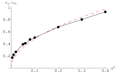
Figure 4: (color online) Energy $\epsilon_{c}$ of the sub-gap peak in the LDOS as a function of the small parameter $\alpha^{2}$, and the fit to $\epsilon_{c}\propto\alpha$ (red dashed). $\epsilon_{c}$ is defined as the energy of the first local maximum in $\rho_{1}(\epsilon)$ from the figure  3.

In the figure  4 we plot energy $\epsilon_{c}$ of the LDOS sub-gap peak as a function of $\alpha^{2}$. The peak position scales as energy of the perturbation that creates it: $\epsilon_{c}\propto\alpha\omega_{\textrm{v}}$. In order to see how this result relates to experimental observations, we will explore a somewhat different scenario. Suppose that the plot in the figure  4 were linear, so that $\epsilon_{c}/\omega_{\textrm{v}}$ were proportional to $\alpha^{2}$. This would mean that the sub-gap peak energy $\epsilon_{c}$ were proportional to $m_{\textrm{v}}v_{\textrm{f}}^{2}$ (see equation  (5)). It has been argued DWVorAct that the nodal quasiparticles renormalize the vortex mass $m_{\textrm{v}}$ to a value that is proportional to the superconducting gap amplitude $\Delta_{0}$. This renormalization due to quasiparticles is, likely, the largest contribution to the effective vortex mass, since the usual logarithmic infra-red divergence of the hydrodynamic vortex mass is cut-off by the Coulomb screening. Therefore, according to this scenario, $\epsilon_{c}\propto\Delta_{0}$. STM measurements are consistent with such linear scaling of the sub-gap peak energy with the superconducting gap amplitude. Most notably, the sub-gap peak position was experimentally foundaprile ; pan ; hoogen not to depend on the magnetic field, and the considered scenario would agree with this observation (even though we work with $\omega_{\textrm{v}}$, which could depend on the magnetic field through the inter-vortex separation in a vortex lattice). Discrepency between our actual result ($\epsilon_{c}\propto\sqrt{\hbar m_{\textrm{v}}\omega_{\textrm{v}}v_{\textrm{f}}^{2}}$) and experimental observations could be due to a combination of large experimental error margins and simplifications in our model. Further study is needed to appreciate effects of the Doppler shift and other important factors.

Figure 5: Energy scans of the full LDOS $\rho=\rho_{0}+\rho_{1}$ at gradually increasing distances $r$ from the vortex core. The plots are offset vertically for clarity, starting from $r=0$ at the bottom, and moving up with increments $\Delta r=0.2\omega_{\textrm{v}}^{-1}$ for $\alpha^{2}=1$ and $\Delta r=0.33\omega_{\textrm{v}}^{-1}$ for $\alpha^{2}=0.3$ ($\Delta r\omega_{\textrm{v}}\approx(5\alpha)^{-1})$.

The full quasiparticle LDOS $\rho=\rho_{0}+\rho_{1}$ as a function of energy, measured at different distances from the vortex center, is plotted in the figure  5. The sub-gap peak height is proportional to $\alpha^{2}$ inside the core, and gradually decreases over a length-scale comparable to the extent of vortex zero-point oscillations $(m_{\textrm{v}}\omega_{\textrm{v}})^{-1/2}$. Below $\alpha^{2}\approx 0.2$ the sub-gap peak becomes too small to be visible, just like all other features of the one-loop correction to LDOS.

Spatial variations in the one-loop correction to LDOS $\rho_{1}(r)$ are demonstrated in the figure  6 for two values of $\alpha^{2}$. In both cases $\rho_{1}(r)$ was calculated at the energy of the dominant peak in $\rho_{1}(\epsilon;r=0)$, which can be seen in the figure  3. Correction to the LDOS is largest inside the region of the vortex quantum oscillations, and hence in agreement with the conclusion that vortex fluctuations create a local resonance in the quasiparticle spectrum. All spatial variations are symmetric under rotations in our model.

Figure 6: The one-loop correction $\rho_{1}$ of LDOS as a function of radius. The plots are taken at energies of the dominant peak in $\rho_{1}(\epsilon)$. Accuracy is lost to the right of the dashed line due to the small number of included angular momentum channels.

Finally, in the figure  7 we explore the influence of a finite quasiparticle cut-off energy $\Lambda$ on the spectra. The full LDOS is plotted as function of energy for three values of $\alpha^{2}$. The main consequence of finite $\Lambda$ is to reduce the density of states at large energies. This effect is more pronounced for large $\alpha^{2}$ when validity of perturbation theory becomes questionable. In general, the low energy LDOS is only weakly affected by $\Lambda$, and the limit $\Lambda\to\infty$ is well defined.

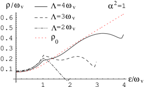
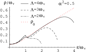
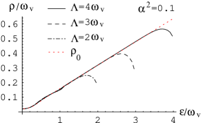
Figure 7: (color online) The full LDOS $\rho=\rho_{0}+\rho_{1}$ at the vortex center as a function of energy and quasiparticle cut-off $\Lambda$. The dotted red curve is $\rho_{0}(\epsilon)$, which excludes the resonant scattering and does not depend on any finite cut-off.

III.4 Influence of the Magnus force on the LDOS

When a vortex moves with respect to the superfluid, it experiences the Magus force. This force has the same effect on the vortex as magnetic field on a moving charged particle, so that it can be implemented through an effective gauge field $\boldsymbol{\mathcal{A}}$ in the vortex Hamiltonian:

$$H_{\textrm{v}}=\frac{(\boldsymbol{p}_{\textrm{v}}-\boldsymbol{\mathcal{A}})^{2}}{2m_{\textrm{v}}}+\frac{1}{2}m_{\textrm{v}}\omega_{\textrm{v}}^{2}\boldsymbol{r}_{\textrm{v}}^{2}\ ,$$ (51)

where ($\hbar=1$), for a Galilean-invariant superfluid,

$$\boldsymbol{\nabla}\times\boldsymbol{\mathcal{A}}=2\pi\rho_{\textrm{s}}\hat{\boldsymbol{z}}\ ,$$ (52)

and $\rho_{\textrm{s}}$ is the superfluid density (density of Cooper pairs). On a lattice, recent work CompOrd1 has argued that the rhs has to be replaced by difference between the density of Cooper pairs in the superfluid and half the density of electrons in a proximate solid. The presence of the Magnus force defines a corresponding cyclotron frequency:

$$\omega_{\textrm{m}}=\frac{2\pi\rho_{\textrm{s}}}{m_{\textrm{v}}}\ .$$ (53)

We assume that the vortex trap is isotropic, defining a single trap harmonic frequency $\omega_{\textrm{v}}$. Hence, both the trap and the Magnus force support circular classical trajectories of the vortex, making it easy to diagonalize the Hamiltonian  (51):

$$H_{\textrm{v}}=\omega_{0}+\omega_{+}^{\phantom{\dagger}}a_{+}^{\dagger}a_{+}^{\phantom{\dagger}}+\omega_{-}^{\phantom{\dagger}}a_{-}^{\dagger}a_{-}^{\phantom{\dagger}}\ ,$$ (54)

with

$$\omega_{0} = \sqrt{\omega_{\textrm{v}}^{2}+\left(\frac{\omega_{\textrm{m}}}{2}\right)^{2}}$$ (55)

$$\omega_{-} = \omega_{0}-\frac{\omega_{\textrm{m}}}{2}$$

$$\omega_{+} = \omega_{0}+\frac{\omega_{\textrm{m}}}{2}\ ,$$

and

$$a_{-} = \left(\frac{m_{\textrm{v}}\omega_{0}}{2}\right)^{\frac{1}{2}}\left(\frac{x_{\textrm{v}}+iy_{\textrm{v}}}{\sqrt{2}}+\frac{i}{m_{\textrm{v}}\omega_{0}}\frac{p_{x\textrm{v}}+ip_{y\textrm{v}}}{\sqrt{2}}\right)$$ (56)

$$a_{+} = \left(\frac{m_{\textrm{v}}\omega_{0}}{2}\right)^{\frac{1}{2}}\left(\frac{x_{\textrm{v}}-iy_{\textrm{v}}}{\sqrt{2}}+\frac{i}{m_{\textrm{v}}\omega_{0}}\frac{p_{x\textrm{v}}-ip_{y\textrm{v}}}{\sqrt{2}}\right)\ .$$

The full Hamiltonian includes coupling between the vortex and quasiparticles:

$$H=H_{\textrm{v}}+\sum_{\textrm{nodes}}\int\textrm{d}^{2}r\Psi^{\dagger}(\boldsymbol{r})H_{BdG}(\boldsymbol{r})\Psi^{\phantom{\dagger}}(\boldsymbol{r})\ ,$$ (57)

and we can proceed solving it just like before.

The Magnus force introduces only a few small changes in the LDOS obtained so far. First, the zero-point quantum motion of the vortex is now controlled by the frequency $\omega_{0}$, instead of $\omega_{\textrm{v}}$, which can be seen from  (56). The vortex ground-state wavefunction is still isotropic, but extends in space to distances $\sim(m_{\textrm{v}}\omega_{0})^{-1/2}$ from the trap center. Second, there are two small parameters, $\alpha_{+}=\sqrt{m_{\textrm{v}}\omega_{0}}/\omega_{+}$ and $\alpha_{-}=\sqrt{m_{\textrm{v}}\omega_{0}}/\omega_{-}$ that shape the perturbation theory. The frequencies $\omega_{+}$ and $\omega_{-}$ are important for the resonant scattering of quasiparticles from the vortex, and in principle, discontinuities in the LDOS can occur at these frequencies. The Magnus force lifts the degeneracy of vortex eigenmodes in an isotropic trap, so that the lowest excited states correspond to left and right handed circular motion of the vortex, with different energies.

In the Fig. 8 we compare the quasiparticle LDOS for several values of the Magnus cyclotron frequency $\omega_{\textrm{m}}$. In general, no qualitative changes arise when $\omega_{\textrm{m}}$ is finite, provided that it does not become too large ($\omega_{\textrm{m}}\sim 2\omega_{\textrm{v}}\Leftrightarrow\alpha_{-}\to 0$ would invalidate the perturbation theory). As $\omega_{\textrm{m}}$ grows, the sub-gap peak shifts toward smaller energies. Somewhat surprisingly the sharp features, such as the LDOS discontinuities, seem to become smoother as $\omega_{\textrm{m}}$ grows, although they do not completely vanish. In general, there is only one discontinuity at $\epsilon=\omega_{-}$.

Figure 8: The full LDOS at the vortex center as a function of energy, for different values of the Magnus cyclotron frequency $\omega_{\textrm{m}}$ (Eq. 53). The plots are offset vertically for clarity.

IV Discussion and conclusions

We have explored how the quantum motion of vortices affects quasiparticle spectra in clean $d$-wave superconductors at zero temperature. Keeping only the statistical interaction between vortices and quasiparticles in a continuum Bogoliubov-de Gennes model, we have found that quantum oscillations of a vortex could be responsible for observation of the “core states” in the STM experiments on cuprates. The emerging physical picture is that there are no bound states in the vortex core of an ideal $d$-wave superconductor, but quasiparticles can instead experience resonant scattering from a vortex. Vortices are localized either by their neighbors in a vortex lattice, or by pinning impurities, and execute zero-point quantum oscillations in their harmonic traps. When a quasiparticle scatters from a vortex, it can excite a virtual higher-energy state of vortex oscillations, and effectively form a short-lived metastable bound state with the vortex. This leads to a peak of the local density of states at the appropriate resonant energy in the vicinity of the vortex core. The peak lies inside the superconducting gap because the vortex zero-point motion extends over length-scales that are significantly larger than the coherence length.

Our numerically calculated LDOS has many similarities with experimental observations at energies smaller than the superconducting gap. The low energy scans of LDOS at various distances from the vortex core look qualitatively the same as the experimental measurements. We do not obtain a zero-energy peak that was originally predicted by meanfield BCS calculations Wang95 , and we find a small sub-gap peak that gradually vanishes with growing distance from the vortex core. We also find other features in the LDOS energy scans, such as discontinuities and secondary peaks and dips, but these may be blurred and too small to observe in realistic circumstances. According to our model, energy of the sub-gap peak turns out to be an increasing, but not a linear function of the superconducting gap. Experimental data appear to be consistent with the linear dependence, but due to large error margins in the measurements, and many simplifications built in our model, we believe that this detail cannot rule out the great importance of vortex quantum motion for quasiparticle spectra in $d$-wave superconductors.

The ability to reach a comprehensive physical picture of the sub-gap quasiparticle spectra comes with a price: our model contains many simplifications of realistic circumstances. Most approximations are controlled in the sense that there is a limit in which they become accurate. Away from that limit there will be quantitative modifications of the results due to other effects, such as thermal fluctuations, decoherence, and possible competing orders inside the vortex cores. We have also ignored anisotropies of $d$-wave superconductors. Perhaps the least justified simplification is inclusion of only the statistical interactions between vortices and quasiparticles. The missing Doppler shift presents an effective potential to quasiparticles near the vortex core, and may enhance the resonant scattering. We do not expect that it could qualitatively change the results, but its quantitative contribution need not be small.

We also reiterate here the original motivation for considering the vortex zero-point motion model. This arose from its consequences in the spatial dependence of the LDOS: it was argued CompOrd1 ; VorMass that the Aharanov-Bohm phases acquired by vortices from the background density of electrons lead naturally to periodic modulations in the LDOS. This was proposed as an explanation for the modulations observed in STM experiments hoffman ; fischer . Here we have shown that the same model can also help account for some crucial aspects of the energy dependence of the LDOS. Further, as argued in Ref. VorMass, , there is also a quantitative consistency between the energy scales deduced from the spatial and energy dependencies. From the extent of the spatial modulations,hoffman and an estimate of the trapping potential on a vortex, we were able to obtain an estimate of the vortex oscillation frequency.VorMass This number is consistent with the observed positionaprile ; pan ; hoffman of the sub-gap peaks in the energy dependence of the LDOS.

Future experiments may provide more ways to detect consequences of vortex quantum motion in $d$-wave superconductors. Neutron or light scattering measurements could provide a direct observation of the vortex oscillations. The spatial extent of the LDOS modulations provides means for measuring one important energy scale, $\sqrt{\hbar\omega_{\textrm{v}}m_{\textrm{v}}v_{\textrm{f}}^{2}}$, where $\omega_{\textrm{v}}$ is the harmonic frequency of a localized vortex. Our present prediction is that the sub-gap peak in the quasiparticle LDOS occurs at the energy proportional to this scale. An increased sensitivity of STM measurements in the future could allow resolving the jumps in the LDOS at energies that reflect the discrete spectrum of the trapped quantum vortex. This would provide means for measuring another important energy scale, $\hbar\omega_{\textrm{v}}$. Combined knowledge of both energy scales reveals the vortex mass $m_{\textrm{v}}$ and the strength of the vortex trapping force (inter-vortex interactions), which in turn can be related to other parameters, such as the superconducting gap and magnetic field. Effects of the Magnus force reduce to quantitative modifications of these energy scales, as discussed in the Section III.4.

Appendix A Calculation of vertex operators

Here we derive general expressions for the “matrix elements”  (8), which play the role of vertex operators in the perturbation theory. The matrix elements are evaluated by substituting the wavefunctions of the linear harmonic oscillator into  (8), and have the same form as the Hamiltonian  (3) in which the vector operator $\boldsymbol{a}$ is substituted by the vector c-number:

$$\boldsymbol{a}_{(n_{1x},n_{1y}),(n_{2x},n_{2y})}(\boldsymbol{r})=\frac{m_{\textrm{v}}\omega_{\textrm{v}}}{2\pi}\frac{2^{-(n_{1x}+n_{1y}+n_{2x}+n_{2y})/2}}{\sqrt{n_{1x}!n_{2x}!n_{1y}!n_{2y}!}}$$

$$~{}~{}~{}\times\int\textrm{d}^{2}r_{\textrm{v}}\frac{\hat{\boldsymbol{z}}\times(\boldsymbol{r}-\boldsymbol{r}_{\textrm{v}})}{2|\boldsymbol{r}-\boldsymbol{r}_{\textrm{v}}|^{2}}e^{-m_{\textrm{v}}\omega_{\textrm{v}}r_{\textrm{v}}^{2}}$$ (58)

$$~{}~{}~{}\times H_{n_{1x}}(x_{\textrm{v}}\sqrt{m_{\textrm{v}}\omega_{\textrm{v}}})H_{n_{1y}}(y_{\textrm{v}}\sqrt{m_{\textrm{v}}\omega_{\textrm{v}}})$$

$$~{}~{}~{}\times H_{n_{2x}}(x_{\textrm{v}}\sqrt{m_{\textrm{v}}\omega_{\textrm{v}}})H_{n_{2y}}(y_{\textrm{v}}\sqrt{m_{\textrm{v}}\omega_{\textrm{v}}})\ .$$

$H_{n}(x)$ are Hermite polynomials of order $n$. One way to analytically calculate these integrals is to use the following formula:

$$\frac{\hat{\boldsymbol{z}}\times(\boldsymbol{r}-\boldsymbol{r}_{\textrm{v}})}{2|\boldsymbol{r}-\boldsymbol{r}_{\textrm{v}}|^{2}}=\frac{1}{2}\hat{\boldsymbol{z}}\times\left(\boldsymbol{\nabla}\log|\boldsymbol{r}-\boldsymbol{r}_{\textrm{v}}|\right)\ ,$$ (59)

and expand:

$$\log|\boldsymbol{r}-\boldsymbol{r}_{\textrm{v}}|=\log|z-z_{\textrm{v}}|=\log\left|z_{>}\left(1-\frac{z_{<}}{z_{>}}\right)\right|$$

$$~{}~{}~{}~{}~{}=\log|z_{>}|+\frac{1}{2}\log\left(1-\frac{z_{<}}{z_{>}}\right)+\frac{1}{2}\log\left(1-\frac{z_{<}^{*}}{z_{>}^{*}}\right)$$

$$~{}~{}~{}~{}~{}=\log|z_{>}|-\textrm{Re}\sum_{n=1}^{\infty}\frac{1}{n}\left(\frac{z_{<}}{z_{>}}\right)^{n}\ .$$ (60)

Coordinates have been represented by complex numbers $z$ and $z_{\textrm{v}}$; $z_{>}$ and $z_{<}$ are the greater and lesser by modulus of $z$ and $z_{\textrm{v}}$ respectively. The effective gauge-field  (A) is:

$$\boldsymbol{a}_{(n_{1x},n_{1y}),(n_{2x},n_{2y})}(\boldsymbol{r})~{}\propto~{}$$ (61)

$$~{}~{}~{}\propto\hat{\boldsymbol{z}}\times\boldsymbol{\nabla}\int\textrm{d}^{2}z_{\textrm{v}}\left[\log|z_{>}|-\textrm{Re}\sum_{n=1}^{\infty}\frac{1}{n}\left(\frac{z_{<}}{z_{>}}\right)^{n}\right]\times$$

$$~{}~{}~{}~{}~{}~{}~{}e^{-m_{\textrm{v}}\omega_{\textrm{v}}|z_{\textrm{v}}|^{2}}H_{n_{1x}}H_{n_{1y}}H_{n_{2x}}H_{n_{2y}}\ .$$

The Hermite polynomials are easily written in terms of $z_{\textrm{v}}$ and $z_{\textrm{v}}^{*}$ at low orders $n$. For any particular set of $(n_{1x},n_{1y},n_{2x},n_{2y})$ only one term in the expansion above gives a non-zero contribution upon integration of the phase of $z_{\textrm{v}}$. For example, when $n_{1x}=n_{1y}=n_{2x}=n_{2y}=0$ all Hermite polynomials are equal to unity, and the only term that does not depend on phase is the logarithm:

$$\boldsymbol{a}_{(0,0),(0,0)} = m_{\textrm{v}}\omega_{\textrm{v}}\hat{\boldsymbol{z}}\times\boldsymbol{\nabla}\Biggl{[}\int\limits_{0}^{|z|}\textrm{d}|z_{\textrm{v}}|e^{-m_{\textrm{v}}\omega_{\textrm{v}}|z_{\textrm{v}}|^{2}}\log(|z|)+$$

$$\int\limits_{|z|}^{\infty}\textrm{d}|z_{\textrm{v}}|e^{-m_{\textrm{v}}\omega_{\textrm{v}}|z_{\textrm{v}}|^{2}}\log(|z_{\textrm{v}}|)\Biggr{]}$$

$$= m_{\textrm{v}}\omega_{\textrm{v}}\hat{\boldsymbol{z}}\times\hat{\boldsymbol{r}}\frac{\partial}{\partial r}\log(r)\int_{0}^{r}\textrm{d}r_{\textrm{v}}r_{\textrm{v}}e^{-m_{\textrm{v}}\omega_{\textrm{v}}r_{\textrm{v}}^{2}}$$

$$= \hat{\boldsymbol{z}}\times\frac{\boldsymbol{r}}{r^{2}}\left(1-e^{-m_{\textrm{v}}\omega_{\textrm{v}}r^{2}}\right)\ .$$

This is the result written in  (4). A similar calculation produces the expression  (III.2).

Appendix B Calculation of the one-loop correction to the LDOS

Here we substitute  (37) and  (III.2) into  (III.3) and derive the lowest order correction to the LDOS. We systematically use the formula:

$$\frac{1}{\omega-\epsilon+i0^{+}}=\frac{\mathbb{P}}{\omega-\epsilon}-i\pi\delta(\omega-\epsilon)$$ (63)

to extract the imaginary part in  (III.3). After a few algebraic manipulations one obtains the following correction to the LDOS:

$$\rho_{1}(\epsilon,\boldsymbol{r})=\textrm{sign}(\epsilon)\sum_{l_{1},l_{2}}\sum_{l}\textrm{Tr}\Biggl{\{}$$ (64)

$$-\pi^{2}T_{l_{1},|\epsilon|}^{\phantom{\dagger}}(\boldsymbol{r})\left(\begin{array}[]{cc}\scriptstyle\Theta(\epsilon)&\scriptstyle 0\\ \scriptstyle 0&\scriptstyle-\Theta(-\epsilon)\end{array}\right)V^{\mu}_{l_{1},|\epsilon|;l,|\epsilon|-\omega_{\textrm{v}}}\left(\begin{array}[]{cc}\scriptstyle\Theta(\epsilon-\omega_{\textrm{v}})&\scriptstyle 0\\ \scriptstyle 0&\scriptstyle-\Theta(-\epsilon-\omega_{\textrm{v}})\end{array}\right)V^{\mu}_{l,|\epsilon|-\omega_{\textrm{v}};l_{2},|\epsilon|}\left(\begin{array}[]{cc}\scriptstyle\Theta(\epsilon)&\scriptstyle 0\\ \scriptstyle 0&\scriptstyle-\Theta(-\epsilon)\end{array}\right)T_{l_{2},|\epsilon|}^{\dagger}(\boldsymbol{r})$$ (71)

$$+\int\textrm{d}k_{1}\textrm{d}k_{2}T_{l_{1},k_{1}}^{\phantom{\dagger}}(\boldsymbol{r})\left(\begin{array}[]{cc}\scriptstyle\frac{\mathbb{P}}{\epsilon-k_{1}}&\scriptstyle 0\\ \scriptstyle 0&\scriptstyle\frac{\mathbb{P}}{\epsilon+k_{1}}\end{array}\right)V^{\mu}_{l_{1},k_{1};l,|\epsilon|-\omega_{\textrm{v}}}\left(\begin{array}[]{cc}\scriptstyle\Theta(\epsilon-\omega_{\textrm{v}})&\scriptstyle 0\\ \scriptstyle 0&\scriptstyle-\Theta(-\epsilon-\omega_{\textrm{v}})\end{array}\right)V^{\mu}_{l,|\epsilon|-\omega_{\textrm{v}};l_{2},k_{2}}\left(\begin{array}[]{cc}\scriptstyle\frac{\mathbb{P}}{\epsilon-k_{2}}&\scriptstyle 0\\ \scriptstyle 0&\scriptstyle\frac{\mathbb{P}}{\epsilon+k_{2}}\end{array}\right)T_{l_{2},k_{2}}^{\dagger}(\boldsymbol{r})$$ (78)

$$+\int\textrm{d}k_{2}\textrm{d}kT_{l_{1},|\epsilon|}^{\phantom{\dagger}}(\boldsymbol{r})\left(\begin{array}[]{cc}\scriptstyle\Theta(\epsilon)&\scriptstyle 0\\ \scriptstyle 0&\scriptstyle-\Theta(-\epsilon)\end{array}\right)V^{\mu}_{l_{1},|\epsilon|;l,k}\left(\begin{array}[]{cc}\scriptstyle\frac{\mathbb{P}}{\epsilon-k-\omega_{\textrm{v}}}&\scriptstyle 0\\ \scriptstyle 0&\scriptstyle\frac{\mathbb{P}}{\epsilon+k+\omega_{\textrm{v}}}\end{array}\right)V^{\mu}_{l,k;l_{2},k_{2}}\left(\begin{array}[]{cc}\scriptstyle\frac{\mathbb{P}}{\epsilon-k_{2}}&\scriptstyle 0\\ \scriptstyle 0&\scriptstyle\frac{\mathbb{P}}{\epsilon+k_{2}}\end{array}\right)T_{l_{2},k_{2}}^{\dagger}(\boldsymbol{r})$$ (85)

$$+\int\textrm{d}k\textrm{d}k_{1}T_{l_{1},k_{1}}^{\phantom{\dagger}}(\boldsymbol{r})\left(\begin{array}[]{cc}\scriptstyle\frac{\mathbb{P}}{\epsilon-k_{1}}&\scriptstyle 0\\ \scriptstyle 0&\scriptstyle\frac{\mathbb{P}}{\epsilon+k_{1}}\end{array}\right)V^{\mu}_{l_{1},k_{1};l,k}\left(\begin{array}[]{cc}\scriptstyle\frac{\mathbb{P}}{\epsilon-k-\omega_{\textrm{v}}}&\scriptstyle 0\\ \scriptstyle 0&\scriptstyle\frac{\mathbb{P}}{\epsilon+k+\omega_{\textrm{v}}}\end{array}\right)V^{\mu}_{l,k;l_{2},|\epsilon|}\left(\begin{array}[]{cc}\scriptstyle\Theta(\epsilon)&\scriptstyle 0\\ \scriptstyle 0&\scriptstyle-\Theta(-\epsilon)\end{array}\right)T_{l_{2},|\epsilon|}^{\dagger}(\boldsymbol{r})\Biggr{\}}\ .$$ (92)

This expression for $\rho_{1}$ is written assuming that the sample is infinite. In order to carry out numerical calculations it is necessary to impose a finite sample radius $R$ and thus quantize energy levels of the unperturbed Hamiltonian. The quantized energies take values $\epsilon_{n}=\pm k_{n}$, where $k_{n}R+\delta$ is the $n^{\textrm{th}}$ zero of the Bessel function ($\delta$ is a phase shift). In the region $k_{n}R\gg 1$, the energy levels are separated by $\pi/R$, and this allows a simple rule of thumb for conversion between the continuous and discrete computations. First, the infinite-sample wavefunctions need to be renormalized to unity on the finite sample. Up to a small error of the order $(k_{n}R)^{-1}$ this amounts to multiplying the wavefunction by $\sqrt{\pi/R}$. Second, all integrations over continuous radial wave-vectors $k$ in the expression  (64) must be replaced by summations over discrete $k_{n}$, with a measure factor of $\pi/R$. Finally, the principal part $\mathbb{P}/x$ is taken to deviate from $1/x$ in the interval of width $\pi/R$ from $x=0$, passing smoothly through zero at $x=0$.

As a result of energy discretization, the LDOS is strictly speaking defined only at discrete energy levels $\epsilon_{n}$. Such discretization is naturally lifted if there are additional fluctuations in the problem that broaden the energy levels beyond $\pi/R$ (for example, due to finite temperature or disorder). However, the level-broadening mechanisms are not important in the $R\to\infty$ limit, which is reached in numerics if the majority of states satisfy $k_{n}R\gg 1$ (that is, if the energy cut-off $\Lambda$ is large, $\Lambda R\gg 1$). The typical values that we used in numerics were $R=200$, $\Lambda=4$, $\omega_{\textrm{v}}=1$, and $-5\leq l\leq 5$.

Appendix C Microscopic theory for a $d$-wave superconductor

This appendix connects the results of the present paper to those of paper I. Here we will extend the numerical results of I to $d$-wave superconductors. However, because of the gradient expansion necessary in this method, we are unable to extend these results to very small vortex core sizes. Consequently, we will not find an elimination of the zero bias peak in the LDOS.

As discussed in I, we will use the gap operator given in Eq. (3) of I, with $\Delta({\bf r})=\Delta(r)e^{i\theta}$. In polar coordinates which are more convenient for our problem here this gap operator reads

$$\hat{\Delta}= \frac{e^{3i\theta}}{8k_{F}^{2}r^{2}}\left[(3\Delta-3r\Delta^{\prime}+r^{2}\Delta^{\prime\prime})+4(-2r\Delta+r^{2}\Delta^{\prime})\partial_{r}+4i(-3\Delta+r\Delta^{\prime})\partial_{\theta}+4\Delta(r^{2}\partial_{r}^{2}-\partial_{\theta}^{2}+2ir\partial_{r}\partial_{\theta})\right]$$

$$+ \frac{e^{-i\theta}}{8k_{F}^{2}r^{2}}\left[(-\Delta+r\Delta^{\prime}+r^{2}\Delta^{\prime\prime})+4r^{2}\Delta^{\prime}\partial_{r}+4i(\Delta-r\Delta^{\prime})\partial_{\theta}+4\Delta(r^{2}\partial_{r}^{2}-\partial_{\theta}^{2}-2ir\partial_{r}\partial_{\theta})\right]\;.$$ (93)

As a generalization of Eqs. (21) and (31) of I we write the quasi-particle wave functions as

$$\left(\begin{array}[]{c}u_{\ell}({\bf r})\\ v_{\ell}({\bf r})\end{array}\right)=\sum_{mj}\left(\begin{array}[]{c}c_{mj}^{(\ell)}\phi_{m,j}({\bf r})\\ d_{mj}^{(\ell)}\phi_{m,j}({\bf r})\end{array}\right)\;,$$ (94)

where the

$$\phi_{m,j}({\bf r})\equiv\phi_{m,j}(r,\theta)\equiv\exp[-im\theta]\phi_{mj}(r)/\sqrt{2\pi}$$ (95)

[which generalize Eq. (29) of I] now form a complete set of eigenfunctions to the kinetic energy operator and satisfy the normalization condition

$$\int_{0}^{2\pi}d\theta\int_{0}^{R_{0}}dr\,r\,\phi_{mj}^{\ast}(r,\theta)\,\phi_{m^{\prime}j^{\prime}}(r,\theta)=\delta_{mm^{\prime}}\delta_{jj^{\prime}}\;.$$ (96)

The Bogoliubov-de Gennes equations reduce to a matrix equation quite similar to Eq. (32) of I. The essential difference is that there is now an infinite hierarchy of coupled angular momentum channels and the matrices $T^{\pm}$ and $\Delta$ now have matrix elements

$$T_{mj;m^{\prime}j^{\prime}}^{\pm}= \,\mp\frac{1}{2m_{e}}\left(\frac{\alpha_{m,j}^{2}}{R_{0}^{2}}-k_{F}^{2}\right)\delta_{m,m^{\prime}}\delta_{jj^{\prime}}\;,$$ (97)

$$\Delta_{mj;m^{\prime}j^{\prime}}= \int_{0}^{2\pi}d\theta\int_{0}^{R_{0}}dr\,r\,\phi_{m,j}^{\ast}(r,\theta)\hat{\Delta}\,\phi_{m^{\prime},j^{\prime}}(r,\theta)\;.$$ (98)

Using the gap operator given in Eq. (93) we can explicitly evaluate $\Delta_{mj;m^{\prime}j^{\prime}}$ and obtain

$$\Delta_{mj;m^{\prime}j^{\prime}}=\delta_{m^{\prime},m+3} \int_{0}^{R_{0}}dr\,\frac{\phi_{m,j}(r)}{8k_{F}^{2}r}\big{\{}\left[(-4(\alpha_{m+3,j^{\prime}}r/R_{0})^{2}+3)\Delta-3r\Delta^{\prime}+r^{2}\Delta^{\prime\prime}\right]\phi_{m+3,j^{\prime}}(r)\big{.}$$

. $$\qquad\qquad\qquad\qquad\quad{}+4\left[(2m+3)\Delta+r\Delta^{\prime}\right]\phi_{m+3,j^{\prime}}^{-}(r)\big{\}}$$

$${}+\delta_{m^{\prime},m-1} \int_{0}^{R_{0}}dr\,\frac{\phi_{m,j}(r)}{8k_{F}^{2}r}\big{\{}\left[(-4(\alpha_{m-1,j^{\prime}}r/R_{0})^{2}-1)\Delta+r\Delta^{\prime}+r^{2}\Delta^{\prime\prime}\right]\phi_{m-1,j^{\prime}}(r)\big{.}$$

. $$\qquad\qquad\qquad\qquad\quad{}+4\left[(2m-1)\Delta-r\Delta^{\prime}\right]\phi_{m-1,j^{\prime}}^{+}(r)\big{\}}\;.$$ (99)

The functions

$$\phi_{m,j}^{\pm}\equiv\frac{\sqrt{2}\,\alpha_{m,j}r}{R_{0}^{2}|J_{m+1}(\alpha_{m,j})|}J_{m\pm 1}(\alpha_{m,j}r/R_{0})$$ (100)

are modifications of the normalized Bessel functions $\phi_{m,j}(r)$ defined in Eq. (29) of I which arise when taking derivatives of $\phi_{m,j}(r)$. According to Eq. (99) $m^{\prime}$ has to equal $m-1$ or $m+3$ for a matrix element not to vanish. The reason for this is that while the vortex in the order parameter mediates a change in $m$ (minus angular momentum) by $1$ when scattering the hole-like component of the quasi-particle into an electron-like component, due to the $d$-wave symmetry of the gap operator we have an additional change by $\pm 2$. As a consequence of this, the eigenvalue problem breaks up into four apparently independent eigenvalue problems which we all truncate at large angular momentum $m_{\text{max}}$.

Let us say that the eigenvector $\Psi_{\ell}$ lies in the sector $s(\ell)=0,1,2$, or $3$ if $\Psi_{\ell}$ contains only components $c_{4\nu+s}$ and $d_{4\nu+s-1}$ with $\nu$ an integer. It is possible to write the eigenvalue problem for each of these four sectors in terms of a real and symmetric band-diagonal matrix. For concreteness, let us consider the sector $s=0$ with $m_{\text{max}}=5$ (which, of course, for practical calculations should be chosen much larger). We then have

$$\left(\begin{array}[]{llllll}T_{-5}^{+}&\Delta_{-4;-5}^{T}&&&&0\\ \Delta_{-4;-5}&T_{-4}^{-}&\Delta_{-4;-1}&&&\\ &\Delta_{-4;-1}^{T}&T_{-1}^{+}&\Delta_{0;-1}^{T}&&\\ &&\Delta_{0;-1}&T_{0}^{-}&\Delta_{0;3}&\\ &&&\Delta_{0;3}^{T}&T_{3}^{+}&\Delta_{4;3}^{T}\\ 0&&&&\Delta_{4;3}&T_{4}^{-}\\ \end{array}\right)\Psi_{\ell}^{(s)}=\epsilon_{\ell}^{(s)}\,\Psi_{\ell}^{(s)}\;.$$ (101)

Here, $T_{m}^{\pm}$ and $\Delta_{m;m^{\prime}}$ are themselves $N_{0}\times N_{0}$ matrices whose matrix elements are given above. We can now relate each eigenstate in sector $1$ to one in sector $0$ and each eigenstate in sector $3$ to one in sector $2$ by making use of the property that if $[u_{\ell}({\bf r}),v_{\ell}({\bf r})]^{T}$ is an eigenstate of $\mathcal{H}_{\text{BdG}}^{0}$ with eigenvalue $\epsilon_{\ell}$, then $[-v_{\ell}^{\ast}({\bf r}),u_{\ell}^{\ast}({\bf r})]^{T}$ is an eigenstate of $\mathcal{H}_{\text{BdG}}^{0}$ with eigenvalue $-\epsilon_{\ell}$. This property implies the symmetry

$$\Delta_{mj;m^{\prime}j^{\prime}}=-\Delta_{-m^{\prime},j^{\prime};-m,j}\;,$$ (102)

which we have checked explicitly. In terms of the eigenvectors $\Psi=(c_{4\nu+s},d_{4\nu+s-1})$ we find that if $\Psi$ is an eigenvector in sector $s$ with eigenvalue $\epsilon$, then $\tilde{\Psi}=(\tilde{c}_{4\nu+(1-s)},\tilde{d}_{4\nu+(1-s)-1})$ with $\tilde{c}_{m,j}\equiv d_{-m,j}$ and $\tilde{d}_{m,j}\equiv c_{-m,j}$ is an eigenvector with eigenvalue $-\epsilon$ in sector $1-s\,(\text{mod}\,4)$. It is therefore sufficient to only consider the sectors $0$ and $2$ and make use of this property to obtain all eigenstates.

An interesting property of having no mixing between the four sectors is that the quasi particle amplitudes $u_{\ell}^{(s)}({\bf r})$ and $v_{\ell}^{(s)}({\bf r})$ can be written as

$$u_{\ell}^{(s)}({\bf r})= \frac{e^{-is\theta}}{\sqrt{2\pi}}\sum_{\nu,j}c_{4\nu+s,j}^{(\ell)}e^{-4i\nu\theta}\phi_{4\nu+s,j}(r)\;,$$ (103)

$$v_{\ell}^{(s)}({\bf r})= \frac{e^{-i(s-1)\theta}}{\sqrt{2\pi}}\sum_{\nu,j}d_{4\nu+s-1,j}^{(\ell)}e^{-4i\nu\theta}\phi_{4\nu+s-1,j}(r)\;.$$ (104)

Physically measurable quantities like the local DOS which only involve $|u_{\ell}^{(s)}({\bf r})|^{2}$ (and $|v_{\ell}^{(s)}({\bf r})|^{2}$) are therefore invariant under all symmetry operations expected for a $d_{x^{2}-y^{2}}$-wave order parameter, i.e. rotations by $90^{\circ}$ as well as reflections along the nodal or anti-nodal directions. Before considering the effect of the zero-point fluctuations of the vortex on the local DOS let us first have a look at the case of a static vortex which was already studied in Refs. Wang95, ; Franz98, . One advantage of using the gap operator given in Eq. (93) is that most of its matrix elements $\Delta_{mj;m^{\prime}j^{\prime}}$ cancel. We can therefore calculate the local DOS for reasonably large system sizes with moderate computational effort.

In Fig. 9 we show results for the angular average of the tunneling conductance $G({\bf r},\omega)$ for various values of $r$ calculated for a system with radius $k_{F}R=120$ and a cutoff $m_{\text{max}}=60$ for the angular momentum channels. Directly at the vortex center there is a peak in the local DOS near the Fermi level which is due to a continuum of unlocalized states whose envelopes take there maximum near the vortex center but which have tails leaking out in the nodal directions. These results are consistent with those found in Refs. Wang95, ; Franz98, . As we move away from the vortex center the peak in the local DOS gradually vanishes and the tunneling conductance assumes the familiar features of a $d$-wave bulk spectrum (at finite temperature).

To calculate the transition matrix elements $M_{\ell,\ell^{\prime}}^{\alpha}$ which were defined in Eq. (15) of I we will use the Hellmann-Feynman theorem which in the present case of a $d$-wave gap operator reads

$$M_{\ell,\ell^{\prime}}^{+} =(\epsilon_{\ell^{\prime}}-\epsilon_{\ell})U_{\ell;\ell^{\prime}}^{+}-\frac{R_{0}}{2m_{e}}\int_{0}^{2\pi}d\theta\,\partial_{r}\Psi_{\ell}^{\dagger}\sigma_{3}\partial_{\bar{z}}\Psi_{\ell^{\prime}}\Big{|}_{r=R_{0}}$$

$$\quad{}+\frac{\Delta(R_{0})R_{0}}{2k_{F}^{2}}\int_{0}^{2\pi}d\theta\,(e^{3i\theta}+e^{-i\theta})\partial_{r}u_{\ell}^{\ast}\partial_{\bar{z}}v_{\ell^{\prime}}\Big{|}_{r=R_{0}}$$

$$\quad{}+\frac{\Delta(R_{0})R_{0}}{2k_{F}^{2}}\int_{0}^{2\pi}d\theta\,(e^{-3i\theta}+e^{i\theta})\partial_{r}v_{\ell}^{\ast}\partial_{\bar{z}}u_{\ell^{\prime}}\Big{|}_{r=R_{0}}\;.$$ (105)

The first two terms are as in the $s$-wave case but since our $d$-wave operator involves two derivatives, partial integration now also leads to a boundary term involving the bulk gap. In the $s$-wave case angular momentum was a good quantum number and for a transition matrix element not to vanish we had the selection rule that the angular momenta of the two wave functions had to differ by one. As already emphasized above, in the $d$-wave case angular momentum is not a good quantum number. Instead, each eigenstate belongs to one of four sectors which only contains certain angular momentum channels. As a result of this we find that the transition matrix elements $M_{\ell,\ell^{\prime}}^{+}=M_{\ell^{\prime},\ell}^{-}$ are only non-zero if $s^{\prime}(\ell^{\prime})=s(\ell)+1\,(\text{mod}\,4)$. In this case we can again express all wave functions in terms of their Fourier-Bessel components and obtain

$$M_{\ell,\ell^{\prime}}^{+}=\, \frac{1}{2}\sum_{m=4\nu+s}\sum_{jj^{\prime}}c_{mj}^{(\ell)}\left[(\epsilon_{\ell^{\prime}}-\epsilon_{\ell})\mathcal{K}_{jj^{\prime}}^{(m)}-\mathcal{L}_{jj^{\prime}}^{(m)}\right]c_{m+1,j^{\prime}}^{(\ell^{\prime})}+\frac{1}{2}\sum_{m=4\nu+s-1}\sum_{jj^{\prime}}d_{mj}^{(\ell)}\left[(\epsilon_{\ell^{\prime}}-\epsilon_{\ell})\mathcal{K}_{jj^{\prime}}^{(m)}+\mathcal{L}_{jj^{\prime}}^{(m)}\right]d_{m+1,j^{\prime}}^{(\ell^{\prime})}$$

$$+ \frac{\Delta(R_{0})}{2k_{F}^{2}R_{0}^{3}}\sum_{m=4\nu+s}\sum_{jj^{\prime}}\left\{c_{mj}^{(\ell)}(-1)^{j-j^{\prime}}\alpha_{mj}\alpha_{mj^{\prime}}d_{mj^{\prime}}^{(\ell^{\prime})}+c_{mj}^{(\ell)}(-1)^{j-j^{\prime}}\eta_{-1}(m)\,\eta_{-3}(m)\,\alpha_{mj}\alpha_{m+4,j^{\prime}}d_{m+4,j^{\prime}}^{(\ell^{\prime})}\right\}$$

$$+ \frac{\Delta(R_{0})}{2k_{F}^{2}R_{0}^{3}}\sum_{m=4\nu+s-1}\sum_{jj^{\prime}}\left\{d_{mj}^{(\ell)}(-1)^{j-j^{\prime}}\eta_{1}(m)\alpha_{mj}\alpha_{m-2,j^{\prime}}c_{m-2,j^{\prime}}^{(\ell^{\prime})}+d_{mj}^{(\ell)}(-1)^{j-j^{\prime}}\eta_{-1}(m)\,\alpha_{mj}\alpha_{m+2,j^{\prime}}c_{m+2,j^{\prime}}^{(\ell^{\prime})}\right\}\;,$$ (106)

where the matrix elements $\mathcal{K}_{jj^{\prime}}^{(m)}$ and $\mathcal{L}_{jj^{\prime}}^{(m)}$ were already defined in Eqs. (40) and (41) of I and $\eta_{n}(m)\equiv 1-2\delta_{n,m}$ leads to an extra minus sign if $m=n$.

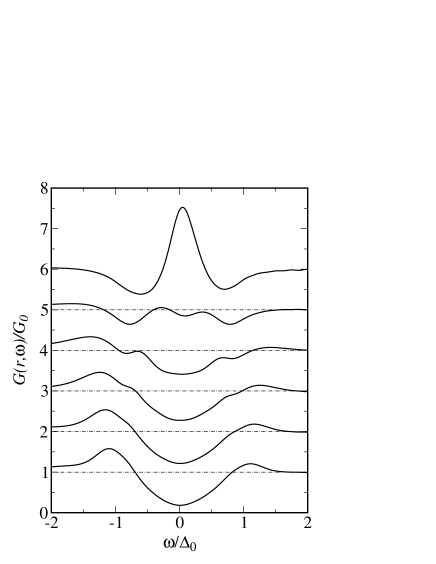
Figure 9: Angular average of the tunneling conductance $G=\partial I/\partial V$ for a superconductor with $d_{x^{2}-y^{2}}$ wave symmetry and a static vortex at the origin as a function of $\omega$. We have chosen $k_{F}\xi=2.5$ and $T=0.02\,E_{F}$. The upper curve is for $r=0$ and the curves below are for $k_{F}r=4,8,\dots,20$.

Figure 10: Angular average of the tunneling conductance $G=\partial I/\partial V$ for a superconductor with $d_{x^{2}-y^{2}}$ wave symmetry and a vortex with vortex mass $m_{v}=m_{e}$ as a function of $\omega$. We have chosen $k_{F}\xi=2.5$ and $T=0.02\,E_{F}$. The upper curve is for $r=0$ and the curves below are for $k_{F}r=4,8,\dots,20$.

The tunneling conductance calculated for the parameters used above but with a vortex mass equal to the mass of an electron is shown in Fig. 10. As seen in experiments, the central peak in the vortex center is suppressed and weight is shifted to both sides away from the Fermi level. Although the mechanism for redistributing spectral weight is the same as in the $s$-wave case no satellite peaks are visible in the $d$-wave case. The redistribution of spectral weight is further illustrated in Fig. 11 where we compare our results for a static vortex with those for a moving vortex.

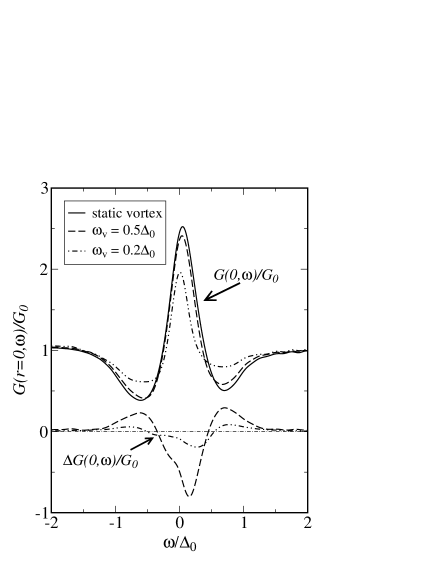
Figure 11: Comparison of the tunneling conductance $G=\partial I/\partial V$ for a superconductor with $d_{x^{2}-y^{2}}$ wave symmetry in the presence of a static or moving vortex. The upper curve shows the tunneling conductance at the vortex center for a static vortex (with $k_{F}\xi=2.5$ and $T=0.02\,E_{F}$). As we allow for a finite vortex mass and vortex frequency the cental peak decreases and weight is shifted away from the Fermi level. This is shown in the two curves below for which we have chosen $m_{v}=m_{e}$ and $\omega_{v}=0.2\,\Delta_{0}$ or $\omega_{v}=0.5\,\Delta_{0}$ respectively. Finally, the two curves at the bottom of the figure represent the difference between the results for the case of a moving vortex and that of a static vortex.

As can be seen in that figure, choosing a smaller vortex frequency $\omega_{v}$ leads to a much stronger redistribution of spectral weight. This is a direct consequence of Eqs. (16) and (17) of I. Also, although there are no sub-gap peaks visible in the tunneling conductance, the curves for the difference between the tunneling conductance for a moving and that for a static vortex show peaks at an energy significantly smaller than the gap energy, which according to Eq. (16) of I should be of the order of the vortex frequency.

Although our theory explains the redistribution of spectral weight from the zero bias level towards higher energies, it cannot explain the exact line shape as observed in experiment. First of all, the system sizes studied are much smaller than in the $s$-wave case, leading to a poorer spectral resolution. Angular momentum is not a good quantum number and a large number of angular momentum channels is needed to obtain convergence. This is shown in Fig. 12 where we compare results for the tunneling conductance at the vortex center, calculated with different cutoffs $m_{\text{m}ax}$ implemented.

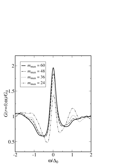
Figure 12: Comparison of results for the tunneling conductance $G=\partial I/\partial V$ at the vortex center of a superconductor with $d_{x^{2}-y^{2}}$ wave symmetry in the presence of a moving vortex. As in the previous figures, we have considered a system with radius $k_{F}R_{0}=120$, $k_{F}\xi=2.5$ and $T=0.02\,E_{F}$. The only difference is that we have used different cutoffs ($m_{\text{max}}=24,\,36,\,48$, and $60$) for the angular momentum channels.

As can be seen in that figure, we have not even achieved convergence for $m_{\text{max}}=60$, the value used in all the previous figures. However, it seems that we are not too far away from the $m_{\text{m}ax}\to\infty$ limit. (It should also be noted that an unphysical peak at $\approx+\Delta_{0}$ as seen for $m_{\text{m}ax}=24$ or $36$ is basically absent for $m_{\text{m}ax}=60$.)

The above scenario is quite different from the case of a static vortex where a cutoff of $m_{\text{m}ax}=24$ suffices to obtain convergence. We therefore conclude that it must be the transition matrix elements $M_{\ell,\ell^{\prime}}^{\pm}$ which are very sensitive to the boundary conditions imposed by the cutoff $m_{\text{m}ax}$. Another restriction on the applicability of our theory is our expansion of the gap operator $\hat{\Delta}({\bf r}-{\bf R}(\tau))$ to leading order in ${\bf R}(\tau)$. Since the quantum zero-point motion of the vortex basically extends roughly over a distance of $1/\sqrt{m_{v}\omega_{v}}$ from the vortex center this approximation is only expected to be reasonable as long as $\xi\gg 1/\sqrt{m_{v}\omega_{v}}$. We are therefore not able to study systems with very small coherence lengths.

References

- (1) L. Bartosch and S. Sachdev, cond-mat/0604105 (2006).
- (2) L. Balents, L. Bartosch, A. Burkov, S. Sachdev, and K. Sengupta, Phys. Rev. B 71, 144508 (2005).
- (3) L. Bartosch, L. Balents, and S. Sachdev, Ann. Phys. (New York) 321, 1528 (2006).
- (4) J. E. Hoffman, E. W. Hudson, K. M. Lang, V. Madhavan, S. H. Pan, H. Eisaki, S. Uchida, and J. C. Davis, Science 295, 466 (2002).
- (5) G. Levy, M. Kugler, A. A. Manuel, Ø. Fischer, and M. Li, Phys. Rev. Lett. 95, 257005 (2005).
- (6) Y. Wang and A. H. MacDonald, Phys. Rev. B 52, R 3876 (1995).
- (7) M. Ichioka, N. Hayashi, N. Enomoto, and K. Machida, Phys. Rev. B 53, 15316 (1996).
- (8) M. Franz and Z. Tešanović, Phys. Rev. Lett. 80, 4763 (1998).
- (9) J.-X. Zhu and C. S. Ting, Phys. Rev. Lett. 87, 147002 (2001); H.-Y. Chen and C. S. Ting, Phys. Rev. B 71, 220510(R) (2005).
- (10) A. Ghosal, C. Kallin, and A. J. Berlinsky Phys. Rev. B 66, 214502 (2002); D. Knapp, C. Kallin, A. Ghosal, and S. Mansour Phys. Rev. B 71, 064504 (2005).
- (11) H. Tsuchiura, M. Ogata, Y. Tanaka, and S. Kashiwaya, Phys. Rev. B 68, 012509 (2003).
- (12) I. Maggio-Aprile, Ch. Renner, A. Erb, E. Walker and Ø. Fischer, Phys. Rev. Lett. 75, 2754 (1995).
- (13) S. H. Pan, E. W. Hudson, A. K. Gupta, K.-W. Ng, H. Eisaki, S. Uchida, and J. C. Davis, Phys. Rev. Lett. 85, 1536 (2000).
- (14) B. W. Hoogenboom, K. Kadowaki, B. Revaz, M. Li, Ch. Renner, and Ø. Fischer, Phys. Rev. Lett. 87, 267001 (2001).
- (15) V. J. Emery and S. A. Kivelson, Nature 374, 434 (1995).
- (16) O. Vafek, A. Melikyan, M. Franz, and Z. Tešanović, Phys. Rev. B 63, 134509 (2001).
- (17) A. Melikyan and Z. Tešanović, cond-mat/0605314.
- (18) P. Nikolić and S. Sachdev, Phys. Rev. B 73, 134511 (2006).