Universal fluctuation of the average height in the early-time regime of the one-dimensional Kardar-Parisi-Zhang-type growth

Abstract

The statistics of the average height fluctuation of the one-dimensional Kardar-Parisi-Zhang(KPZ)-type surface is investigated. Guided by the idea of local stationarity, we derive the scaling form of the characteristic function in the early-time regime, $t\ll N^{3/2}$ with $t$ time and $N$ the system size, from the known characteristic function in the stationary state ($t\gg N^{3/2}$) of the single-step model derivable from a Bethe Ansatz solution, and thereby find the scaling properties of the cumulants and the large deviation function in the early-time regime. These results, combined with the scaling analysis of the KPZ equation, imply the existence of the universal scaling functions for the cumulants and an universal large deviation function. The analytic predictions are supported by the simulation results for two different models.

Keywords: Kinetic growth processes (Theory), Fluctuations (theory), Integrable spin chains (vertex models)

1 Introduction

The Kardar-Parisi-Zhang (KPZ) equation [1] is a nonlinear differential equation with noise representing in the simplest way the roughening phenomena of growing surfaces. The roughness is measured by the spatial fluctuation of the surface profile, and an initially flat surface of finite size finds its width increase in the early-time regime and then saturate in the stationary state. The KPZ equation offers a theoretical framework to understand such a kinetic roughening, and many real-world nonequilibrium interfaces as well as computational models belong to the KPZ class or its variants [2].

A remarkable universal quantity for the (1+1)-dimensional growing surfaces is the large deviation function (LDF) [3, 4, 5, 6]. It concerns the tail behavior of the probability distribution of the spatially-averaged height, $\bar{h}=N^{-1}\sum_{i=1}^{N}h_{i}$ with $N$ the system size and $h_{i}$ the height at a position $i$. In the stationary state, it has been claimed to be universal within the KPZ class. The exact LDF [3] derived for the single-step (SS) model [7] has the cumulants’ ratio $\langle\bar{h}^{3}\rangle_{c}^{2}/(\langle\bar{h}^{2}\rangle_{c}\langle\bar{h}^{4}\rangle_{c})=0.41517\ldots$, which has been reproduced for other computational models with no significant deviations [4, 6]. The fluctuation of the average height from configuration to configuration does not saturate but all of its cumulants grow with time even in the stationary state and the LDF has asymmetric tails. The LDF of the average height in the stationary state is of interest also in the theory of nonequilibrium systems. It has been shown that the probability distribution of the phase space contraction (or entropy production) rate has a non-trivial symmetry property in dissipative chaotic systems and this has been considered as a generalized fluctuation theorem for nonequilibrium systems [8]. Recent studies [9] show that the theorem is applicable also for stochastic dynamics of interacting particles with the symmetry property found in the LDF of the particle current, which corresponds to the total height increase, $N\bar{h}$, in the language of the growing surfaces.

The LDF of an averaged quantity contains a lot of information specific for a given system. For example, one can obtain the dynamic correlations among individual variables, which are not revealed by the Gaussian behavior around the mean value. Previous works, however, have been restricted to stationary states, where, in mathematical terms, only the ground state of the time-evolution operator survives and thus its LDF could be derived analytically. In this work, we explore the LDF of the average height in the early-time regime of the KPZ surface. By the early-time regime, we mean $N\to\infty$, $t\to\infty$, and $t\ll N^{z}$, with $z=3/2$ the dynamic exponent. In the early-time regime, a flat surface evolves into its stationary state which is rough. The LDF of the average height corresponds to the Legendre transformation of the logarithm of the characteristic function, as the entropy to the free energy. We derive the characteristic function in the early-time regime of the SS model from its stationary-state counterpart that is exactly known [3, 4, 5]. To do so, we use the assumption that the scaling property and the model-parameter dependence of the latter are the same as those of the locally-stationary segments in the early-time regime, the size of each of which scales with time as $t^{1/z}$. Combined with this result, the scaling analysis of the KPZ equation enables us to see how the characteristic function depends on the parameters of the KPZ equation. We derive the LDF and the dynamic scaling behavior of the cumulants from this characteristic function, and their universal parts are identified in the numerical results from two different models in the KPZ class.

2 LDF in the stationary state of the SS model

The (1+1)-dimensional KPZ equation describes the evolution of the heights $h(x,t)$ on a substrate $\{x|0<x\leq L\}$:

$$\frac{\partial h(x,t)}{\partial t}=\nu\frac{\partial^{2}h}{\partial x^{2}}+\frac{\lambda}{2}\left(\frac{\partial h}{\partial x}\right)^{2}+\eta(x,t),$$ (1)

where the noise $\eta(x,t)$ satisfies $\langle\eta(x,t)\eta(x^{\prime},t^{\prime})\rangle=2D\delta(x-x^{\prime})\delta(t-t^{\prime})$ [1]. It is well known that the rescaling of the space $x\to bx$ gives rise to $h\to b^{\alpha}h$ and $t\to b^{z}t$ with $\alpha=1/2$ and $z=3/2$ as a result of the Galilean invariance and the fluctuation-dissipation theorem valid in one space dimension [10].

We first review known results about the LDF derived from the Bethe Ansatz solution. The SS model [7] is a discrete growth model belonging to the KPZ class, where the height $h_{i}$ for $1\leq i\leq N$ can take even (odd) integer numbers for $i$ even (odd) and satisfy the SS condition, $|h_{i+1}-h_{i}|=1$, for all $i$ with $h_{N+1}=h_{1}$. The height at a randomly chosen site is increased by $2$ with probability $(1+\epsilon)/2$ or decreased by $2$ with probability $(1-\epsilon)/2$, with $0<\epsilon\leq 1$, provided the new height does not violate the SS condition, and the time $t$ increases by $1$ after $N$ such attempts. This model is equivalent to the partially asymmetric exclusion process. Hence the time-evolution operator for the height step configuration $\{\sigma\}$ with $\sigma_{i}=h_{i}-h_{i-1}$ is identical to the asymmetric XXZ spin chain Hamiltonian which in turn is diagonalized by the Bethe Ansatz [11, 12]. The ground state energy of a parameterized version of the Hamiltonian then determines the characteristic function of the total height increase, $J=\sum_{i}(h_{i}(t)-h_{i}(0))$, for $tN^{-3/2}\gg 1$. Note that the excitation gap scales as $N^{-3/2}$ ($z=3/2$) [11, 12]. With $\langle\ldots\rangle$ denoting the expectation with respect to the distribution of $J$, $P(J)$, the characteristic function of $J$ is given by [3, 4, 5]

$$\langle e^{\gamma J}\rangle=e^{\gamma\langle J\rangle+\mathcal{G}(\gamma,N,t)}\ {\rm with}$$

$$\mathcal{G}(\gamma,N,t)=\frac{\epsilon\sqrt{4\rho(1-\rho)}}{2\sqrt{2\pi}}\frac{t}{N^{3/2}}G\left(\sqrt{2\pi}\gamma\sqrt{4\rho(1-\rho)}N^{3/2}\right),$$ (2)

for $\gamma N^{3/2}$ finite, where $\langle J\rangle=2\epsilon\rho(1-\rho)N^{2}t(N-1)^{-1}$ and the function $G(x)$ is given parametrically as $G=\sum_{n=1}^{\infty}(-z)^{n}(n^{-3/2}-n^{-5/2})$ and $x=-\sum_{n=1}^{\infty}(-z)^{n}n^{-3/2}$ for $x\geq-1$ along with its analytic continuation for the region $x<-1$ [5]. From now on, $h_{i}(t)$ refers to $h_{i}(t)-h_{i}(0)$ and $\bar{h}=J/N$. Then the characteristic function of the average height distribution is simply, $\langle e^{\gamma\bar{h}}\rangle=e^{\gamma\langle\bar{h}\rangle+\mathcal{G}(\gamma/N,N,t)}$ with $\langle\bar{h}\rangle=\langle J\rangle/N$.

The logarithm of the average height distribution, $\ln P(\bar{h})$, is related to $\ln\langle e^{\gamma\bar{h}}\rangle$ via the Legendre transformation:

$$\ln P(\bar{h})=\ln\langle e^{\gamma\bar{h}}\rangle-\gamma\bar{h}\quad{\rm and}\quad\bar{h}=\frac{\partial}{\partial\gamma}\ln\langle e^{\gamma\bar{h}}\rangle.$$ (3)

Using equation (2), one finds that for $t\gg N^{3/2}$,

$$P(\bar{h}=\langle\bar{h}\rangle+yN/t)\sim e^{-tf(y)}\ {\rm with}$$

$$f(y)=\frac{1}{N^{3/2}}\frac{\epsilon\sqrt{4\rho(1-\rho)}}{2\sqrt{\pi}}H\left(\frac{y}{2\epsilon\rho(1-\rho)}\right),$$ (4)

where the function $H(x)$ is defined parametrically as $H=[G(z)-z(\partial/\partial z)G(z)]/\sqrt{2}$ and $x=(\partial/\partial z)G(z)$ and behaves as $H(x)\sim|x|^{3/2}$ for $x\to-\infty$ and $H(x)\sim x^{5/2}$ for $x\to\infty$ [5].

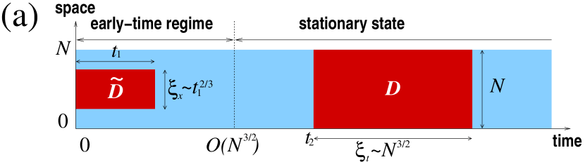
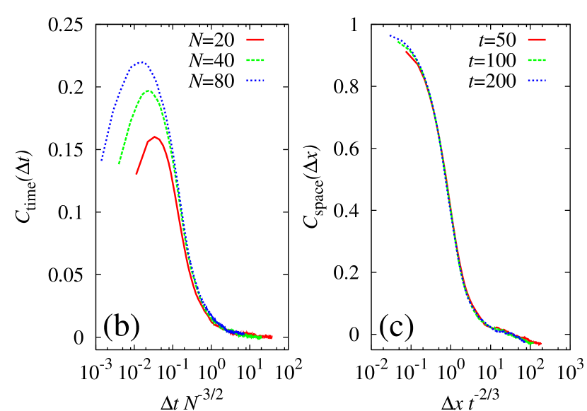
Figure 1: Correlation of the partial height increases. (a) Example of a stationary correlated domain in the stationary state, $D$, and that in the early-time regime, $\tilde{D}$, on both of which all the partial height increases are correlated and the height-steps are uncorrelated. (b) Plot of $C_{\rm time}(\Delta t)$ versus $\Delta tN^{-3/2}$ for the SS model with $\epsilon=1$ and $\rho=1/2$, and the system size $N=20,40$, and $80$. (c) Plot of $C_{\rm space}(\Delta x)$ versus $\Delta xt^{-2/3}$ for the SS model with $\epsilon=1,\rho=1/2,N=10^{4}$ at time $t=50,100$, and $200$.

3 LDF in the early-time regime of the SS model

3.1 Local stationarity

A feature of the stationary state of the one-dimensional KPZ surface is that the height-steps at different sites and at equal or different times are uncorrelated as the fluctuation-dissipation theorem states [10]. On the other hand, the height increases, $\bar{h}(t+\Delta t)-\bar{h}(t)$ with different $t$’s may be correlated. For example, a flat surface has many sites where the heights can increase while in a $V$-shaped surface the heights has only a few such sites. Moreover, such morphological features relevant to the height increase can survive over a certain period of time $\xi_{t}$. The factor $t/N^{3/2}$ in $\mathcal{G}(\gamma,N,t)$ implies that $\xi_{t}\sim N^{3/2}$ [figure 1(a)]. This motivates us to decompose the total height increase $J$ into $t/N^{3/2}$ effectively-independent partial height increases, as $J=\sum_{i=0}^{t/N^{3/2}}J_{iN^{3/2},0}(N^{3/2},N)$, where

$$J_{t,x}(\Delta t,\Delta x)\equiv\sum_{i=x+1}^{x+\Delta x}[h_{i}(t+\Delta t)-h_{i}(t)].$$ (5)

In this notation, $J=J_{0,0}(t,N)$. That such partial height increases are statistically independent is our main assumption. To check its validity we calculate, for the SS model, the normalized correlation defined as

$$C_{\rm time}(\Delta t)=\frac{\langle J_{t,0}(\Delta t,N)\Delta J_{t+\Delta t,0}(\Delta t,N)\rangle_{c}}{\sqrt{\langle J_{t,0}(\Delta t,N)^{2}\rangle_{c}\langle J_{t+\Delta t,0}(\Delta t,N)^{2}\rangle_{c}}}$$ (6)

around $\Delta t\sim N^{3/2}$ where $\langle AB\rangle_{c}=\langle(A-\langle A\rangle)(B-\langle B\rangle)\rangle$. The results shown in figure 1(b) exhibit a rapid decay of the correlation for $\Delta t\gg N^{3/2}$ and confirm the mutual independence of $J_{iN^{3/2},0}(N^{3/2},N)$ with different $i$’s.

In the early-time regime when the roughening is still ongoing, the height-steps at time $t$ are uncorrelated only within each segment of size $\xi_{x}\sim t^{2/3}$, and such locally-stationary segments expand as time goes on and merge into one in the stationary state. At a given time $t_{1}$ with $1\ll t_{1}\ll N^{3/2}$, we may assume that most of the height steps are uncorrelated and all of the partial height increases are correlated within a domain $[0,t_{1}]\times[x,x+\xi_{x}]$ with $\xi_{x}\sim t_{1}^{2/3}$ ($\tilde{D}$ in figure 1(a)), in the same way as within a stationary correlated domain $[t_{2},t_{2}+\xi_{t}]\times[0,N]$ of the stationary state with $\xi_{t}\sim N^{3/2}$ and $t_{2}\gg N^{3/2}$ ($D$ in figure 1(a)). To check this idea, we measure for the SS model the normalized correlation function,

$$C_{\rm space}(\Delta x)=\frac{\langle J_{0,x}(t,\Delta x)J_{0,x+\Delta x}(t,\Delta x)\rangle_{c}}{\sqrt{\langle J_{0,x}(t,\Delta x)^{2}\rangle_{c}\langle J_{0,x+\Delta x}(t,\Delta x)^{2}\rangle_{c}}},$$ (7)

as shown in figure 1(c). The decaying behavior of $C_{\rm space}(\Delta x)$ confirms the mutual independence of the partial height increases, $J_{0,i\xi_{x}}(t,\xi_{x})$ and $J_{0,j\xi_{x}}(t,\xi_{x})$ on different ($i\neq j$) domains of size $t\times\xi_{x}$.

3.2 Dynamic scaling and LDF in the early-time regime of the SS model

The same correlation landscape between the stationary correlated domains of the stationary state and of the early-time regime implies that the characteristic function in the stationary state, $e^{\gamma\langle J\rangle+\mathcal{G}(\gamma,N,t)}$ gives the characteristic function for a stationary correlated domain of the early-time regime, $\langle e^{\gamma J_{0,x}(t,\xi_{x})}\rangle$, provided the system size $N$ in the former is replaced by the correlation length $\xi_{x}\sim\tilde{a}t^{2/3}$ in the latter with $\tilde{a}$ a constant. In this mapping, actual exact functional form of $G(x)$ in equation (2) may possibly change. Then the characteristic function for the early-time height increase is determined as

$$\langle e^{\gamma J}\rangle=\langle e^{\gamma\sum_{i=0}^{N/\xi_{x}}J_{0,i\xi_{x}}(t,\xi_{x})}\rangle\sim\langle e^{\gamma J_{0,x}(t,\xi_{x})}\rangle^{N/\xi_{x}}.$$ (8)

We then have, with $t\ll N^{3/2}$,

$$\langle e^{\gamma J}\rangle=e^{\gamma\langle J\rangle+\tilde{\mathcal{G}}(\gamma,N,t)}\ {\rm with}$$

$$\tilde{\mathcal{G}}(\gamma,N,t)=\frac{N}{\tilde{a}t^{2/3}}\frac{1}{{\tilde{a}}^{3/2}}\frac{\epsilon\sqrt{4\rho(1-\rho)}}{2\sqrt{2\pi}}\times\tilde{G}\left(\sqrt{2\pi}\gamma\sqrt{4\rho(1-\rho)}{\tilde{a}}^{3/2}t\right)$$ (9)

for $\gamma t$ finite with a new function $\tilde{G}(x)$ introduced.

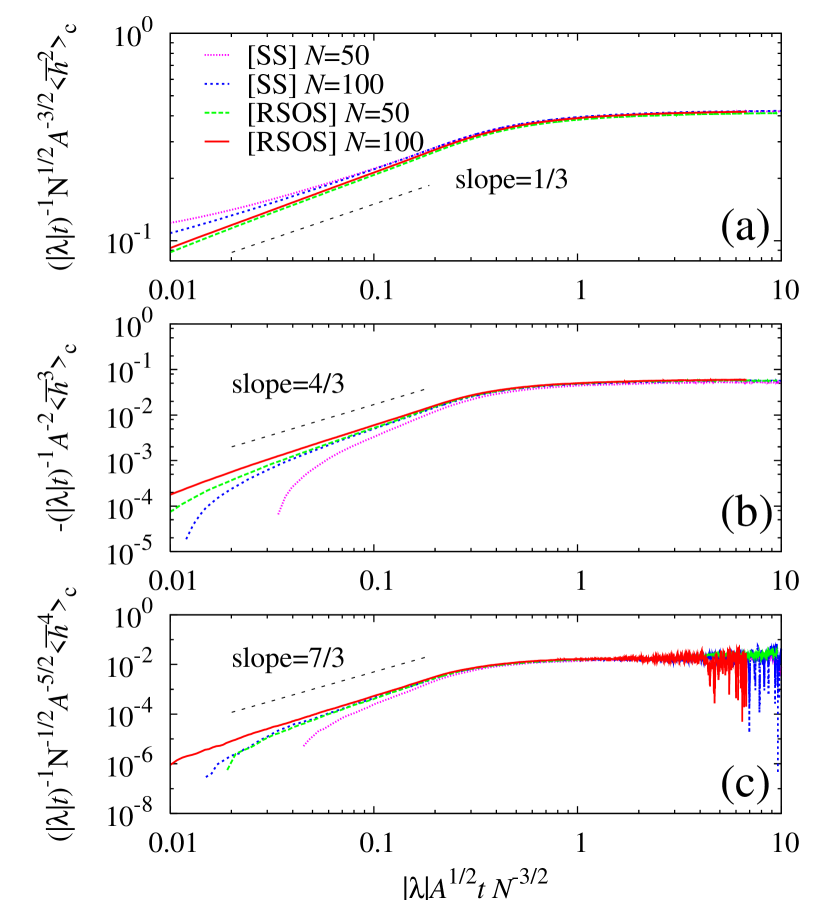
Figure 2: Dynamic scaling of the (a) second, (b) third, and (c) fourth cumulants of the average height of the SS model with $\epsilon=1$ and $\rho=1/2$ ($\lambda=-1,A=1$) and the RSOS model [13] ($\lambda=-0.75,A=0.81$) for $N=50$ and $100$. The data scaled according to equations (10) and (15) are presented, showing good collapse and also confirming the small-$x$ behavior of the scaling functions $\phi_{n}(x)$. The legend is provided in (a).

The expressions of $\mathcal{G}(\gamma,N,t)$ and $\tilde{\mathcal{G}}(\gamma,N,t)$ together determine the dynamic scaling of the average height by the relation $\langle\bar{h}^{n}\rangle_{c}=N^{-n}(\partial^{n}/\partial\gamma^{n})\ln\langle e^{\gamma J}\rangle|_{\gamma=0}$, which yields for $n=2,3,\ldots$,

$$\langle\bar{h}^{n}\rangle_{c}=tN^{(n-3)/2}\epsilon[4\rho(1-\rho)]^{(n+1)/2}\phi_{n}\left(\frac{t}{(N/\tilde{a})^{3/2}}\right)\ {\rm with}$$

$$\phi_{n}(x)\simeq\left\{\begin{array}[]{lc}2^{(n-3)/2}\pi^{(n-1)/2}G^{(n)}(0)&(x\gg 1),\\ 2^{(n-3)/2}\pi^{(n-1)/2}\tilde{G}^{(n)}(0)\ x^{n-5/3}&(x\ll 1).\end{array}\right.$$ (10)

Here $G^{(n)}(0)=(\partial^{n}/\partial z^{n})G(z)|_{z=0}$ and the same for $\tilde{G}^{(n)}(0)$. The scaled data of the $2$nd, $3$rd, and $4$th cumulants in the SS model with $\epsilon=1$ and $\rho=1/2$ are plotted in figure 2, which agree with equation (10).

From equation (9) one also finds that the LDF for $N\gg t^{2/3}$ is given by

$$P(\bar{h}=\langle\bar{h}\rangle+\tilde{y}/t^{1/3})\sim e^{-N\tilde{f}(\tilde{y})}\ {\rm with}$$

$$\tilde{f}(\tilde{y})=\frac{1}{t^{2/3}}\frac{1}{{\tilde{a}}^{5/2}}\frac{\epsilon\sqrt{4\rho(1-\rho)}}{2\sqrt{\pi}}\tilde{H}\left(\frac{\tilde{y}\tilde{a}}{2\epsilon\rho(1-\rho)}\right),$$ (11)

where $\tilde{H}(x)$ is defined by $\tilde{H}=[\tilde{G}(z)-z(\partial/\partial z)\tilde{G}(z)]/\sqrt{2}$ and $x=(\partial/\partial z)\tilde{G}(z)$.

4 Scaling analysis and universal LDF

The LDF and the dynamic scaling behaviors shown in equations (10) and (11) can be represented in terms of the parameters of the KPZ equation (1), which enables us to check their universality. Following the procedures proposed in Ref. [14], one finds the following dimensionless variables

$$h^{\prime}=\frac{\lambda}{2\nu}h,\ \ x^{\prime}=\frac{\lambda^{2}D}{2\nu^{3}}x,\ \ \tau=\frac{\lambda^{4}D^{2}}{4\nu^{5}}t$$ (12)

satisfy an equation without parameters, $(\partial/\partial\tau)h^{\prime}=(\partial^{2}/\partial x^{2})h^{\prime}+(\partial h/\partial x)^{2}+\eta^{\prime}(x^{\prime},\tau)$ with $\langle\eta^{\prime}(x_{1}^{\prime},\tau_{1})\eta^{\prime}(x_{2}^{\prime},\tau_{2})\rangle=\delta(x_{1}^{\prime}-x_{2}^{\prime})\delta(\tau_{1}-\tau_{2})$. Therefore both $\mathcal{G}$ and $\tilde{\mathcal{G}}$ should be functions of $\gamma N(\lambda/\nu)$ (for $\gamma J$), $(\lambda^{2}D/\nu^{3})N$, and $(\lambda^{4}D^{2}/\nu^{5})t$. Keeping the $t$ and $N$ dependence appearing in equations (2) and (9), those functions turn out to be given by

$$\mathcal{G}(\gamma,N,t)=|\lambda|\sqrt{A}\frac{t}{N^{3/2}}\mathcal{B}\left({\rm sign}(\lambda)\sqrt{A}\gamma\,N^{3/2}\right),$$ (13)

where $A\equiv D/\nu$, and

$$\tilde{\mathcal{G}}(\gamma,N,t)=\frac{1}{|\lambda|^{2/3}A^{1/3}}\frac{N}{t^{2/3}}\tilde{\mathcal{B}}\left(\lambda A\gamma\,t\right).$$ (14)

Here, $\mathcal{B}(x)$ and $\tilde{\mathcal{B}}(x)$ are the scaling functions to be identified as follows. The nonlinear term with the parameter $\lambda$ in equation (1) has been introduced to describe the lateral growth and thus $\lambda=(\partial^{2}/\partial u^{2})(\partial/\partial t)\langle\bar{h}\rangle|_{u=0}$ with $u$ the average slope of the surface [15], which leads to $\lambda=-\epsilon$ for the SS model where $\langle\bar{h}\rangle=2\epsilon\rho(1-\rho)t$ and $u=1-2\rho$. Also, the uncorrelated height-steps in the stationary state result in $\langle(h_{i}(t)-h_{j}(t))^{2}\rangle_{c}\sim A|i-j|$ [16], which gives $A=4\rho(1-\rho)$ from the comparison with the exact solution for the SS model [17]. Substituting these values to equation (13), one finds that equations (2) and (13) perfectly agree with each other under the relation $\mathcal{B}(x)=G(-\sqrt{2\pi}x)/(2\sqrt{2\pi})$. Also equations (9) and (14) become equal under the relation $\tilde{a}=|\lambda|^{2/3}A^{1/3}\tilde{c}$ with $\tilde{c}$ an universal constant and the identity $\tilde{\mathcal{B}}(x)=\tilde{G}(-\sqrt{2\pi}x\tilde{c}^{3/2})/(2\sqrt{2\pi}\tilde{c}^{5/2})$.

With the functions $\mathcal{G}$ and $\tilde{\mathcal{G}}$ in equations (13) and (14), we find

$$\langle\bar{h}^{n}\rangle_{c}=tN^{(n-3)/2}|\lambda|A^{(n+1)/2}\phi_{n}\left(|\lambda|A^{1/2}\frac{t}{N^{3/2}}\tilde{c}^{3/2}\right).$$ (15)

To check the $\lambda$ and $A$ dependence in equation (15) and thereby explore the universal scaling function $\phi_{n}(x)$, we performed numerical simulations of the RSOS model [13], where the flat surface, $h_{i}=0$ for all $i$ at $t=0$, grows via the integer-valued height at a randomly-chosen site being increased by $1$ with probability $1$ unless the new height differs from neighboring heights by larger than $1$. The numerical estimates have shown that $\lambda\simeq-0.75$ and $A\simeq 0.81$ for the RSOS model [15]. Using these values, we plot the scaled data of the $n$th cumulants with $n=2,3,$ and $4$ obtained from the RSOS model together with those from the SS model ($\epsilon=1$ and $\rho=1/2$) in figure 2. The good collapse of those data obtained for different times and system sizes strongly supports the existence of the universal scaling function $\phi_{n}(x)$.

Figure 3: Universal LDF in the early-time regime. The data scaled according to equation (17) are shown, obtained from the simulations of the SS model ($\epsilon=1$ and $\rho=1/2$) and the RSOS model with $N=100$ and $200$ and $t=20$ and $60$. The collapsed data show the universal function $(2\sqrt{\pi}\tilde{c}^{5/2})^{-1}\tilde{H}(2\tilde{c}x)$ in equation (17). To compare the functions $H(x)$ and $\tilde{H}(x)$, we draw the curve representing the function $H(2x\tilde{c})/(2\pi^{1/2}\tilde{c}^{5/2})$ with $\tilde{c}=1.2$ chosen for the best fitting.

The Legendre transformations of equations (13) and (14) give the LDF as

$$f(y)=\frac{1}{N^{3/2}}|\lambda|\sqrt{A}\frac{1}{2\sqrt{\pi}}H\left(-2\frac{y}{\lambda A}\right)$$ (16)

for the stationary state and

$$\tilde{f}(\tilde{y})=\frac{1}{t^{2/3}}\frac{1}{|\lambda|^{2/3}A^{1/3}}\frac{1}{2\sqrt{\pi}\tilde{c}^{5/2}}\tilde{H}\left(-2\tilde{c}\,{\rm sign}(\lambda)\frac{\tilde{y}}{|\lambda|^{1/3}A^{2/3}}\right)$$ (17)

for the early-time regime, respectively. While the acquisition of the data for the LDF of the stationary state is hampered by long evolution times, that of the early-time regime can be obtained within reasonable times. We plot $|\lambda|^{2/3}A^{1/3}t^{2/3}N^{-1}\ln[P(\bar{h})/P(\langle\bar{h}\rangle)]$ versus $|\lambda|^{-1/3}A^{-2/3}t^{-1/3}(\bar{h}-\langle\bar{h}\rangle)$ with different system sizes and times in the SS model and the RSOS model in figure 3, which shows clearly a universal curve $(2\sqrt{\pi}\tilde{c}^{5/2})^{-1}\tilde{H}(2\tilde{c}x)$. Note that $\lambda$ is negative for both models.

Contrary to the stationary state, the exact functional form of the universal LDF of the early-time regime is not known yet since all the eigenstates of the time-evolution operator are involved in the characteristic function. From the physics viewpoint, the detailed functional form of the probability distribution of the sum of correlated variables is expected to depend not only on the type of correlation but also on the type of the boundary condition [6]. Since the exact universal LDF of the stationary state has been obtained under the periodic boundary condition, it is not possible to draw the conclusion that $H(x)=\tilde{H}(x)$ on the analytical basis. The boundary condition for the locally-stationary segment in the early-time regime is not obvious. On the one hand, however, the functions $H(x)$ and $\tilde{H}(x)$ are expected to display similar behaviors due to the same type of correlations among height increases and as seen in figure 3, the function $\tilde{H}(x)$ has indeed asymmetric tails as $H(x)$ does. Moreover, we compare $H(x)$ and $\tilde{H}(x)$ in figure 3 by drawing the curve representing the function $(2\sqrt{\pi}\tilde{c}^{5/2})^{-1}H(2x\tilde{c})$ with $\tilde{c}=1.2$ chosen for the best fitting. The analytic curve and the numerical one are in good agreement over the whole range of data presented. This is consistent with a conjecture that $H(x)$ = $\tilde{H}(x)$.

5 Conclusion

We have investigated the statistics of the average height for the one-dimensional KPZ surface. The LDF in the stationary state implies that the average height is decomposed into statistically-independent components each of which is a set of correlated variables, and we checked its validity. To derive the LDF in the early-time regime, we assumed that the statistics of the average height in such a component remains the same across both time regimes, in that the scaling property and the model-parameter dependence of the characteristic function are not changed. The scaling analysis of the KPZ equation enables us to find the equation-parameter dependence of the LDF. Using this result in analyzing the simulation data obtained for two different models, we confirmed the universality of the LDF.

We combined the exact results and the scaling analysis to explore the universality of the LDF, which can be complementary to the measurement of the cumulants’ ratio. The exact functional form of the universal LDF is an open question. Given that little is known about the statistical properties of non-stationary systems, the present work could stimulate related research including the investigation of the fluctuations in non-stationary systems.

References

References

- [1] Kardar M, Parisi G and Zhang Y 1986 Phys. Rev. Lett. 56 889
- [2] Barabási A L and Stanley H 1995 Fractal Concepts in Surface Growth (Cambridge: Cambridge University Press)
- [3] Derrida B and Lebowitz J 1998 Phys. Rev. Lett. 80 209
- [4] Derrida B and Appert C 1999 J. Stat. Phys. 94 1
- [5] Lee D S and Kim D 1999 Phys. Rev. E 59 6476
- [6] Appert C 2000 Phys. Rev. E 61 2092
- [7] Plischke M, Rácz Z and Liu D 1987 Phys. Rev. B 35 3485
- [8] Gallavotti G and Cohen E G D 1995 Phys. Rev. Lett. 74 2694
- [9] Lebowitz J L and Spohn H 1999 J. Stat. Phys. 95 333
- [10] Halpin-Healy T and Zhang Y C 1995 Phys. Rep. 254 215
- [11] Gwa L H and Spohn H 1992 Phys. Rev. Lett. 68 725
- [12] Kim D 1995 Phys. Rev. E 52 3512
- [13] Kim J and Kosterlitz J 1989 Phys. Rev. Lett. 62 2289
- [14] Amar J G and Family F 1992 Phys. Rev. A 45
- [15] Krug J, Meakin P and Halpin-Healy T 1999 Phys. Rev. A 45 638
- [16] Huse D A, Henley C L and Fisher D S 1985 Phys. Rev. Lett. 55 2924
- [17] Derrida B and Mallick K 1997 J. Phys. A 30 1031