A modified triplet-wave expansion method applied to the alternating Heisenberg chain

Abstract

An alternative triplet-wave expansion formalism for dimerized spin systems is presented, a modification of the ‘bond operator’ formalism of Sachdev and Bhatt. Projection operators are used to confine the system to the physical subspace, rather than constraint equations. The method is illustrated for the case of the alternating Heisenberg chain, and comparisons are made with the results of dimer series expansions and exact diagonalization. Some discussion is included of the phenomenon of “quasiparticle breakdown”, as it applies to the two-triplon bound states in this model.

I INTRODUCTION

There has been much interest recently in the phenomenon of dimerization in $S=1/2$ Heisenberg antiferromagnets, where pairs of neighbouring spins couple to form $S=0$ singlet dimers. The dimerization may arise due to inhomogeneous bond interactions, as in the alternating Heisenberg chain (AHC) model, or the Shastry-Sutherland model in two dimensions shastry1981 . Alternatively, it may emerge spontaneously, as the result of frustration lhuillier2001 : this seems to occur in the J₁-J₂ square lattice model at intermediate coupling values, for instance, although there is disagreement as to whether the pattern of dimerization is ordered (‘valence bond solid’) read1991 ; kotov1999 or disordered (‘valence bond liquid’ or ‘resonating valence bond’) anderson1987 ; capriotti2003 .

To understand the properties of dimerized phases, it is useful to construct an appropriate lattice formalism describing the dimers and their spin-triplet excitations. The physics of the system can then be connected with the properties of the elementary triplet excitations; and one can also use the formalism to construct a continuum ‘effective Lagrangian’ field theory for the system at hand. Such a formalism was the ‘bond-operator’ representation constructed by Sachdev and Bhatt sachdev1990 (see also Chubukov chubukov1989 ) some years ago, which is analogous to the spin-wave representation traditionally used to describe the magnetically ordered phases of these systems mattis1981 .

Sachdev and Bhatt sachdev1990 considered two spins ${\bf S_{1}}$ and ${\bf S_{2}}$ at either end of a single bond on the lattice, forming a dimer. They introduced a singlet and three triplet boson creation operators to form the corresponding states from the vacuum:

$$|s> = s^{\dagger}|0>=\frac{1}{\sqrt{2}}(|\uparrow\downarrow>-|\downarrow\uparrow>)$$

$$|t_{x}> = t^{\dagger}_{x}|0>=-\frac{1}{\sqrt{2}}(|\uparrow\uparrow>-|\downarrow\downarrow>)$$

$$|t_{y}> = t_{y}^{\dagger}|0>=\frac{i}{\sqrt{2}}(|\uparrow\uparrow>+|\downarrow\downarrow>)$$

$$|t_{z}> = t_{z}^{\dagger}|0>=\frac{1}{\sqrt{2}}(|\uparrow\downarrow>+|\downarrow\uparrow>)$$ (1)

Then the spin operators can be represented

$$S_{1\alpha} = \frac{1}{2}[s^{\dagger}t_{\alpha}+t_{\alpha}^{\dagger}s-i\epsilon_{\alpha\beta\gamma}t^{\dagger}_{\beta}t_{\gamma}]$$

$$S_{2\alpha} = \frac{1}{2}[-s^{\dagger}t_{\alpha}-t_{\alpha}^{\dagger}s-i\epsilon_{\alpha\beta\gamma}t^{\dagger}_{\beta}t_{\gamma}]$$ (2)

(where $\alpha,\beta,\gamma$ take values $x,y$ or $z$), with the constraint that physical states must satisfy

$$s^{\dagger}s+t^{\dagger}_{\alpha}t_{\alpha}=1.$$ (3)

They applied this formalism to develop a mean field theory of the frustrated square-lattice antiferromagnet.

The problem with this approach is that the constraint (3) is awkward to implement analytically. Kotov et al. kotov1998 have applied an alternative “Brueckner approach”, in which the singlet operator is discarded, leaving only the constraint that two triplet excitations are not allowed on the same site (bond). This is implemented by an infinite on-site repulsion term between triplets, which is applied using an analytic Brueckner approach, valid when the density of triplets is small. The approach has been applied to the two-layer Heisenberg model kotov1998 ; shevchenko1999 , the quantum spin-ladder sushkov1998 ; kotov1999a , and the dimerized Heisenberg chain with frustration shevchenko1999a , and some useful physical insights have been obtained. In particular, the occurrence of two-particle bound states formed from the elementary triplet excitations seems to be generic in these models. Nevertheless, the Brueckner implementation of the on-site repulsion term is also somewhat awkward to apply, and difficult to carry through in higher orders.

Here we present an alternative approach in which the triplet exclusion constraint is implemented automatically by means of projection operators. We also use a “modified” formalism, analogous to modified spin-wave theory takahashi1987 ; gochev1994 , in which the two-body terms in the Hamiltonian are diagonalized through to the highest order calculated. The absence of any constraint makes the formalism easier and more transparent to apply. The only drawback is the appearance of extra many-body interaction terms in the Hamiltonian, so that carrying the calculation to high orders would require the aid of a computer.

To illustrate the formalism, we apply it to the case of the alternating Heisenberg chain (AHC). This model has itself attracted much attention recently, as new materials such as Cu(NO${}_{3})_{2}$.2.5D₂O xu2000 ; tennant2002 have been constructed which appear to conform to this simple model, while at the same time more powerful neutron scattering facilities are coming on-line to explore their properties. For a review and further references, see Barnes et al. barnes1999 . On the theoretical side, Uhrig and Schulz uhrig1996 used a field theory approach to predict the appearance of both singlet ($S=0$) and triplet ($S=1$) bound states below the two-triplet continuum. This was confirmed by later studies fledderjohann1997 ; bouzerar1998 ; shevchenko1999a . Bouzerar and Sil bouzerar1998a and Shevchenko et al. shevchenko1999a have treated the AHC using the Brueckner approach; while Singh and Zheng singh1999 , Trebst et al. trebst2000 and Zheng et al. zheng2003 have carried out high-order dimer series expansions for the model, which give an accurate numerical picture of the dimerized phase.

In Section II, we lay out the triplet-wave expansion formalism for the case of the alternating chain. In Section III, the expansion to leading orders on powers of the coupling $\lambda$ is discussed for the ground state energy and energy gap. In Section IV, numerical results are presented for the ground-state energy, the one-particle spectrum, the two-triplon bound states, and the exclusive structure factors for these states. A summary and conclusions are presented in Section V.

II Triplet-wave expansion

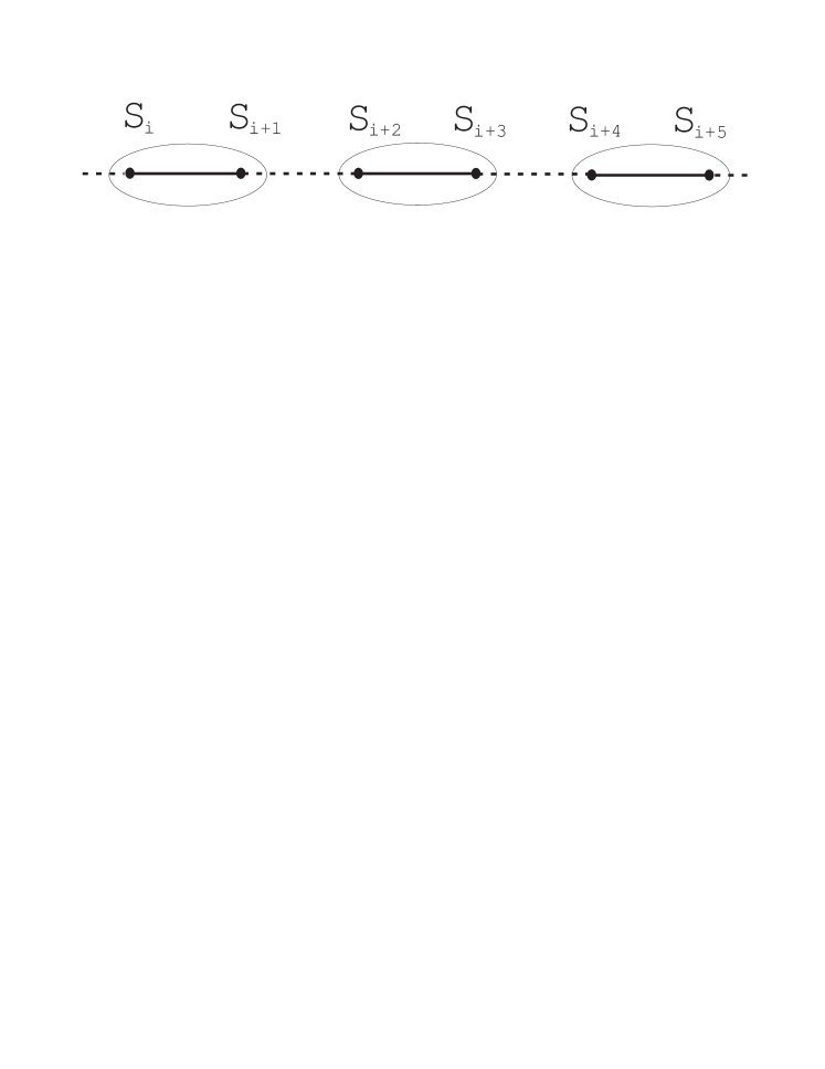
Figure 1: The alternating Heisenberg chain.

The Hamiltonian for the alternating Heisenberg chain can be written

$$H=\sum_{i\ odd}{\bf S_{i}\cdot S_{i+1}}+\lambda\sum_{i\ even}{\bf S_{i}\cdot S_{i+1}}$$ (4)

For $\lambda=0$, the system reduces to independent dimers as shown in Figure 1. Let us consider a single dimer with two spins ${\bf S_{1},S_{2}}$. The four states in the Hilbert space consist of a singlet and three triplet states with total spin $S=0,1$ respectively, and eigenvalues

$${\bf S_{1}\cdot S_{2}}=\left\{\begin{array}[]{cc}-3/4&(S=0)\\ +1/4&(S=1)\end{array}\right.$$ (7)

We denote the singlet ground state as $|0>$, and introduce triplet creation operators that create the triplet states out of the vacuum $|0>$, as follows

$$|0> = \frac{1}{\sqrt{2}}[|\uparrow\downarrow>-|\downarrow\uparrow>]$$

$$|1,x> = t^{\dagger}_{x}|0>=-\frac{1}{\sqrt{2}}[|\uparrow\uparrow>-|\downarrow\downarrow>]$$

$$|1,y> = t^{\dagger}_{y}|0>=\frac{i}{\sqrt{2}}[|\uparrow\uparrow>+|\downarrow\downarrow>]$$

$$|1,z> = t^{\dagger}_{z}|0>=\frac{1}{\sqrt{2}}[|\uparrow\downarrow>+|\downarrow\uparrow>]$$ (8)

Then the spin operators ${\bf S_{1}}$ and ${\bf S_{2}}$ can be represented in terms of triplet operators by

$$S_{1\alpha} = \frac{1}{2}[t^{\dagger}_{\alpha}(1-t^{\dagger}_{\gamma}t_{\gamma})+(1-t^{\dagger}_{\gamma}t_{\gamma})t_{\alpha}-i\epsilon_{\alpha\beta\gamma}t^{\dagger}_{\beta}t_{\gamma}]$$

$$S_{2\alpha} = \frac{1}{2}[-t^{\dagger}_{\alpha}(1-t^{\dagger}_{\gamma}t_{\gamma})-(1-t^{\dagger}_{\gamma}t_{\gamma})t_{\alpha}$$ (9)

$$-i\epsilon_{\alpha\beta\gamma}t^{\dagger}_{\beta}t_{\gamma}]$$

where $\alpha,\beta,\gamma$ take the values $x,y,z$ and repeated indices are summed over. This is similar to the representation of Sachdev and Bhatt sachdev1990 , except that we have omitted singlet operators $s^{\dagger},s$, but used projection operators $(1-t^{\dagger}_{\gamma}t_{\gamma})$ instead. Assume the triplet operators obey bosonic commutation relations

$$[t_{\alpha},t^{\dagger}_{\beta}]=\delta_{\alpha\beta},$$ (10)

then one can show that within the physical subspace (i.e. total number of triplet states is 0 or 1), the representation (9) obeys the correct spin operator algebra

$$[S_{1\alpha},S_{1\beta}]=i\epsilon_{\alpha\beta\gamma}S_{1\gamma},\hskip 14.22636pt[S_{2\alpha},S_{2\beta}]=i\epsilon_{\alpha\beta\gamma}S_{2\gamma},$$ (11)

$$[S_{1\alpha},S_{2\beta}]=0$$ (12)

$${\bf S}_{1}^{2}={\bf S}_{2}^{2}=3/4,\hskip 14.22636pt{\bf S_{1}\cdot S_{2}}=t^{\dagger}_{\alpha}t_{\alpha}-3/4$$ (13)

The projection operators ensure that we remain within the subspace.

Returning to the alternating chain, we can now define triplet operators $t^{\dagger}_{n\alpha},t_{n\alpha}$ for each dimer $n$ along the chain. For a chain of $N$ dimers, the Hamiltonian now can be expressed in terms of triplet operators as

$$H = -\frac{3N}{4}+\sum_{n}t^{\dagger}_{n\alpha}t_{n\alpha}-\frac{\lambda}{4}\sum_{n}\{t^{\dagger}_{n\alpha}(1-t^{\dagger}_{n\gamma}t_{n\gamma})t^{\dagger}_{n+1,\alpha}(1-t^{\dagger}_{n+1,\delta}t_{n+1,\delta})+(1-t^{\dagger}_{n\gamma}t_{n\gamma})t_{n\alpha}(1-t^{\dagger}_{n+1,\delta}t_{n+1,\delta})t_{n+1,\alpha}$$ (14)

$$+t^{\dagger}_{n\alpha}(1-t^{\dagger}_{n\gamma}t_{n\gamma})(1-t^{\dagger}_{n+1,\delta}t_{n+1,\delta})t_{n+1,\alpha}+(1-t^{\dagger}_{n\gamma}t_{n\gamma})t_{n\alpha}t^{\dagger}_{n+1,\alpha}(1-t^{\dagger}_{n+1,\delta}t_{n+1,\delta})\}$$

$$+\frac{\lambda}{4}\sum_{n}t^{\dagger}_{n\beta}t_{n\gamma}(t^{\dagger}_{n+1,\gamma}t_{n+1,\beta}-t^{\dagger}_{n+1,\beta}t_{n+1,\gamma})+i\frac{\lambda}{4}\epsilon_{\alpha\beta\gamma}\sum_{n}\{t^{\dagger}_{n\alpha}(1-t^{\dagger}_{n\delta}t_{n\delta})t^{\dagger}_{n+1,\beta}t_{n+1,\gamma}$$

$$-t^{\dagger}_{n\beta}t_{n\gamma}t^{\dagger}_{n+1,\alpha}(1-t^{\dagger}_{n+1,\delta}t_{n+1.\delta})+(1-t^{\dagger}_{n\delta}t_{n\delta})t_{n\alpha}t^{\dagger}_{n+1,\beta}t_{n+1,\gamma}-t^{\dagger}_{n\beta}t_{n\gamma}(1-t^{\dagger}_{n+1,\delta}t_{n+1,\delta})t_{n+1,\alpha}\}$$

This expression includes terms containing up to 6 triplet operators. For the purposes of the present calculations, we shall drop terms with more than 4 triplet operators henceforwards.

Next, perform a Fourier transform

$$t_{k\alpha} = (\frac{1}{N})^{1/2}\sum_{n}e^{ikn}t_{n\alpha}$$

$$t^{\dagger}_{k\alpha} = (\frac{1}{N})^{1/2}\sum_{n}e^{-ikn}t^{\dagger}_{n\alpha}$$ (15)

(we set the spacing between dimers $d=1$), then the Hamiltonian becomes

$$H = -\frac{3N}{4}+\sum_{k}t^{\dagger}_{k\alpha}t_{k\alpha}-\frac{\lambda}{4}\sum_{k}\cos k[t^{\dagger}_{k\alpha}t^{\dagger}_{-k\alpha}+t_{k\alpha}t_{-k\alpha}+2t^{\dagger}_{k\alpha}t_{k\alpha}]+\frac{\lambda}{2\sqrt{N}}\epsilon_{\alpha\beta\gamma}\sum_{123}\delta_{1+2-3}\sin k_{1}[t^{\dagger}_{1\alpha}t^{\dagger}_{2\beta}t_{3\gamma}$$ (16)

$$+t^{\dagger}_{3\gamma}t_{1\alpha}t_{2\beta}]+\frac{\lambda}{2N}\sum_{1234}\{\delta_{1+2+3-4}t^{\dagger}_{1\alpha}t^{\dagger}_{2\alpha}t^{\dagger}_{3\gamma}t_{4\gamma}\cos k_{1}+\delta_{1-2-3-4}t^{\dagger}_{1\gamma}t_{2\gamma}t_{3\alpha}t_{4\alpha}\cos k_{4}$$

$$+\delta_{1+2-3-4}[t^{\dagger}_{1\alpha}t^{\dagger}_{2\gamma}t_{3\gamma}t_{4\alpha}\cos k_{4}+t^{\dagger}_{1\alpha}t^{\dagger}_{2\gamma}t_{3\gamma}t_{4\alpha}\cos k_{1}]\}$$

$$+\frac{\lambda}{4N}\sum_{1234}\delta_{1+2-3-4}[t^{\dagger}_{1\gamma}t^{\dagger}_{2\beta}t_{3\beta}t_{4\gamma}-t^{\dagger}_{1\beta}t^{\dagger}_{2\beta}t_{3\gamma}t_{4\gamma}]\cos(k_{1}-k_{3})$$

Finally, as in a standard spin-wave analysis, we perform a Bogoliubov transform

$$t_{k\alpha}=c_{k}\tau_{k\alpha}+s_{k}\tau^{\dagger}_{-k\alpha}$$ (17)

where $c_{k}=\cosh\theta_{k}$, $s_{k}=\sinh\theta_{k}$, $\theta_{-k}=\theta_{k}$, which preserves the boson commutation relations

$$[\tau_{k\alpha},\tau^{\dagger}_{k^{\prime}\beta}]=\delta_{kk^{\prime}}\delta_{\alpha\beta}$$ (18)

and is intended to diagonalize the Hamiltonian up to quadratic terms. After normal ordering, the transformed Hamiltonian up to fourth order terms reads

$$H=W_{0}+H_{2}+H_{3}+H_{4}.$$ (19)

Here the constant term is

$$W_{0} = 3N[-\frac{1}{4}+R_{2}$$ (20)

$$-\frac{\lambda}{2}(R_{3}+R_{4})(1-8R_{2}-2R_{1}+R_{3}-R_{4})]$$

expressed in terms of the momentum sums

$$R_{1} = \frac{1}{N}\sum_{k}c_{k}s_{k}$$

$$R_{2} = \frac{1}{N}\sum_{k}s_{k}^{2}$$

$$R_{3} = \frac{1}{N}\sum_{k}c_{k}s_{k}\cos k$$

$$R_{4} = \frac{1}{N}\sum_{k}s_{k}^{2}\cos k$$ (21)

The quadratic terms are

$$H_{2}=\sum_{k,\alpha}[E_{k}\tau^{\dagger}_{k\alpha}\tau_{k\alpha}+Q_{k}(\tau_{k\alpha}\tau_{-k\alpha}+\tau^{\dagger}_{k\alpha}\tau^{\dagger}_{-k\alpha})]$$ (22)

where

$$E_{k}=(c_{k}^{2}+s_{k}^{2})[1+4\lambda(R_{3}+R_{4})-\frac{\lambda}{2}\cos k(1-2R_{1}-8R_{2}-2R_{4})]-\lambda c_{k}s_{k}[\cos k(1-8R_{2}-2R_{1}+2R_{3})-2(R_{3}+R_{4})]$$ (23)

$$Q_{k}=c_{k}s_{k}[1-\frac{\lambda}{2}(\cos k(1-2R_{1}-8R_{2}-2R_{4})-8(R_{3}+R_{4}))-\frac{\lambda}{4}(c_{k}^{2}+s_{k}^{2})[\cos k(1-8R_{2}-2R_{1}+2R_{3})-2(R_{3}+R_{4})]$$ (24)

The third and fourth-order terms are

$$H_{3}=\frac{\lambda}{2\sqrt{N}}\epsilon_{\alpha\beta\gamma}\sum_{123}[\delta_{1+2+3}\Phi^{(1)}_{3}(\tau_{1\alpha}\tau_{2\beta}\tau_{3\gamma}+\tau^{\dagger}_{3\gamma}\tau^{\dagger}_{2\beta}\tau^{\dagger}_{1\alpha})+\delta_{1+2-3}\Phi^{(2)}_{3}(\tau^{\dagger}_{1\alpha}\tau^{\dagger}_{2\beta}\tau_{3\gamma}+\tau^{\dagger}_{3\gamma}\tau_{2\beta}\tau_{1\alpha})]$$ (25)

and

$$H_{4} = \frac{\lambda}{4N}\sum_{1234}[\delta_{1+2+3+4}\Phi^{(1)}_{4}(\tau^{\dagger}_{1\alpha}\tau^{\dagger}_{2\alpha}\tau^{\dagger}_{3\gamma}\tau^{\dagger}_{4\gamma}+\tau_{1\alpha}\tau_{2\alpha}\tau_{3\gamma}\tau_{4\gamma})+\delta_{1+2-3-4}(\Phi^{(2)}_{4}\tau^{\dagger}_{1\alpha}\tau^{\dagger}_{2\alpha}\tau_{3\gamma}\tau_{4\gamma}+\Phi_{4}^{(3)}\tau^{\dagger}_{1\alpha}\tau^{\dagger}_{2\gamma}\tau_{3\alpha}\tau_{4\gamma})$$ (26)

$$+\delta_{1+2+3-4}\Phi^{(4)}_{4}(\tau^{\dagger}_{1\alpha}\tau^{\dagger}_{2\alpha}\tau^{\dagger}_{3\gamma}\tau_{4\gamma}+\tau^{\dagger}_{4\gamma}\tau_{3\gamma}\tau_{2\alpha}\tau_{1\alpha})]$$

where we have used the shorthand notation $1\cdots 4$ for momenta $k_{1}\cdots k_{4}$, and the vertex functions $\Phi^{(i)}_{3},\Phi^{(i)}_{4}$ are listed in Appendix A.

The condition that the off-diagonal quadratic terms vanish is

$$Q_{k}=0.$$ (27)

In a conventional spin-wave approach, this would be implemented in leading order only, giving the condition

$$\tanh 2\theta_{k}=\frac{2c_{k}s_{k}}{c_{k}^{2}+s_{k}^{2}}=\frac{\lambda\cos k}{2[1-\lambda/2\cos k]}$$ (28)

This would leave some residual off-diagonal quadratic terms, arising from the normal-ordering of quartic operators. In a ‘modified’ approach gochev1994 , we demand that these terms vanish entirely up to the order calculated, giving the modified condition

$$\tanh 2\theta_{k}=\frac{\lambda[\cos k(1-8R_{2}-2R_{1}+2R_{3})-2(R_{3}+R_{4})]}{2[1-\lambda\cos k(1-2R_{1}-8R_{2}-2R_{4})/2+4\lambda(R_{3}+R_{4})]}$$ (29)

Self-consistent solutions for the N equations (29), with the four parameters $R_{1}\cdots R_{4}$ given by equation (21), can easily be found by numerical means, starting from the conventional result (28).

III Expansion in powers of $\lambda$

As a first check on the formalism, one may calculate the leading terms in an expansion of the energy eigenvalues in powers of $\lambda$. From equation (28), we easily see that to order $\lambda^{2}$

$$s_{k} = \frac{\lambda}{4}\cos k+\frac{\lambda^{2}}{8}\cos^{2}k$$

$$c_{k} = 1+\frac{\lambda^{2}}{32}\cos^{2}k$$ (30)

and hence the lattice sums (21) can be evaluated

$$R_{1} = \frac{\lambda^{2}}{16},\hskip 14.22636ptR_{2}=\frac{\lambda^{2}}{32},$$

$$R_{3} = \frac{\lambda}{8}+O(\lambda^{3}),\hskip 14.22636ptR_{4}=O(\lambda^{3})$$ (31)

The leading-order behaviour of the vertex functions may easily be deduced from Appendix A.

Substituting in equation (20), the ground state energy per site is

$$\epsilon_{0} = \frac{W_{0}}{2N}=\frac{3}{2}\left[-\frac{1}{4}+R_{2}-\frac{\lambda}{2}(R_{3}+R_{4})(1-8R_{2}\right.$$ (32)

$$\left.-2R_{1}+R_{3}-R_{4})\right]$$

$$\sim -\frac{3}{8}-\frac{3\lambda^{2}}{64}-\frac{3\lambda^{3}}{256}+O(\lambda^{4}),\hskip 14.22636pt\lambda\rightarrow 0$$

in agreement with dimer series expansion results previously obtained for this model singh1999 . One can easily show that perturbation diagrams such as those in Figure 2 do not contribute until $O(\lambda^{4})$ or higher.

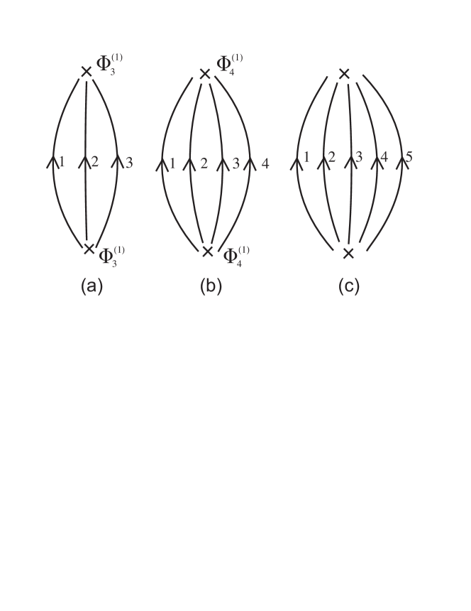
Figure 2: Perturbation diagrams contributing to the ground-state energy.

The energy gap at leading order can be found from equation (23):

$$E_{k}\sim 1-\frac{\lambda}{2}\cos k+\frac{\lambda^{2}}{8}[4-\cos^{2}k],\hskip 14.22636pt\lambda\rightarrow 0$$ (33)

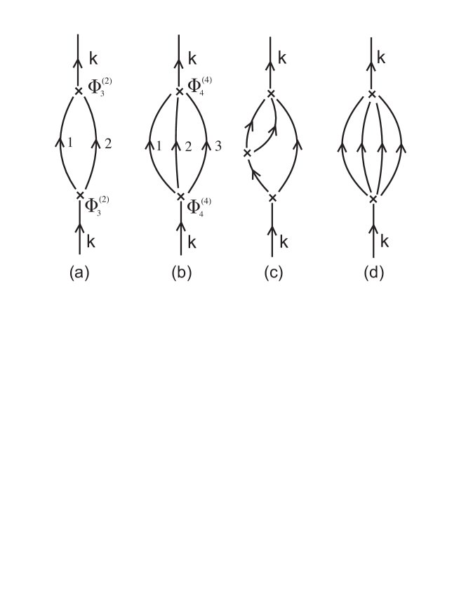
Figure 3: Perturbation diagrams contributing to the one-particle energy.

The perturbation diagrams Figures 3a) and 3b) also contribute at order $\lambda^{2}$. Note that diagram 3b) does not appear in the formalism of Shevchenko et al. shevchenko1999a ; the extra terms in our formalism are needed to implement the hardcore constraint that two triplons cannot occupy the same site. At leading order, the contributions of these diagrams are

$$\Delta E_{k}^{3a)}\sim-\frac{\lambda^{2}}{4}(1+\cos k),\hskip 14.22636pt\lambda\rightarrow 0$$ (34)

$$\Delta E_{k}^{3b)}\sim-\frac{\lambda^{2}}{4},\hskip 14.22636pt\lambda\rightarrow 0$$ (35)

(see the next section for further details). This gives a total single-particle energy

$$\epsilon_{k}\sim 1-\frac{\lambda}{2}\cos k-\frac{\lambda^{2}}{8}\cos k[2+\cos k],\hskip 14.22636pt\lambda\rightarrow 0$$ (36)

which again agrees with series expansion results singh1999 .

If we compare equation (36) at small momentum with the continuum dispersion relation for a free boson,

$$\epsilon_{k}\sim\sqrt{m^{2}c^{4}+k^{2}c^{2}}$$ (37)

we readily discover the leading behaviour of the effective triplon parameters, i.e. the triplon mass

$$m\sim\frac{2}{\lambda}[1+\lambda+O(\lambda^{2})]$$ (38)

and the ‘speed of light’

$$c\sim\frac{\lambda}{2}-\frac{3\lambda^{2}}{8}+O(\lambda^{3})$$ (39)

in lattice units. Note that the mass diverges and the speed of light vanishes as $\lambda\rightarrow 0$.

IV Numerical Results

Writing the Hamiltonian as

$$H=H_{0}+V$$ (40)

where

$$H_{0}=W_{0}+H_{2}$$ (41)

and

$$V=H_{3}+H_{4}$$ (42)

we can treat $H_{0}$ as the unperturbed Hamiltonian and $V$ as a perturbation to obtain the leading-order corrections to the predictions for physical quantities outlined in the previous section. Numerical results for the model have been obtained using the finite-lattice method. The momentum sums are carried out for a fixed number of dimers $N$, using corresponding discrete values for the momentum $k$, e.g.

$$k_{n}=\frac{2\pi n}{N},\hskip 14.22636ptn=1.\cdots N$$ (43)

Results were obtained for $N$ up to 40, and a fit in powers of $1/N$ was made to extrapolate to the bulk limit $N\rightarrow\infty$.

IV.1 Ground-state energy

Figure 4: Ground-state energy as a function of $\lambda$.

The leading corrections to the ground-state energy correspond to the diagrams in Figures 2a) and 2b). Their contributions are

$$\Delta\epsilon_{0}^{2a)}=\frac{-9\lambda^{2}}{2N^{2}}\sum_{123}\delta_{1+2+3}\frac{\Phi_{3}^{(1)}(123)\Phi_{3}^{(1)}(123)}{(E_{1}+E_{2}+E_{3})}$$ (44)

$$\Delta\epsilon_{0}^{2b)} = \frac{-3\lambda^{2}}{4N^{3}}\sum_{1234}\delta_{1+2+3+4}\frac{\Phi_{4}^{(1)}(1234)}{(E_{1}+E_{2}+E_{3}+E_{4})}\left[3\Phi_{4}^{(1)}(1234)+\Phi_{4}^{(1)}(1324)+\Phi_{4}^{(1)}(1423)\right]$$ (45)

In leading order one can show that these terms are $O(\lambda^{4})$, whereas diagrams such as Figure 2c) are $O(\lambda^{5})$ or higher. The resulting bulk estimates of the ground-state energy, including these corrections, are listed in Table 1. Figure 4 shows the behaviour of the ground-state energy as a function of $\lambda$ resulting from this modified triplon theory, as compared with the high-order dimer series calculations of Zheng et al. singh1999 and exact diagonalization data of Barnes et al. barnes1999 . It can be seen that out to $\lambda\simeq 0.4$ there is quantitative agreement between our calculation and the series estimates, but some discrepancy emerges at larger $\lambda$.

Table 1: Values for the energy per dimer $\epsilon_{0}$ and the energy gap at $k=0$ as functions of $\lambda$. The left-hand box giver series estimates singh1999 while the right-hand box gives our present triplet-wave results.

$\lambda$	Series	expansion	Triplet	expansion
	$\epsilon_{0}$	Energy gap	$\epsilon_{0}$	Energy gap
0.0	-0.75000	1.00000	-0.75000	1.00000
0.1	-0.75096	0.94628	-0.75096	0.94647
0.2	-0.75394	0.88521	-0.75392	0.88625
0.3	-0.75914	0.81684	-0.75896	0.81885
0.4	-0.76672	0.74106	-0.76611	0.74252
0.5	-0.77694	0.65748	-0.77535	0.65483
0.6	-0.79010	0.56530	-0.78659	0.55341
0.7	-0.80662	0.46300	-0.79970	0.43649
0.8	-0.82712	0.34753	-0.81455	0.30312
0.9	-0.85268	0.21130	-0.83096	0.15309
1.0	-0.88630	0.00828	-0.84878	-0.01323

IV.2 One-particle spectrum

The leading corrections to the one-particle spectrum correspond to the diagrams in Figures 3a) and 3b). Their contributions are

$$\Delta E_{k}^{3a)}=\frac{\lambda^{2}}{N}\sum_{{\bf 12}}\delta_{1+2-k}\frac{\Phi_{3}^{(2)}(12k)\Phi_{3}^{(2)}(12k)}{(E_{k}-E_{1}-E_{2})}$$ (46)

$$\Delta E_{k}^{3b)} = \frac{\lambda^{2}}{8N^{2}}\sum_{123}\delta_{1+2+3-k}\frac{\Phi_{4}^{(4)}(123k)}{(E_{k}-E_{1}-E_{2}-E_{3})}\left[3\Phi_{4}^{(4)}(123k)+\Phi_{4}^{(4)}(321k)+\Phi_{4}^{(4)}(312k)\right]$$ (47)

In leading order, these terms are $O(\lambda^{2})$, as stated in the previous section, while diagrams like 3c), d) are $O(\lambda^{3})$ or higher.

Figure 5: [Color online] Energy gap at $k=0$ as a function of $\lambda$. The dot-dashed line shows the series estimates singh1999 , while the other lines show the leading order and improved triplet-wave results. The filled squares are results from Shevchenko et al. shevchenko1999a , and circles are results from Barnes et al. barnes1999 .

The resulting bulk estimates of the energy gap at $k=0$ are listed in Table 1, and displayed in Figure 5. It can be seen that the inclusion of the diagrams 3a) and 3b) improves the agreement with series dramatically. This agreement may be fortuitous, given that the agreement for the ground-state energy is not so good, but it is gratifying to see nevertheless. It can be seen that our present approach improves upon that of Shevchenko et al. shevchenko1999a at intermediate $\lambda$.

Figure 6: One-particle spectrum at selected couplings.

The dispersion of the one-particle energy as a function of momentum is illustrated at selected couplings in Figure 6, while Figures 7a) and 7b) show the corresponding behaviour of the inverse triplon mass parameter $1/m$ and the speed of light squared, $c^{2}$. At the smaller coupling, the dispersion agrees quantitatively with series estimates, but at $\lambda=0.8$ we can see that the minimum of the energy is too broad: the curvature at $k=0$ should diverge as $\lambda\rightarrow 1$. This is reflected in the fact that our results for $1/m$ and $c^{2}$ are much too low at large couplings. We note that the exact value of the speed of light $c$ at $\lambda=1$ is $\pi/2=1.57$ johnson1973 , which is about twice the value of even the series estimate ($\simeq 0.78$). This is presumably due to the singular behaviour of the model in this limit, including logarithmic corrections, which even high-order series expansions cannot accurately reproduce.

Figure 7: a) The inverse triplon mass parameter $1/m$, and b) the ’speed of light’ $c^{2}$, as functions of $\lambda$.

IV.3 Two-triplon bound states

It has been found in previous studies uhrig1996 ; shevchenko1999a that the quartic terms in the Hamiltonian lead to attraction between two elementary triplons, giving rise to $S=0$ and $S=1$ bound states. We look for solutions of the two-body Schrödinger equation

$$H|\psi>=E|\psi>.$$ (48)

The two-body wave functions $|\psi(K)>$ can be written as follows:

Singlet sector ($S=0$):

$$|\psi^{S}(K)>=\frac{1}{\sqrt{6}}\sum_{q,\alpha}\psi^{S}(K,q)\tau^{\dagger}_{K/2+q,\alpha}\tau^{\dagger}_{K/2-q,\alpha}|0>$$ (49)

where $K$ is the centre-of-mass momentum and $q$ the relative momentum of the two particles;

Triplet sector ($S=1$):

$$|\psi^{T}_{\alpha}(K)>=\frac{1}{2}\sum_{q,\beta,\gamma}\epsilon_{\alpha\beta\gamma}\psi^{T}(K,q)\tau^{\dagger}_{K/2+q,\beta}\tau^{\dagger}_{K/2-q,\gamma}|0>$$ (50)

where $K$ is the centre-of-mass momentum and $q$ the relative momentum (we will not write out the quintuplet states explicitly).

From equation (48) one can readily derive the integral Bethe-Salpeter equation satisfied by the bound-state wave functions:

$$[E^{S,T}(K)-E_{K/2+q}-E_{K/2-q}]\psi^{S,T}(K,q)=$$

$$\frac{1}{N}\sum_{p}M^{S,T}(K,q,p)\psi^{S,T}(K,p).$$ (51)

In leading order, the scattering amplitudes $M^{S,T}(K,q,p)$ are simply given by the 4-particle vertex from the perturbation operator $V$, Figure 8a). Hence we find for the different sectors:

Singlet sector ($S=0$):

$$M^{S}(K,q,p)=\frac{\lambda}{2}[3\Phi^{(2)}_{4}(K/2+p,K/2-p,K/2+q,K/2-q)+\Phi^{(3)+}_{4}(K/2+p,K/2-p,K/2+q,K/2-q)]$$ (52)

where the wave function is symmetric,

$$\psi^{S}(K,-q)=\psi^{S}(K,q)$$ (53)

and the symmetric and antisymmetric pieces of the vertex function $\Phi_{4}^{(3)}$ are defined:

$$\Phi^{(3)\pm}_{4}\equiv\frac{1}{2}[\Phi^{(3)}_{4}(1234)\pm\Phi^{(3)}_{4}(1243)]$$ (54)

Triplet sector ($S=1$):

$$M^{T}(K,q,p)=\frac{\lambda}{2}\Phi^{(3)-}_{4}(K/2+p,K/2-p,K/2+q,K/2-q)$$ (55)

with the wave function antisymmetric

$$\psi^{T}(K,-q)=-\psi^{T}(K,q).$$ (56)

Quintuplet sector ($S=2$):

$$M^{Q}(K,q,p)=\frac{\lambda}{2}\Phi^{(3)+}_{4}(K/2+q,K/2-q,K/2+p,K/2-p)$$ (57)

where the wave function is once again symmetric

$$\psi^{Q}(K,-q)=\psi^{Q}(K,q).$$ (58)

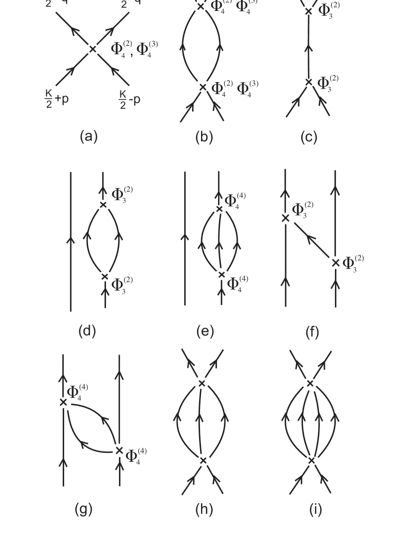
Figure 8: Perturbation diagrams contributing to the 2-particle scattering amplitude.

At leading order in $\lambda$, we find

$$M^{S}(K,q,p)\sim\lambda[\cos(K/2)(\cos p+\cos q)-\cos p\cos q]$$ (59)

and

$$M^{T}(K,q,p)\sim-\frac{\lambda}{2}\sin p\sin q$$ (60)

Following Shevchenko et al. shevchenko1999a , one can then find simple solutions (unnormalized) to the Schrödinger equation (51):

$$\psi^{S}(K,q) \sim \frac{\cos(K/2)-\cos q}{1+\cos^{2}(K/2)-2\cos(K/2)\cos q},$$

$$\psi^{T}(K,q) \sim \frac{\sin q}{1+4\cos^{2}(K/2)-4\cos(K/2)\cos q},$$ (61)

corresponding to bound-state energies

$$E^{S}(K) \sim 2-\frac{\lambda}{2}(1+\cos^{2}(K/2))$$

$$E^{T}(K) \sim 2-\frac{\lambda}{4}(1+4\cos^{2}(K/2))$$ (62)

compared to the lower edge of the 2-particle continuum

$$E_{2}(K)\sim 2-\lambda\cos(K/2).$$ (63)

These agree with the dimer series expansion barnes1999 ; trebst2000 at leading order.

Note, however, that the singlet solution is valid for all $K$, touching the continuum at $K=0$; while the triplet solution is only physically valid over a finite range of momenta $K=\{2\pi/3,4\pi/3\}$, and not at $K=0$. The end-points of this range are just where the triplet bound state enters the continuum, and the denominator of (61) for $\psi^{T}$ vanishes at $q=0$. Note also that both dispersion curves meet the lower edge of the continuum at a tangent.

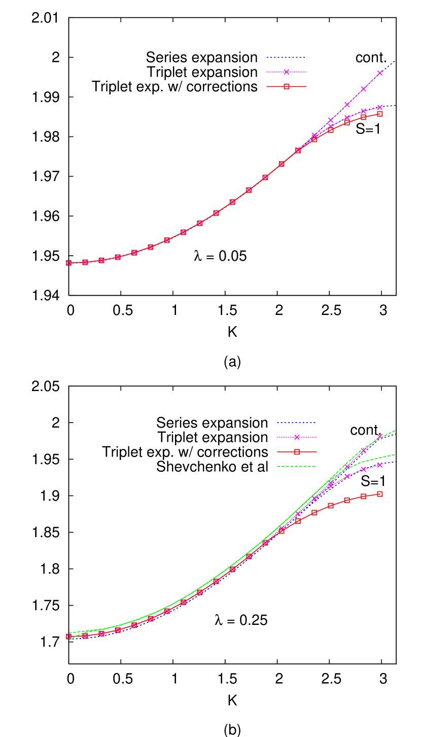
Figure 9: Dispersion relation for the triplet ($S=1$) 2-particle bound state at selected couplings a) $\lambda=0.05$ and b) $\lambda=0.25$. The lower edge of the continuum is labelled ’cont’.

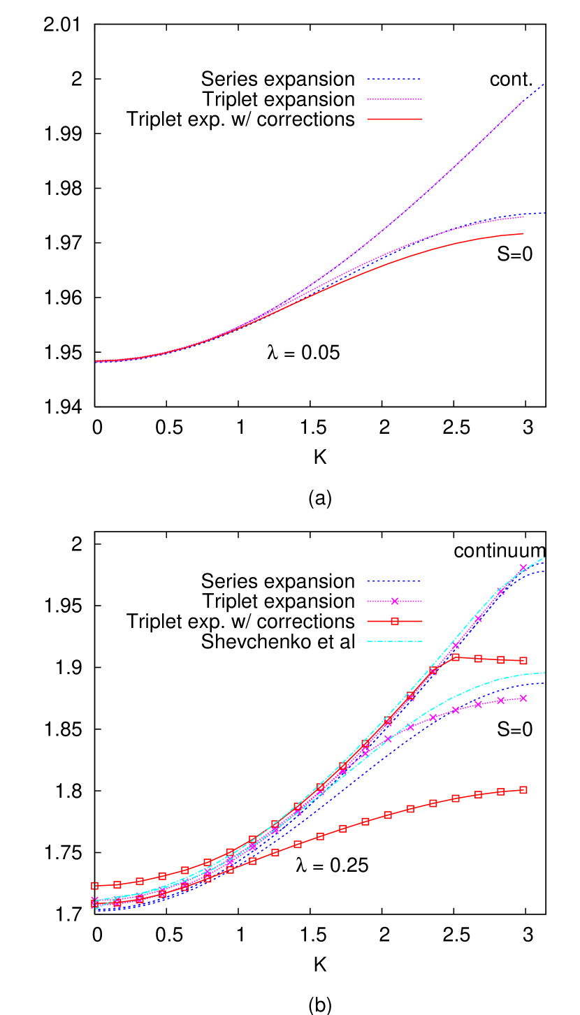
Figure 10: [Color online] Dispersion relation for singlet ($S=0$) 2-particle bound states at selected couplings a) $\lambda=0.05$ and b) $\lambda=0.25$. The lower edge of the continuum is labelled ’cont’.

At the next order O($\lambda^{2}$), further diagrams contribute, as given in Figures 8b)-i). Two of these, Figures 8h) and 8i), we are not in a position to calculate, because they involve 5 or 6-particle vertices. Figure 8b) is already accounted for by diagonalizing the effective Hamiltonian in the 2-particle subspace. Diagrams 8d) and 8e) simply correspond to renormalizations of the single-particle energies in the diagonal terms of the effective Hamiltonian in the 2-body sector. Finally, we can calculate the contribution of Figures 8c), 8f) and 8g) to the effective Hamiltonian using perturbation theory. In general, the change in the energy eigenvalue is

$$\Delta E=\frac{1}{N}\sum_{p,q}\Delta M(K,q,p)\psi(K,p)\psi(K,q)$$ (64)

where the vertex function $\Delta M(K,q,p)$ for each different diagram and spin state is listed in Appendix B.

The corrections due to these diagrams can now be calculated. On a finite lattice, equation (51) becomes a matrix eigenvalue equation, which can readily be solved numerically. We have calculated results for lattices of up to $N=40$. The resulting bound-state spectrum is displayed in Figures 9 and 10. The first thing to note is that the modified but uncorrected triplet expansion agrees with series expansion estimates quite well, for both the lowest-lying singlet and triplet bound states. For the triplet state, the result is substantially better than that of Shevchenko et al. shevchenko1999a at $\lambda=0.25$. Inclusion of the perturbation corrections actually makes the agreement worse, and gives much too large binding energies, especially at $\lambda=0.25$. This can be attributed to the neglect of diagrams 8h),i), which are of the same order as the diagrams we have calculated. Unless the extra diagrams are included, we cannot do better than the uncorrected estimates.

We have also looked for signs of the second singlet and second triplet bound states which were found to appear at order $\lambda^{2}$ by Trebst et al. trebst2000 . In the corrected results, a second singlet bound state does appear, in fact, but with much too large a binding energy once again. The detailed dynamics of the bound states are sensitive to higher-order terms.

IV.4 Structure Factors

The “reduced exclusive structure factor” or spectral weight for a specific intermediate state $\Lambda$ with momentum ${\bf K}$ can be written

$$S^{\alpha\alpha}_{\Lambda}(K)=|\Omega_{\Lambda}^{\alpha}(K)|^{2}$$ (65)

where

$$\Omega_{\Lambda}^{\alpha}(K)=\sqrt{N}\sum_{i^{*}}<\Psi_{\Lambda}(K)|S^{\alpha}_{i^{*}}|\Psi_{0}>\exp(-iK\cdot r_{i^{*}})$$ (66)

and the sum $i^{*}$ runs over sites of the unit cell on the lattice, and N is the number of unit cells (dimers). Using equations (9), (15), and (17), the spin operators $S_{1}$ and $S_{2}$ on sites 1 and 2 can be expressed in terms of triplet operators (taking $n=0$ in equation (15)):

$$S_{1,2}^{\alpha} = \pm\sum_{k}T_{1}^{(1)}(k)(\tau_{k\alpha}+\tau^{\dagger}_{k\alpha})-i\epsilon_{\alpha\beta\gamma}\sum_{12}[T_{2}^{(1)}(12)(\tau_{1\beta}^{\dagger}\tau_{2\gamma}^{\dagger}-\tau_{2\beta}^{\dagger}\tau_{1\gamma}^{\dagger}+\tau_{2\beta}\tau_{1\gamma}-\tau_{1\beta}\tau_{2\gamma})$$ (67)

$$+T_{2}^{(2)}(12)(\tau_{1\beta}^{\dagger}\tau_{2\gamma}+\tau_{2\beta}^{\dagger}\tau_{1\gamma}-\tau_{2\gamma}^{\dagger}\tau_{1\beta}-\tau_{1\gamma}^{\dagger}\tau_{2\beta})]$$

$$\mp\sum_{123}\left[T_{3}^{(1)}(123)(\tau^{\dagger}_{1\alpha}\tau^{\dagger}_{2\gamma}\tau^{\dagger}_{3\gamma}+\tau^{\dagger}_{2\gamma}\tau^{\dagger}_{3\gamma}\tau_{1\alpha}+\tau^{\dagger}_{1\alpha}\tau_{2\gamma}\tau_{3\gamma}+\tau_{2\gamma}\tau_{3\gamma}\tau_{1\alpha})+T_{3}^{(2)}(123)(\tau^{\dagger}_{1\alpha}\tau^{\dagger}_{2\gamma}\tau_{3\gamma}+\tau^{\dagger}_{3\gamma}\tau_{2\gamma}\tau_{1\alpha})\right]$$

where the upper and lower signs correspond to $S_{1}^{\alpha},S_{2}^{\alpha}$ respectively, and

$$T_{1}^{(1)}(k)=\frac{1}{2\sqrt{N}}(c_{k}+s_{k})(1-R_{1}-4R_{2})$$ (68)

$$T_{2}^{(1)}(12)=\frac{1}{8N}(c_{1}s_{2}-s_{1}c_{2})$$ (69)

$$T_{2}^{(2)}(12)=\frac{1}{8N}(c_{1}c_{2}-s_{1}s_{2})$$ (70)

$$T_{3}^{(1)}(123)=\frac{(c_{1}+s_{1})}{4N^{3/2}}(c_{2}s_{3}+s_{2}c_{3})$$ (71)

and

$$T_{3}^{(2)}(123)=\frac{(c_{1}+s_{1})}{2N^{3/2}}(c_{2}c_{3}+s_{2}s_{3})$$ (72)

In leading order (Figure 11a), the one-particle matrix element is

$$\Omega_{\Lambda}^{\alpha}(K) = i\sin(\frac{Ka}{2})[(1-R_{1}-4R_{2})(c_{K}+s_{K})]$$ (73)

$$\sim i\sin(\frac{Ka}{2})[1+\frac{\lambda}{4}\cos K$$

$$+\frac{\lambda^{2}}{64}(5\cos 2K-7)].$$

Here $a$ represents the spacing between spins in the dimer, i.e. $a=1/2$ for the uniform lattice in our present units.

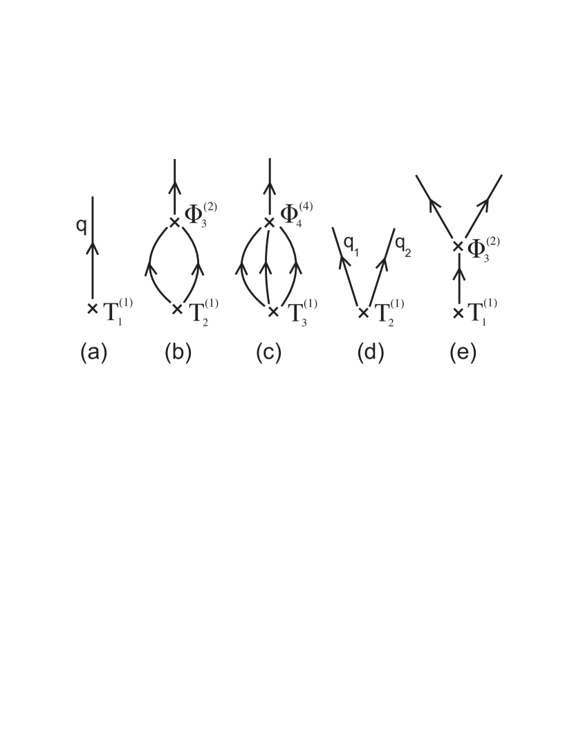
Figure 11: Perturbation diagrams contributing to exclusive structure factors.

Higher-order diagrams such as Figs. 11b), c) do not contribute until O($\lambda^{2}$). Their contributions are listed in Appendix C. Hence we find

$$\Omega_{1p}^{\alpha(11b)}\sim i\cos(\frac{Ka}{2})\frac{\lambda^{2}}{8}\sin K$$ (74)

$$\Omega_{1p}^{\alpha(11c)}\sim i\sin(\frac{Ka}{2})\frac{\lambda^{2}}{8}.$$ (75)

We must also account for the renormalization of the 1-particle wave function due to Figures 3a) and 3b), giving a multiplicative renormalization factor

$$Z_{K} = 1-\frac{\lambda^{2}}{2N}\sum_{12}\delta_{1+2-K}\left[\frac{\Phi_{3}^{(2)}(12k)}{E_{K}-E_{1}-E_{2}}\right]^{2}-\frac{\lambda^{2}}{16N^{2}}\sum_{123}\delta_{1+2+3-K}\frac{\Phi_{4}^{(4)}(123K)}{(E_{K}-E_{1}-E_{2}-E_{3})^{2}}[3\Phi_{4}^{(4)}(123K)$$ (76)

$$+\Phi_{4}^{(4)}(321K)+\Phi_{4}^{(4)}(312K)]$$

$$\sim 1-\frac{\lambda^{2}}{8}\cos K-\frac{3\lambda^{2}}{16}$$

giving a total amplitude

$$\Omega_{1p}^{\alpha}(K) \sim i[\sin(\frac{Ka}{2})[1+\frac{\lambda}{4}\cos K+\frac{\lambda^{2}}{64}(-11-8\cos K+5\cos 2K)]+\cos(\frac{Ka}{2})\frac{\lambda^{2}}{8}\sin K]$$ (77)

whereas Zheng et al. zheng2003 obtain

$$\Omega_{1p}^{\alpha}(K) \sim i[\sin(\frac{Ka}{2})[1+\frac{\lambda}{4}\cos K+\frac{\lambda^{2}}{6}(-11-4\cos K+5\cos 2K)]+\cos(\frac{Ka}{2})\frac{\lambda^{2}}{8}\sin K]$$ (78)

We have been unable to resolve the source of the discrepancy at order $\lambda^{2}$.

The calculated results for the one-particle spectral weight are displayed in Figure 12. It can be seen that the results match the series estimates quite well, even at larger $\lambda$. The corrected estimates are a little low at small $k$, and a little high at large $k$: this reflects the discrepancy at order $\lambda^{2}$ referred to above.

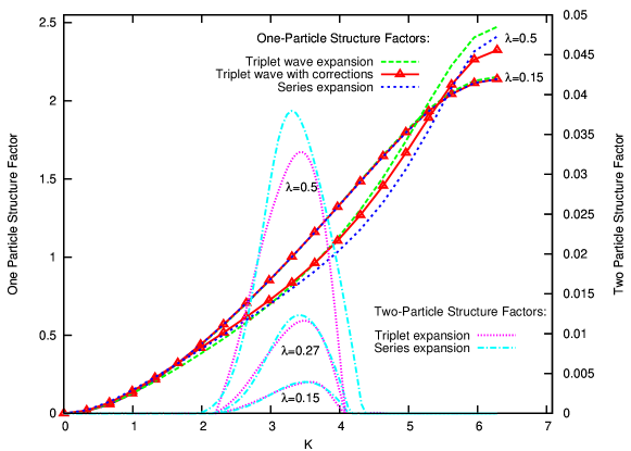
Figure 12: [Color online] The 1-particle (left axis) and 2-particle (right axis) spectral weights as functions of momentum at selected couplings $\lambda$.

For the 2-particle bound states, the leading perturbation diagrams contributing to the exclusive structure factors are illustrated in Figs. 11d),e). Their contributions for the triplet states are

$$\Omega_{T}^{\alpha[11d]}(K) = -8i\sqrt{N}\cos(\frac{Ka}{2})\times$$ (79)

$$\sum_{q}\psi^{T}(K,q)T_{2}^{(1)}(K/2+q,K/2-q)$$

$$\sim -i\frac{\lambda}{2\sqrt{N}}\cos(\frac{Ka}{2})\sin(K/2)$$

$$\times\sum_{q}\sin q\psi^{T}(K,q)$$

and

$$\Omega_{T}^{\alpha[11e]}(K) = 2i\lambda\sin(\frac{Ka}{2})T_{1}^{(1)}(K)\times$$ (80)

$$\sum_{q}\psi^{T}(K,q)\frac{\Phi_{3}^{(2)}(K/2+q,K/2-q,K)}{E_{K/2+q}+E_{K/2-q}-E_{K}}$$

$$\sim i\frac{\lambda}{\sqrt{N}}\sin(\frac{Ka}{2})\cos(K/2)$$

$$\times\sum_{q}\sin q\psi^{T}(K,q)$$

Inserting the wave function 61, we obtain the leading order behaviour of the triplet bound state contribution to the structure factor (for the uniform case $a=1/2$):

$$S_{T}^{\alpha\alpha}(K)\sim\frac{\lambda^{2}}{2}\sin^{6}(K/4)(1-4\cos^{2}(K/2)),$$ (81)

which agrees with the leading order series calculation zheng2003 . Thus the bound-state spectral weight vanishes at the threshold points $\{\cos(K/2)=\pm 1/2\}$ where the bound state merges with the continuum.

The numerically calculated results for the spectral weights are displayed in Figure 12. For the 1-particle weight, it can be seen that the corrected triplet-wave expansion matches the series estimates very well at the two lower couplings, and only begins to deviate significantly at $\lambda=0.5$. The triplet wave expansion also works surprisingly well for the 2-particle weight, which is only of order $1\%$ of the 1-particle weight.

V Summary and Conclusions

In this paper, we have developed a modified triplet-wave expansion method for dimerized spin systems, analogous to the modified spin-wave formalism takahashi1987 ; gochev1994 for magnetically ordered systems. It differs from the earlier approaches of Sachdev and Bhatt sachdev1990 and Kotov et al. kotov1998 in that projection operators are used to confine the system to the physical subspace in the bosonic formulation, eliminating the need for a separate constraint. The two-body boson operators are also fully diagonalized through the highest order calculated.

The formalism has been applied to the case of the alternating Heisenberg spin chain. Using perturbation theory to second order, we have calculated the ground-state energy per dimer, the dispersion relations for one-particle states and two-particle bound states, and the spectral weights for these states. It has been shown that the results reproduce the leading order terms in a dimer series expansion in powers of $\lambda$ singh1999 ; trebst2000 ; zheng2003 , apart from an unexplained discrepancy at order $\lambda^{2}$ in the 1-particle spectral weight. The results are quantitatively accurate at small $\lambda$, but begin to show significant discrepancies from high-order series expansions at larger $\lambda$, as one would expect. The discrepancies become more serious for the more sensitive dynamical quantities such as two-particle binding energies. The inclusion of a partial set of higher-order corrections for the two-particle binding energies made things worse rather than better, as one perhaps should have expected: all terms of a similar order in $\lambda$ must be included simultaneously if a good result is to be obtained. Nevertheless, the qualitative behaviour is correctly reproduced by the formalism. In particular, the formation of two-triplon bound states near $K=\pi/2$ in both the singlet ($S=0$) and triplet ($S=1$) channels, which was discovered previously uhrig1996 ; shevchenko1999a is reproduced.

The behaviour of the triplet bound state near the threshold where it merges with the continuum is interesting. We have seen that the bound-state dispersion curve merges at a tangent to the continuum, and that the spectral weight vanishes at the threshold. The bound-state solution does not extend into the continuum, but terminates at the threshold. This provides a neat example of the phenomenon of “quasiparticle breakdown” discussed recently in the literature masuda2006 ; stone2006 ; zhitomirsky2006 : i.e. the termination of a single-particle state where it enters the continuum for one-dimensional systems.

Our results appear to be more accurate and reliable at intermediate couplings $\lambda$ than those of Shevchenko et al. shevchenko1999a . However, they cannot match the quantitative accuracy of the high-order dimer series expansions singh1999 ; trebst2000 ; zheng2003 or exact diagonalization on large lattices barnes1999 . The calculations could be pushed to higher orders with the aid of a computer, but it is doubtful whether this is worthwhile. The main value of a ‘lattice bosonization’ approach such as this is to provide a better analytic understanding of the behaviour of the model, and a half-way house towards a continuum ‘effective field theory’ for the model. For instance, we have shown how the triplon mass parameter and the ‘speed of light’ can be calculated, which would be fundamental parameters of the effective field theory. It would be interesting to apply the approach to dimerized models in two dimensions.

$$\Phi^{(1)}_{3}(123) = \frac{1}{6}[\sin k_{1}(c_{1}+s_{1})(c_{2}s_{3}-s_{2}c_{3})+\sin k_{2}(c_{2}+s_{2})(c_{3}s_{1}-s_{3}c_{1})$$ (82)

$$+\sin k_{3}(c_{3}+s_{3})(c_{1}s_{2}-s_{1}c_{2})]$$

$$\Phi^{(2)}_{3}(123) = \frac{1}{2}[\sin k_{1}(c_{1}+s_{1})(c_{2}c_{3}-s_{2}s_{3})+\sin k_{2}(c_{2}+s_{2})(s_{1}s_{3}-c_{1}c_{3})+\sin k_{3}(c_{3}+s_{3})(s_{1}c_{2}-c_{1}s_{2})]$$ (83)

$$\Phi^{(1)}_{4}(1234) = \frac{1}{4}[(\cos k_{1}+\cos k_{2})(c_{1}c_{2}+c_{1}s_{2}+s_{1}c_{2}+s_{1}s_{2})(c_{3}s_{4}+s_{3}c_{4})$$ (84)

$$+(\cos k_{3}+\cos k_{4})(c_{3}c_{4}+c_{3}s_{4}+s_{3}c_{4}+s_{3}s_{4})(c_{1}s_{2}+s_{1}c_{2})$$

$$+\cos(k_{1}+k_{4}))(c_{1}s_{4}-s_{1}c_{4})(s_{2}c_{3}-c_{2}s_{3})$$

$$+\cos(k_{1}+k_{3})(c_{1}s_{3}-s_{1}c_{3})(s_{2}c_{4}-c_{2}s_{4})]$$

$$\Phi^{(2)}_{4}(1234) = \frac{1}{2}[(\cos k_{1}+\cos k_{2})(c_{1}c_{2}+c_{1}s_{2}+s_{1}c_{2}+s_{1}s_{2})(s_{3}c_{4}+c_{3}s_{4})$$ (85)

$$+(\cos k_{4}+\cos k_{3})(c_{1}s_{2}+s_{1}c_{2})(c_{3}c_{4}+c_{3}s_{4}+s_{3}c_{4}+s_{3}s_{4})$$

$$+\cos(k_{1}-k_{3})(s_{1}c_{2}s_{3}c_{4}+c_{1}s_{2}c_{3}s_{4}-c_{1}c_{2}c_{3}c_{4}-s_{1}s_{2}s_{3}s_{4})$$

$$+\cos(k_{1}-k_{4})(c_{1}s_{2}s_{3}c_{4}+s_{1}c_{2}c_{3}s_{4}-c_{1}c_{2}c_{3}c_{4}-s_{1}s_{2}s_{3}s_{4})]$$

$$\Phi^{(3)}_{4}(1234) = \cos k_{1}((c_{1}c_{2}+s_{1}c_{2})(s_{3}c_{4}+c_{3}c_{4})+(c_{1}s_{2}+s_{1}s_{2})(s_{3}s_{4}+c_{3}s_{4}))+\cos k_{2}((c_{1}c_{2}+c_{1}s_{2})(c_{3}s_{4}+c_{3}c_{4})$$ (86)

$$+(s_{1}c_{2}+s_{1}s_{2})(s_{3}s_{4}+s_{3}c_{4}))+\cos k_{3}((c_{1}s_{2}+s_{1}s_{2})(c_{3}s_{4}+s_{3}s_{4})+(s_{1}c_{2}+c_{1}c_{2})(s_{3}c_{4}+c_{3}c_{4}))$$

$$+\cos k_{4}((s_{1}c_{2}+s_{1}s_{2})(s_{3}c_{4}+s_{3}s_{4})+(c_{1}s_{2}+c_{1}c_{2})(c_{3}s_{4}+c_{3}c_{4}))$$

$$+\cos(k_{1}-k_{4})(c_{1}c_{4}-s_{1}s_{4})(c_{2}c_{3}-s_{2}s_{3})$$

$$+\cos(k_{1}+k_{2})(c_{1}s_{2}-s_{1}c_{2})(c_{3}s_{4}-s_{3}c_{4})$$

$$\Phi^{(4)}_{4}(1234) = (\cos k_{1}+\cos k_{2})(c_{1}c_{2}+s_{1}s_{2}+c_{1}s_{2}+s_{1}c_{2})(c_{3}c_{4}+s_{3}s_{4})+(\cos k_{3}+\cos k_{4})(c_{1}s_{2}+s_{1}c_{2})(c_{3}s_{4}$$ (87)

$$+s_{3}c_{4}+c_{3}c_{4}+s_{3}s_{4})+\cos(k_{2}+k_{3})(c_{1}s_{2}c_{3}c_{4}+s_{1}c_{2}s_{3}s_{4}-c_{1}c_{2}s_{3}c_{4}-s_{1}s_{2}c_{3}s_{4})$$

$$+\cos(k_{1}+k_{3})(s_{1}c_{2}c_{3}c_{4}+c_{1}s_{2}s_{3}s_{4}-c_{1}c_{2}s_{3}c_{4}-s_{1}s_{2}c_{3}s_{4})$$

We have ‘symmetrized’ these expressions with respect to their indices, using momentum conservation.

APPENDIX B

The two-body terms $\Delta M(K,p,q)$ defined in equation (54) for the diagrams Figs. 8c), f) and g) are as follows (the energy denominators are ‘symmetrized’ between initial and final states):

Scalar state

$$\Delta M_{S}^{(9c)}(K,q,p)=0$$ (88)

$$\Delta M_{S}^{(9f)}(K,q,p) = \lambda^{2}\left\{\frac{\Phi_{3}^{(2)}(p-q,K/2+q,K/2+p)\Phi_{3}^{(2)}(K/2-p,p-q,K/2-q)}{(E_{p-q}+1/2(E_{K/2+q}+E_{K/2-p}-E_{K/2+p}-E_{K/2-q}))}\right.$$ (89)

$$\left.+(ditto,p\rightarrow-p)+(ditto,q\rightarrow-q)+(ditto,p\leftrightarrow-p,q\leftrightarrow-q)\right\}$$

$$\Delta M_{S}^{(9g)}(K,q,p) = -\frac{\lambda^{2}}{16N}\sum_{k}\left\{[\Phi_{4}^{(4)}(p-q-k,k,K/2+q,K/2+p)(3\Phi_{4}^{(4)}(k,p-q-k,K/2-p,K/2-q)\right.$$ (90)

$$+\Phi_{4}^{(4)}(K/2-p,k,p-q-k,K/2-q)+\Phi_{4}^{(4)}(K/2-p,p-q-k,k,K/2-q))$$

$$+2\Phi_{4}^{(4)}(K/2+q,p-q-k,k,K/2+p)\times(3\Phi_{4}^{(4)}(K/2-p,k,p-q-k,K/2-q)$$

$$+\Phi_{4}^{(4)}(k,p-q-k,K/2-p,K/2-q)+\Phi_{4}^{(4)}(K/2-p,p-q-k,k,K/2-q))]$$

$$/(E_{k}+E_{p-q-k}+1/2(E_{K/2+q}+E_{K/2-p}-E_{K/2+p}-E_{K/2-q}))$$

$$+(ditto,p\leftrightarrow-p)+(ditto,q\leftrightarrow-q)+(ditto,p\leftrightarrow-p,q\leftrightarrow-q)\large\}$$

Triplet state

$$\Delta M_{T}^{(9c)}(K,q,p)=\lambda^{2}\frac{\Phi_{3}^{(2)}(K/2+p,K/2-p,K)\Phi_{3}^{(2)}(K/2+q,K/2-q,K)}{(E_{K}-1/2(E_{K/2+q}+E_{K/2-q}+E_{K/2+p}+E_{K/2-p}))}$$ (91)

$$\Delta M_{T}^{(9f)}(K,q,p) = \frac{\lambda^{2}}{2}\left\{\frac{\Phi_{3}^{(2)}(p-q,K/2+q,K/2+p)\Phi_{3}^{(2)}(K/2-p,p-q,K/2-q)}{(E_{p-q}+1/2(E_{K/2+q}+E_{K/2-p}-E_{K/2+p}-E_{K/2-q}))}\right.$$ (92)

$$\left.-(ditto,p\leftrightarrow-p)-(ditto,q\leftrightarrow-q)+(ditto,p\leftrightarrow-p,q\leftrightarrow-q)\right\}$$

$$\Delta M_{T}^{(9g)}(K,q,p) = -\frac{\lambda^{2}}{16N}\sum_{k}\left\{[\Phi_{4}^{(4)}(p-q-k,k,K/2+q,K/2+p)(3\Phi_{4}^{(4)}(k,p-q-k,K/2-p,K/2-q)\right.$$ (93)

$$+\Phi_{4}^{(4)}(k,K/2-p,p-q-k,K/2-q)+\Phi_{4}^{(4)}(p-q-k,K/2-p,k,K/2-q))$$

$$+2\Phi_{4}^{(4)}(p-q-k,K/2+q,k,K/2+p)\times(\Phi_{4}^{(4)}(k,p-q-k,K/2-p,K/2-q)$$

$$-\Phi_{4}^{(4)}(p-q-k,K/2-p,k,K/2-q))]$$

$$/(E_{k}+E_{p-q-k}+1/2(E_{K/2+q}+E_{K/2-p}-E_{K/2+p}-E_{K/2-q}))$$

$$\left.-(ditto,p\leftrightarrow-p)-(ditto,q\leftrightarrow-q)+(ditto,p\leftrightarrow-p,q\leftrightarrow-q)\right\}$$

APPENDIX C

Contributions to the 1-particle matrix elements $\Omega_{\Lambda}^{\alpha}(K)$ from the diagrams shown in Figure 11b),c) are:

$$\Omega_{1p}^{\alpha[11b]}(K) = 4i\lambda\cos(\frac{Ka}{2})\sum_{12}\delta_{1+2-K}\frac{T_{2}^{(1)}(12)}{E_{K}-E_{1}-E_{2}}[\Phi_{3}^{(2)}(21K)-\Phi_{3}^{(2)}(12K)]$$ (94)

$$\Omega_{1p}^{\alpha[11c]}(K) = -i\frac{\lambda}{\sqrt{N}}\sin(\frac{Ka}{2})\sum_{123}\delta_{1+2+3-K}\frac{T_{3}^{(1)}(123)}{E_{K}-E_{1}-E_{2}-E_{3}}[3\Phi_{4}^{(4)}(321K)+\Phi_{4}^{(4)}(312K)+\Phi_{4}^{(4)}(213K)]$$ (95)

References

- (1) B.S. Shastry and B. Sutherland, Physica 108B, 1069 (1981).
- (2) For a review, see C. Lhuillier and G. Misguich, cond-mat/0109146, Lecture Notes at the Cargèse Summer School on Trends in high magnetic field science (May 2001).
- (3) N. Read and S. Sachdev, Phys. Rev. Lett. 66, 1773 (1991); ibid 62, 1694 (1989); G. Murthy and S. Sachdev, Nucl. Phys. B344, 557 (1990).
- (4) V.N. Kotov, J. Oitmaa, O.P. Sushkov and Zheng W-H., Phys. Rev. B 60, 14613 (1999); O.P. Sushkov, J. Oitmaa and W-H. Zheng, Phys. Rev. B63, 104420 (2001).
- (5) P.W. Anderson, Science 235, 1196 (1987).
- (6) L. Capriotti and S. Sorella, Phys. Rev. Lett. 84, 3173 (2000); L. Capriotti, F. Becca, A. Parola and S. Sorella, Phys. Rev. B67, 212402 (2003).
- (7) S. Sachdev and R. Bhatt, Phys. Rev. B41, 9323 (1990).
- (8) A.V. Chubukov, JETP Lett. 49, 129 (1989).
- (9) D.C. Mattis, The Theory of Magnetism, Vol. II, Vol. 55 of Springer Series in Solid-State Sciences (Springer-Verlag, Berlin, 1981).
- (10) V.N. Kotov, Zheng W-H, O.P. Sushkov and J. Oitmaa, Phys. Rev. Letts. 80, 5790 (1998).
- (11) P.V. Shevchenko and O.P. Sushkov, Phys. Rev. B59, 8383 (1999).
- (12) O.P. Sushkov and V.N. Kotov, Phys. Rev. Letts. 81, 1941 (1998).
- (13) V.N. Kotov, O.P. Sushkov and R. Eder, Phys. Rev. B59, 6266 (1999).
- (14) P.V. Shevchenko and O.P. Sushkov, Phys. Rev. B59, 8383 (1999).
- (15) M. Takahashi, Phys. Rev. Lett. 58, 168 (1987); Phys. Rev. B40, 2494 (1989).
- (16) I. G. Gochev, Phys. Rev. B49, 9594 (1994).
- (17) G. Xu, C. Broholm, D.H. Reich and M.A. Adams, Phys. Rev. Lett. 84, 4465 (2000).
- (18) D.A. Tennant, C. Broholm, D.H. Reich, S.E. Nagler, G.E. Granroth, T. Barnes, K. Damle, G. Xu, Y. Chen and B.C. Sales, Phys. Rev. B67, 054414 (2003).
- (19) T. Barnes, J. Riera and D.A. Tennant, Phys. Rev. B59, 11384 (1999).
- (20) G.S. Uhrig and H.J. Schulz, Phys. Rev. B54, R9624 (1996).
- (21) A. Fledderjohann and C. Gros, Europhys. Lett. 37, 189 (1997).
- (22) G. Bouzerar, A.P. Kampf and G.I. Japaridze, Phys. Rev. B58, 3117 (1998)
- (23) G. Bouzerar and S. Sil, Int. J. Mod. Phys. 15, 2821 (2001).
- (24) R.R.P. Singh and Zheng W-H., Phys. Rev. B59, 9911 (1999).
- (25) S.Trebst, H. Monien, C.J. Hamer, W-H Zheng and R.R.P. Singh, Phys. Rev. Let.t 85, 4373 (2000); W-H Zheng, C.J. Hamer, R.R.P. Singh, S. Trebst and H. Monien, Phys. Rev. B63, 144411 (2001).
- (26) W-H. Zheng, C.J. Hamer and R.R.P. Singh, Phys. Rev. Lett. 91, 037206 (2003); C.J. Hamer, W-H. Zheng and R.R.P. Singh, Phys. Rev. B68, 214408 (2003).
- (27) J.D. Johnson, S. Krinsky and B.M. McCoy, Phys. Rev. A8, 2526 (1973).
- (28) T. Masuda, A. Zheludev, H. Manaka, L-P. Regnault, J-H. Chung and Y. Qiu, Phys. Rev. Letts. 96, 047210 (2006).
- (29) M.B. Stone, I.A. Zalisnyak, T. Hong, C.L. Broholm and D.H. Reich, Nature 440, 187 (2006).
- (30) M.E. Zhitomirsky, Phys. Rev. B73, 100404R (2006).