Two-phonon spin-lattice relaxation of rigid atomic clusters

Abstract

Spin-phonon relaxation due to two-phonon processes of a spin cluster embedded in an elastic medium has been studied. For the case of uniaxial anisotropy, relaxation rates due to Raman processes and processes involving the emission of two phonons have been obtained. For a biaxial spin Hamiltonian, the rates of transitions between tunnel-split levels have been computed. By comparison with the rates of corresponding direct processes, we have established temperature ranges where the Raman mechanism dominates over the one-phonon decay mechanism.

I Introduction

Relaxation of spins in a paramagnetic solid is a problem of fundamental interest. It is also related to important applications such as spin resonance and the use of spin as a qubit. In a paramagnet, the decay of a spin state is due to the interactions with phonons, nuclear spins, dipolar fields, etc. In principle, one could suppress the interaction with nuclear spins and dipolar fields but the interaction with phonons always remains. Often it dominates spin relaxation. Thus, spin-lattice interactions provide the most fundamental upper bound for the lifetime of spin states in paramagnets. The spin relaxation due to interaction with the lattice can occur by various mechanisms. The most studied and often the dominant ones are direct processes, in which a single quantum is exchanged between the spin system and the lattice. It was pointed out by Waller in studying the modulation of the spin-spin interaction by the lattice waves that, unlike in electromagnetic phenomena, the inelastic scattering of a phonon combined with a transition in the spin system could be very important Waller . This is a two-phonon process consisting of the absorption of one phonon and the emission of another phonon with different frequency. The mechanism is analogous to the Raman effect in optical spectroscopy and it is often referred to as a Raman process. Spin-lattice relaxation mechanisms based on dipolar interactions (Waller) were insufficient, however, to account for the transition rates measured in experiment. Heitler and Teller Heitler considered Raman processes based on a more potent mechanism based upon modulation of the crystal electric field under the action of the lattice vibrations. Their theory was further developed by Kronig Kronig and Van Vleck VanVleck . They obtained a spin-phonon coupling based on the spin-orbit interaction that permitted calculation of relaxation rates that were of the same order of magnitude as the experimental ones. Later on, Orbach Orbach managed to simplify the treatment of the problem by expanding the crystal electric potential in powers of the fluctuating strain caused by the lattice vibrations.

Recently, this problem has received new attention in connection with spin relaxation of molecular clusters. The spin of many such clusters is formed inside a relatively rigid magnetic core that can rotate in the presence of the deformation field but is more resistant to distortions of the core itself. It has been noticed that the spin relaxation of such a cluster can be obtained within a model that is parameter free, that is, it gives the relaxation rates in terms of the known crystal field Hamiltonian of the magnetic core $\hat{\cal{H}}_{A}$ CGS . Even for non-rigid clusters, calculation of the effect of rotations is meaningful. It has been theoretically established that spin-phonon relaxation rates due to both, one-phonon and multi-phonon processes, are inversely proportional to some high powers of the sound velocity A&B . Since longitudinal phonons have a larger sound velocity than the transverse phonons, processes involving longitudinal phonons can be safely neglected. The effects of the transverse phonons can be split into shear deformations of the lattice cell and local rotations of the lattice that preserve the symmetry of the crystal field. To describe deformations of the first kind one needs to employ terms in the Hamiltonian containing phenomenological coupling constants, whereas the local rotations can be described by a parameter-free spin-phonon Hamiltonian that is defined solely by the form of $\hat{\cal{H}}_{A}$. In general, processes due to the shear distortion of the lattice and those due to the local rotation of the lattice should result in comparable relaxation rates. Even in this case, the latter are of a fundamental importance because they provide a parameter-free lower bound on the decoherence of any spin-based qubit. For rigid spin clusters, interaction of the spin with rotations of the crystal field is the only source of spin-lattice relaxation.

The angle of rotation of the crystal field axes $({\mathbf{e}}^{(1)},{\mathbf{e}}^{(2)},{\mathbf{e}}^{(3)})$ due to the action of the phonon field ${\mathbf{u}}({\mathbf{r}})$ is given by

$$\delta{\mathbf{\phi}}({\mathbf{r}})=\frac{1}{2}\nabla\times{\mathbf{u}}({\mathbf{r}}).$$ (1)

Because $\mathcal{\hat{H}}_{A}$ is a scalar, the rotation of $({\mathbf{e}}^{(1)},{\mathbf{e}}^{(2)},{\mathbf{e}}^{(3)})$ is equivalent to the rotation of the vector ${\mathbf{S}}$ in the opposite direction. As it is known, the rotation of the operator ${\mathbf{S}}$ can be performed by the $(2S+1)\times(2S+1)$ matrix in the spin space,

$${\mathbf{S}}\rightarrow\hat{R}{\mathbf{S}}\hat{R}^{-1},\qquad\hat{R}=e^{-i{\mathbf{S}}\cdot\delta{\mathbf{\phi}}}\,.$$ (2)

Then, the total Hamiltonian in the presence of phonons can be written in the form CGS

$${\mathcal{\hat{H}}}=\hat{R}{\mathcal{\hat{H}}}_{A}\hat{R}^{-1}+{\mathcal{\hat{H}}}_{Z}+{\mathcal{\hat{H}}}_{ph}\,,$$ (3)

where ${\mathcal{\hat{H}}}_{A}$ is the crystal-field Hamiltonian in the absence of phonons, ${\mathcal{\hat{H}}}_{Z}$ is the Zeeman Hamitonian and ${\mathcal{\hat{H}}}_{ph}$ is the Hamiltonian of harmonic phonons. In these formulas $\delta{\bm{\phi}}$ must be treated as an operator. The canonical quantization of phonons and Eq. (1) yield

$$\delta\bm{\phi}=\sqrt{\frac{\hbar}{8\rho V}}\sum_{\mathbf{k}\lambda}\frac{\left[i\mathbf{k}\times\mathbf{e}_{\mathbf{k}\lambda}\right]e^{i\mathbf{k\cdot r}}}{\sqrt{\omega_{\mathbf{k}\lambda}}}\left(a_{\mathbf{k}\lambda}+a_{-\mathbf{k}\lambda}^{\dagger}\right)$$ (4)

where $\rho$ is the mass density, $V$ is the volume of the crystal, $\mathbf{e}_{\mathbf{k}\lambda}$ are unit polarization vectors, $\lambda=t_{1},t_{2},l$ denotes polarization, and $\omega_{k\lambda}=v_{\lambda}k$ is the phonon frequency.

For one-phonon processes, relaxation rates of spin-phonon transitions have been recently computed with the help of the above formalism in Ref. CGS, . Such processes dominate spin-phonon relaxation at zero temperature when no thermal phonons are present in the system. At finite temperature, however, two-phonon processes may take over. In this paper we study two kinds of two-phonon processes. The first kind consists of an inelastic scattering of phonons by the spin-system, or spin-phonon Raman processes. It corresponds to the annihilation of an incoming phonon of frequency $\omega_{\mathbf{k}}$ and the creation of an outgoing phonon of frequency $\omega_{\mathbf{q}}$, with ${\mathbf{k}}$ and ${\mathbf{q}}$ being the corresponding wave vectors. The second kind involves emission of two phonons. Note that the conservation of the energy in spin-phonon interactions requires

$$\hbar\omega_{\mathbf{q}}\pm\hbar\omega_{\mathbf{k}}=\Delta E>0\,,$$ (5)

where $\Delta E$ is the energy difference between the spin-states and $\omega_{\mathbf{k}},\omega_{\mathbf{q}}$ are the frequencies of the phonons involved in the transition. The plus sign applies to processes involving the emission of two phonons and the minus sign applies to Raman processes. When $\Delta E\ll\hbar\omega_{D}$ (with $\omega_{D}$ being the Debye frequency), Eq. (5) causes the phase space of phonons to be much greater for Raman processes than for processes involving the emission of two phonons. Consequently, the spin-phonon Raman scattering usually dominates over the processes involving the emission of two phonons. However, the same condition (5) implies that the energy of the phonon emitted in the Raman scattering process, $\hbar\omega_{\mathbf{q}}$, must satisfy $\hbar\omega_{\mathbf{q}}>\Delta E$, whereas in the process involving the creation of two phonons their energy must be smaller than $\Delta E$. Therefore, if $k_{B}T\ll\Delta E$, the total number of phonons available to carry out the spin transition may be much greater in the two-phonon emission case than in the Raman case, so that the former case can become dominant. In both cases the matrix element of the transition is a sum of two terms. The first term, $M^{(2)}$, comes from the first order of the perturbation theory on the spin-phonon coupling containing a product of two phonon displacement fields. The second term, $M^{(1+1)}$, comes from the second order of the perturbation theory on the spin-phonon coupling that is linear in the phonon displacement field. In some cases these two terms interfere, so that the resulting transition rate, based upon $|M^{(2)}+M^{(1+1)}|^{2}$, is different from the one obtained by adding up the rates, $|M^{(2)}|^{2}$ and $|M^{(1+1)}|^{2}$, that each term would produce by itself, as was incorrectly done in the past A&B .

II Matrix elements of two-phonon processes

The treatment of two-phonon processes requires consideration of terms up to second order in phonon amplitudes in the Hamiltonian:

$$\hat{R}{\mathcal{\hat{H}}}_{A}\hat{R}^{-1}\simeq{\mathcal{\hat{H}}}_{A}+{\mathcal{\hat{H}}}_{\mathrm{s-ph}}\qquad{\mathcal{\hat{H}}}_{\mathrm{s-ph}}={\mathcal{\hat{H}}}_{\mathrm{s-ph}}^{(1)}+{\mathcal{\hat{H}}}_{\mathrm{s-ph}}^{(2)}\,,$$ (6)

with

$${\mathcal{\hat{H}}}_{\mathrm{s-ph}}^{(1)} = i\left[{\mathcal{\hat{H}}}_{A},{S_{\alpha}}\right]\,\delta\phi_{\alpha}$$

$${\mathcal{\hat{H}}}_{\mathrm{s-ph}}^{(2)} = \frac{i^{2}}{2!}\left[\left[{\mathcal{\hat{H}}}_{A},S_{\alpha}\right],S_{\beta}\right]\delta\phi_{\alpha}\delta\phi_{\beta}\,.$$ (7)

The total Hamiltonian can then be written as

$${\mathcal{\hat{H}}}={\mathcal{\hat{H}}}_{0}+{\mathcal{\hat{H}}}_{\mathrm{s-ph}}\,,$$ (8)

where ${\mathcal{\hat{H}}}_{0}$ is the Hamiltonian of non-interacting spin and phonons,

$${\mathcal{\hat{H}}}_{0}={\mathcal{\hat{H}}}_{S}+{\mathcal{\hat{H}}}_{\mathrm{ph}}\,,$$ (9)

and

$${\mathcal{\hat{H}}}_{S}={\mathcal{\hat{H}}}_{A}+{\mathcal{\hat{H}}}_{Z}\,,$$ (10)

is the spin Hamiltonian.
We will study spin-phonon transitions between the eigenstates of ${\mathcal{\hat{H}}}_{0}$, which are direct products of the spin and phonon states,

$$\left|\Psi_{\pm}\right\rangle=\left|\psi_{\pm}\right\rangle\otimes\left|\phi_{\pm}\right\rangle.$$ (11)

Here $\left|\psi_{\pm}\right\rangle$ are the eigenstates of $\mathcal{\hat{H}}_{S}$ with eigenvalues $E_{\pm}$ ($E_{+}>E_{-}$) and $\left|\phi_{\pm}\right\rangle$ are the eigenstates of $\mathcal{\hat{H}}_{\mathrm{ph}}$ with energies $E_{\mathrm{ph},\pm}$. Spin-phonon transitions conserve energy

$$E_{+}+E_{\mathrm{ph},+}=E_{-}+E_{\mathrm{ph},-}.$$ (12)

To obtain the relaxation rate of the transition $\left|\Psi_{+}\right\rangle\rightarrow\left|\Psi_{-}\right\rangle$ one needs to evaluate the matrix element of the process. This matrix element is the sum of the matrix element with ${\mathcal{\hat{H}}}_{s-ph}^{(2)}$ and that with ${\mathcal{\hat{H}}}_{s-ph}^{(1)}$ in the second order Sakurai :

$$M=M^{(2)}+M^{(1+1)}\,,$$ (13)

where

$$M^{(2)}=\left\langle\Psi_{-}\left|{\mathcal{\hat{H}}}_{\mathrm{s-ph}}^{(2)}\right|\Psi_{+}\right\rangle$$ (14)

and

$$M^{(1+1)} = \sum_{\xi}\frac{\left\langle\Psi_{-}\left|{\mathcal{\hat{H}}}_{\mathrm{s-ph}}^{(1)}\right|\Psi_{\xi}\right\rangle\left\langle\Psi_{\xi}\left|{\mathcal{\hat{H}}}_{\mathrm{s-ph}}^{(1)}\right|\Psi_{+}\right\rangle}{E_{+}-E_{\xi}}.$$

Here $\xi$ labels intermediate spin-phonon states.

III Raman processes

For the Raman processes of interest, a phonon with the wave vector $\mathbf{k}$ is absorbed and a phonon with the wave vector $\mathbf{q}$ is emitted. We will use the following designations for the phonon states

$$\left|\phi_{+}\right\rangle\equiv\left|n_{\mathbf{k}},n_{\mathbf{q}}\right\rangle,\qquad\left|\phi_{-}\right\rangle\equiv\left|n_{\mathbf{k}}-1,n_{\mathbf{q}}+1\right\rangle$$ (16)

In this case, the conservation of the energy reads:

$$\Delta E=E_{+}-E_{-}=\hbar\omega_{\mathbf{q}}-\hbar\omega_{\mathbf{k}}.$$ (17)

The matrix element of the Raman process can be written as $M_{R}=M_{R}^{(2)}+M_{R}^{(1+1)}$. According to equations (II) and (14)

$$M_{R}^{(2)}= - \frac{1}{2}\left\langle\psi_{-}\left|\left[\left[{\mathcal{\hat{H}}}_{A},S_{\alpha}\right],S_{\beta}\right]\right|\psi_{+}\right\rangle$$ (18)

$$\times \left\langle n_{\mathbf{k}}-1,n_{\mathbf{q}}+1\left|\delta\phi_{\alpha}\delta\phi_{\beta}\right|n_{\mathbf{k}},n_{\mathbf{q}}\right\rangle.$$

It is convenient to express the phonon matrix element as

$$\left\langle n_{\mathbf{k}}-1,n_{\mathbf{q}}+1\left|\delta\phi_{\alpha}\delta\phi_{\beta}\right|n_{\mathbf{k}},n_{\mathbf{q}}\right\rangle=M_{\mathrm{ph-R}}^{\alpha\beta}+M_{\mathrm{ph-R}}^{\beta\alpha},$$ (19)

where

$$M_{\mathrm{ph-R}}^{\alpha\beta}=\left\langle n_{\mathbf{q}}+1\left|\delta\phi_{\alpha}\right|n_{\mathbf{q}}\right\rangle\left\langle n_{\mathbf{k}}-1\left|\delta\phi_{\beta}\right|n_{\mathbf{k}}\right\rangle.$$ (20)

With the help of Eq. (4) one obtains

$$M_{\mathrm{ph-R}}^{\alpha\beta}=\frac{\hbar^{2}}{8\rho V}\frac{\left[\mathbf{k}\times\mathbf{e}_{\mathbf{k}\lambda_{\mathbf{k}}}\right]_{\alpha}\left[\mathbf{q}\times\mathbf{e}_{\mathbf{q}\lambda_{\mathbf{q}}}\right]_{\beta}}{\sqrt{\hbar\omega_{\mathbf{k}\lambda_{\mathbf{k}}}\hbar\omega_{\mathbf{q}\lambda_{\mathbf{q}}}}}\sqrt{\left(n_{\mathbf{q}}+1\right)n_{\mathbf{k}}}.$$ (21)

On the other hand, using the definition (20), one obtains from Eq. (LABEL:M11)

$$M_{R}^{(1+1)}=$$

$$-\sum_{\xi}\frac{\left\langle\psi_{-}\left|\left[{\mathcal{\hat{H}}}_{A},S_{\alpha}\right]\right|\psi_{\xi}\right\rangle\left\langle\psi_{\xi}\left|\left[{\mathcal{\hat{H}}}_{A},S_{\beta}\right]\right|\psi_{+}\right\rangle}{E_{+}+\hbar\omega_{\mathbf{k}}-E_{\xi}}M_{\mathrm{ph-R}}^{\alpha\beta}$$

$$-\sum_{\xi}\frac{\left\langle\psi_{-}\left|\left[{\mathcal{\hat{H}}}_{A},S_{\alpha}\right]\right|\psi_{\xi}\right\rangle\left\langle\psi_{\xi}\left|\left[{\mathcal{\hat{H}}}_{A},S_{\beta}\right]\right|\psi_{+}\right\rangle}{E_{+}-E_{\xi}-\hbar\omega_{\mathbf{q}}}M_{\mathrm{ph-R}}^{\beta\alpha}\,,$$

(22)

where $\xi$ now labels intermediate states of the spin only. The intermediate phonon states are $\left|n_{\mathbf{k}}-1,n_{\mathbf{q}}\right\rangle$ in the first term and $\left|n_{\mathbf{k}},n_{\mathbf{q}}+1\right\rangle$ in the second term.

III.1 Transition between eigenstates of $S_{z}$

Consider for example the spin Hamiltonian

$${\mathcal{\hat{H}}}_{S}={\mathcal{\hat{H}}}_{A}+{\mathcal{\hat{H}}}_{Z}=-DS_{z}^{2}-g\mu_{B}H_{z}S_{z}$$ (23)

that commutes with $S_{z}$. The exact energy states of this Hamiltonian are the eigenstates of the $S_{z}$ operator, $S_{z}|m\rangle=m|m\rangle$, with energies given by

$$E_{m}=-Dm^{2}-g\mu_{B}H_{z}m\,.$$ (24)

Let us study the general case of the spin transition $m_{+}\rightarrow m_{-}$. From equations (18), (19) and (23) one obtains

$$M_{R}^{(2)}=D\sum_{\alpha\beta}\tilde{M}_{\mathrm{ph-R}}^{\alpha\beta}\times$$ (25)

$$\sum_{m_{\xi}}(m_{+}^{2}+m_{-}^{2}-2m_{\xi}^{2})\langle m_{-}|S_{\alpha}|m_{\xi}\rangle\langle m_{\xi}|S_{\beta}|m_{+}\rangle\,,$$

with $\tilde{M}_{\mathrm{ph-R}}^{\alpha\beta}=\frac{1}{2}\left(M_{\mathrm{ph-R}}^{\alpha\beta}+M_{\mathrm{ph-R}}^{\beta\alpha}\right)$. The summation on $m_{\xi}$ runs over all the spin states. On the other hand, Eq. (22) results in

$$M_{R}^{(1+1)} = \sum_{m_{\xi}}\frac{D^{2}(m_{-}^{2}-m_{\xi}^{2})(m_{+}^{2}-m_{\xi}^{2})}{D(m_{\xi}^{2}-m_{+}^{2})+g\mu_{B}H(m_{\xi}-m_{+})+\hbar\omega_{\mathbf{k}}}$$ (26)

$$\times\langle m_{-}|S_{\alpha}|m_{\xi}\rangle\langle m_{\xi}|S_{\beta}|m_{+}\rangle M_{\mathrm{ph-R}}^{\alpha\beta}$$

$$+ \sum_{m_{\xi}}\frac{D^{2}(m_{-}^{2}-m_{\xi}^{2})(m_{+}^{2}-m_{\xi}^{2})}{D(m_{\xi}^{2}-m_{+}^{2})+g\mu_{B}H(m_{\xi}-m_{+})-\hbar\omega_{\mathbf{q}}}$$

$$\times\langle m_{-}|S_{\alpha}|m_{\xi}\rangle\langle m_{\xi}|S_{\beta}|m_{+}\rangle M_{\mathrm{ph-R}}^{\beta\alpha}\,,$$

where summation over $\alpha$ and $\beta$ is assumed.

III.1.1 Adjacent spin levels, $m\rightarrow m\pm 1$

We will first treat the Raman processes involving transitions between adjacent levels of the spin-Hamiltonian (23) (see Fig. 1). Therefore, the spin-states in this case will be

$$|m_{+}\rangle=|m\rangle\,,\qquad|m_{-}\rangle=|m\pm 1\rangle\,,$$ (27)

where the plus sign applies to positive $m$ and the minus sign applies to negative $m$. A straightforward calculation of the matrix elements in equations (25) and (26) leads to

$$M_{R}^{(2)}=D(-2m\mp 1)l_{m,m\pm 1}\tilde{M}_{\mathrm{ph-R}}^{\pm z}$$

$$M_{R}^{(1+1)}=0\,,$$ (28)

where

$$\tilde{M}_{\mathrm{ph-R}}^{z\pm}=\frac{1}{2}(\tilde{M}_{\mathrm{ph-R}}^{zx}\mp i\tilde{M}_{\mathrm{ph-R}}^{zy})$$ (29)

and $l_{m,m\pm 1}=\sqrt{(S\mp m)(S\pm m+1)}$.

\begin{picture}(13.0,5.5)\centerline{\hbox{\psfig{width=227.62204pt}}} \end{picture}

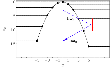
Figure 1: Transition between adjacent spin-energy levels of Hamiltonian (23) mediated by Raman processes.

Then $M_{R}=M_{R}^{(2)}$ and the transition rate is given by

$$\Gamma_{R}^{m\rightarrow m\pm 1}=\sum_{{\scriptsize{\begin{matrix}{\mathbf{k}}\lambda_{\mathbf{k}}\\ {\mathbf{q}}\lambda_{\mathbf{q}}\end{matrix}}}}\frac{2\pi}{\hbar}|M_{R}^{(2)}|^{2}\delta\left(\hbar\omega_{\mathbf{q}}-\hbar\omega_{\mathbf{k}}+E_{m\pm 1}-E_{m}\right)\,.$$ (30)

Note that in the sums over the polarizations $\lambda_{\mathbf{k}}$ and $\lambda_{\mathbf{q}}$, only the two transverse modes are considered. To complete the calculation, we make use of

$$[{\mathbf{k}}\times{\mathbf{e}}_{{\mathbf{k}}t}] = \pm k{\mathbf{e}}_{{\mathbf{k}}t^{\prime}}$$ (31)

$$\sum_{t=t_{1},t_{2}}({\mathbf{e}}_{{\mathbf{k}}t}\cdot{\mathbf{a}})({\mathbf{e}}_{{\mathbf{k}}t}\cdot{\mathbf{b}}) = {\mathbf{a}}\cdot{\mathbf{b}}-\frac{({\mathbf{k}}\cdot{\mathbf{a}})({\mathbf{k}}\cdot{\mathbf{b}})}{k^{2}}\,$$ (32)

and the replacement of $\sum_{\mathbf{k}}$ by $V\int d^{3}k/(2\pi)^{3}$ to obtain

$$\Gamma_{R}^{m\rightarrow m\pm 1}=\frac{1}{\hbar}\frac{l_{m,m\pm 1}^{2}I_{R1}}{\pi^{3}}\frac{[D(-2m\mp 1)]^{2}}{{\cal{E}}^{8}_{t}}(k_{B}T)^{7}\,,$$ (33)

where

$${\cal{E}}_{t}\equiv(\hbar^{3}\rho v_{t}^{5})^{1/4}$$ (34)

is a characteristic energy in the problem. In these expressions $\rho$ is the mass density and $v_{t}$ is velocity of transverse sound. $I_{R1}$ is given by

$$I_{R1}=\frac{1}{1152}\int_{0}^{\theta_{D}/T}dxx^{3}(x+\epsilon_{1})^{3}\frac{e^{x+\epsilon_{1}}}{(e^{x}-1)(e^{x+\epsilon_{1}}-1)}\,,$$ (35)

where

$$\epsilon_{1}=\frac{E_{m}-E_{m\pm 1}}{k_{B}T}=\frac{D(\pm 2m+1)\pm g\mu_{B}H}{k_{B}T}\,.$$ (36)

We remind the reader that in the above formulas the choice of upper and lower sign corresponds the choice of $\pm$ in Eq. (27). We use $m+1$ for positive $m$ and we use $m-1$ for negative $m$, so that $E_{m}-E_{m\pm 1}>0$.

III.1.2 Non-adjacent spin levels, $m\rightarrow m\pm 2$

It is clear from equations (25) and (26) that the only allowed transitions between non-adjacent spin levels are those with

$$|m_{+}\rangle=|m\rangle\,,\qquad|m_{-}\rangle=|m\pm 2\rangle\,.$$ (37)

\begin{picture}(13.0,5.5)\centerline{\hbox{\psfig{width=227.62204pt}}} \end{picture}

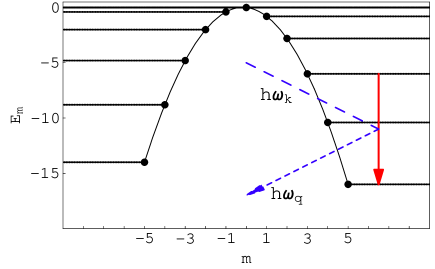
Figure 2: Transition between the spin-energy levels of Hamiltonian (23) $m\rightarrow m+2$ due to Raman scattering.

In this case, represented in Fig. 2, equations (25) and (26) give

$$M_{R}^{(2)}=D\,l_{m,m\pm 1}l_{m\pm 1,m\pm 2}M_{\mathrm{ph-R}}^{\pm\pm}$$

$$M_{R}^{(1+1)}=-\frac{D^{2}}{2}(\pm 2m+3)(\pm 2m+1)\,l_{m,m\pm 1}l_{m\pm 1,m\pm 2}$$

$$\times\left(\frac{M_{\mathrm{ph-R}}^{\pm\pm}}{E_{m\pm 1}-E_{m}+\hbar\omega_{\mathbf{k}}}+\frac{M_{\mathrm{ph-R}}^{\pm\pm}}{E_{m\pm 1}-E_{m}-\hbar\omega_{\mathbf{q}}}\right)\,,$$

where

$$M_{\mathrm{ph-R}}^{--} = \frac{1}{2}\left[M_{\mathrm{ph-R}}^{xx}+i(M_{\mathrm{ph-R}}^{xy}+M_{\mathrm{ph-R}}^{yx})-M_{\mathrm{ph-R}}^{yy}\right]$$

$$M_{\mathrm{ph-R}}^{++} = \frac{1}{2}\left[M_{\mathrm{ph-R}}^{xx}-i(M_{\mathrm{ph-R}}^{xy}+M_{\mathrm{ph-R}}^{yx})-M_{\mathrm{ph-R}}^{yy}\right]\,.$$

The transition rate can be obtained by computing

$$\Gamma_{R}^{m\rightarrow m\pm 2}=\sum_{{\scriptsize{\begin{matrix}{\mathbf{k}}\lambda_{\mathbf{k}}\\ {\mathbf{q}}\lambda_{\mathbf{q}}\end{matrix}}}}\frac{2\pi}{\hbar}|M_{R}|^{2}\delta\left(\hbar\omega_{\mathbf{q}}-\hbar\omega_{\mathbf{k}}+E_{m\pm 2}-E_{m}\right)\,,$$ (40)

with $M_{R}$ given by equations (13) and (III.1.2). Again, we use equations (31) and (32) and the replacement of $\sum_{\mathbf{k}}$ by $Vd^{3}k/(2\pi)^{3}$ (with $V$ being the volume of the crystal) to obtain the final result

$$\Gamma_{R}^{m\rightarrow m\pm 2}=\frac{1}{\hbar}\frac{l_{m,m\pm 1}^{2}l_{m\pm 1,m\pm 2}^{2}\,I_{R2}}{\pi^{3}}\frac{D^{2}}{{{\cal{E}}^{8}_{t}}}(k_{B}T)^{7}\,,$$ (41)

where

$$I_{R2}=\frac{1}{288}\int_{0}^{\theta_{D}/T}dx\frac{(x+\epsilon_{2})^{3}x^{3}e^{(x+\epsilon_{2})}}{[e^{x}-1][e^{(x+\epsilon_{2})}-1]}\bigg{\{}1-$$

$$\frac{1}{2}(\pm 2m+1)(\pm 2m+3)\left[\frac{D/k_{B}T}{\epsilon_{1}+x}+\frac{D/k_{B}T}{\epsilon_{1}-\epsilon_{2}-x}\right]\bigg{\}}^{2}$$

with

$$\epsilon_{2}=\frac{E_{m}-E_{m\pm 2}}{k_{B}T}=\frac{4(\pm m+1)\pm 2g\mu_{B}H}{k_{B}T}\,.$$ (43)

III.2 Transitions between tunnel-split states

Consider now a biaxial spin Hamiltonian with strong uniaxial anisotropy

$${\mathcal{\hat{H}}}_{S}={\mathcal{\hat{H}}}_{A}-g\mu_{B}{\mathbf{H}}\cdot{\mathbf{S}}\,,\qquad{\mathcal{\hat{H}}}_{A}=-DS_{z}^{2}+E[S_{x}^{2}-S_{y}^{2}]\,,$$ (44)

where $D\gg E>0$ and $DS\gg g\mu_{B}H_{\perp}$, with $H_{\perp}$ being the transverse magnetic field. Consequently, ${\mathcal{\hat{H}}}_{A}$ nearly commutes with $S_{z}$. The energy levels of this Hamiltonian are approximately given by Eq. (24). The two levels $m$ and $m^{\prime}$ are in resonance for the values of the magnetic field $H_{z,mm^{\prime}}^{(res)}=(m+m^{\prime})D/(g\mu_{B})$. The level bias is given by

$$W\equiv E_{m}-E_{m}^{\prime}=g\mu_{B}\left(H_{z}-H_{z,mm^{\prime}}^{(res)}\right)(m^{\prime}-m)\,.$$ (45)

\begin{picture}(11.0,5.5)\centerline{\hbox{\psfig{width=227.62204pt}}} \end{picture}

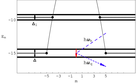
Figure 3: Transition between tunnel-split states due to Raman scattering.

III.2.1 The two state model

Due to the terms in ${\mathcal{\hat{H}}}_{S}$ that do not commute with $S_{z}$, the true eigenstates of ${\mathcal{\hat{H}}}_{S}$ far from a resonance are given by expansions over the complete $|m\rangle$ basis:

$$|\phi_{m}\rangle=\sum_{m^{\prime\prime}=-S}^{S}c_{mm^{\prime\prime}}|m^{\prime\prime}\rangle\,,$$ (46)

where $|c_{mm}|\simeq 1$ and all the other coefficients are small. Hybridization of the states $|\phi_{m}\rangle$ and $|\phi_{m^{\prime}}\rangle$ when they are close to resonance can be taken into account in the framework of the two-state model

$$\left\langle\phi_{m_{i}}\left|{\mathcal{\hat{H}}}_{S}\right|\phi_{m_{i}}\right\rangle=E_{m_{i}},\quad m_{i}=m,m^{\prime}$$

$$\left\langle\phi_{m}\left|{\mathcal{\hat{H}}}_{S}\right|\phi_{m^{\prime}}\right\rangle=\frac{1}{2}\Delta\,,$$ (47)

where $\Delta$ is the tunnel splitting of the levels $m$ and $m^{\prime}$ that can be calculated from the exact spin Hamiltonian ${\mathcal{\hat{H}}}_{S}$ Garanin or determined experimentally. Diagonalizing this $2\times 2$ matrix yields the eigenvalues

$$E_{\pm}=\frac{1}{2}\left(E_{m}+E_{m^{\prime}}\pm\sqrt{W^{2}+\Delta^{2}}\right)\,.$$ (48)

The corresponding eigenvectors can be represented in the form

$$|\psi_{\pm}\rangle=\frac{1}{\sqrt{2}}\left(C_{\pm}|\phi_{m}\rangle\pm C_{\mp}|\phi_{m^{\prime}}\rangle\right)\,,$$ (49)

where

$$C_{\pm}=\sqrt{1\pm\frac{W}{\sqrt{W^{2}+\Delta^{2}}}}\,.$$ (50)

Far from the resonance, $|W|\gg\Delta$, the eigenstates and energy eigenvalues reduce to those of $|\phi_{m}\rangle$ and $|\phi_{m^{\prime}}\rangle$ states.

III.2.2 Matrix elements

Here we consider Raman processes involving spin transitions between tunnel-split states (see Fig. 3). That is, the spin eigenstates in Eq. (11) are given by Eq. (49). In order to compute the matrix element of the Raman process, we can rewrite $M_{R}^{(2)}$ by adding and subtracting ${\mathcal{\hat{H}}}_{Z}$ in the spin matrix element of Eq. (18)

$$\left\langle\psi_{-}\left|\left[\left[{\mathcal{\hat{H}}}_{A},S_{\alpha}\right],S_{\beta}\right]\right|\psi_{+}\right\rangle=\left\langle\psi_{-}\left|\left[\left[{\mathcal{\hat{H}}}_{S},S_{\alpha}\right],S_{\beta}\right]\right|\psi_{+}\right\rangle$$

$$\qquad\qquad\qquad\qquad-\left\langle\psi_{-}\left|\left[\left[{\mathcal{\hat{H}}}_{Z},S_{\alpha}\right],S_{\beta}\right]\right|\psi_{+}\right\rangle\,.$$ (51)

Taking into account that $|\psi_{\pm}\rangle$ are the eigenstates of ${\mathcal{\hat{H}}}_{S}$ and inserting the identity $1=\sum_{\xi}|\psi_{\xi}\rangle\langle\psi_{\xi}|$ we can express the first term of the right hand side as

$$\left\langle\psi_{-}\left|\left[\left[\hat{H}_{S},S_{\alpha}\right],S_{\beta}\right]\right|\psi_{+}\right\rangle=$$

$$\sum_{\xi}\left(E_{-}+E_{+}-2E_{\xi}\right)\left\langle\psi_{-}\left|S_{\alpha}\right|\psi_{\xi}\right\rangle\left\langle\psi_{\xi}\left|S_{\beta}\right|\psi_{+}\right\rangle.\qquad$$ (52)

Then,

$$M_{R}^{(2)}=-\bigg{\{}\sum_{\xi}\left(E_{-}+E_{+}-2E_{\xi}\right)\left\langle\psi_{-}\left|S_{\alpha}\right|\psi_{\xi}\right\rangle\times$$

$$\left\langle\psi_{\xi}\left|S_{\beta}\right|\psi_{+}\right\rangle\,-\left\langle\psi_{-}\left|\left[\left[{\mathcal{\hat{H}}}_{Z},S_{\alpha}\right],S_{\beta}\right]\right|\psi_{+}\right\rangle\bigg{\}}\tilde{M}_{\mathrm{ph-R}}^{\alpha\beta}\,.$$

(53)

Following the same procedure, we can rewrite $M_{R}^{(1+1)}$ from Eq. (22) as an expansion on powers of $H$:

$$M_{R}^{(1+1)}=M_{R}^{(1+1)}(H^{0})+M_{R}^{(1+1)}(H^{1})+O(H^{2})$$ (54)

with

$$M_{R}^{(1+1)}(H^{0})=$$

$$-\sum_{\xi}\left(E_{-}-E_{\xi}\right)\left(E_{\xi}-E_{+}\right)\left\langle\psi_{-}\left|S_{\alpha}\right|\psi_{\xi}\right\rangle\left\langle\psi_{\xi}\left|S_{\beta}\right|\psi_{+}\right\rangle$$

$$\times\left[\frac{M_{\mathrm{ph-R}}^{\alpha\beta}}{E_{+}+\hbar\omega_{\mathbf{k}}-E_{\xi}}+\frac{M_{\mathrm{ph-R}}^{\beta\alpha}}{E_{+}-E_{\xi}-\hbar\omega_{\mathbf{q}}}\right]$$ (55)

and

$$M_{R}^{(1+1)}(H^{1})=$$

$$\sum_{\xi}\frac{\left\langle\psi_{-}\left|\left[\hat{H}_{Z},S_{\alpha}\right]\right|\psi_{\xi}\right\rangle\left\langle\psi_{\xi}\left|\left[\hat{H}_{S},S_{\beta}\right]\right|\psi_{+}\right\rangle}{E_{+}+\hbar\omega_{\mathbf{k}}-E_{\xi}}M_{\mathrm{ph-R}}^{\alpha\beta}$$

$$+\sum_{\xi}\frac{\left\langle\psi_{-}\left|\left[\hat{H}_{S},S_{\alpha}\right]\right|\psi_{\xi}\right\rangle\left\langle\psi_{\xi}\left|\left[\hat{H}_{Z},S_{\beta}\right]\right|\psi_{+}\right\rangle}{E_{+}+\hbar\omega_{\mathbf{k}}-E_{\xi}}M_{\mathrm{ph-R}}^{\alpha\beta}$$

$$+\sum_{\xi}\frac{\left\langle\psi_{-}\left|\left[\hat{H}_{Z},S_{\alpha}\right]\right|\psi_{\xi}\right\rangle\left\langle\psi_{\xi}\left|\left[\hat{H}_{S},S_{\beta}\right]\right|\psi_{+}\right\rangle}{E_{+}-E_{\xi}-\hbar\omega_{\mathbf{q}}}M_{\mathrm{ph-R}}^{\beta\alpha}$$

$$+\sum_{\xi}\frac{\left\langle\psi_{-}\left|\left[\hat{H}_{S},S_{\alpha}\right]\right|\psi_{\xi}\right\rangle\left\langle\psi_{\xi}\left|\left[\hat{H}_{Z},S_{\beta}\right]\right|\psi_{+}\right\rangle}{E_{+}-E_{\xi}-\hbar\omega_{\mathbf{q}}}M_{\mathrm{ph-R}}^{\beta\alpha}.$$

(56)

III.2.3 Transition rate for $H=0$

At $H=0$ one obtains

$$M_{R}=-\sum_{\xi}\left\langle\psi_{-}\left|S_{\alpha}\right|\psi_{\xi}\right\rangle\left\langle\psi_{\xi}\left|S_{\beta}\right|\psi_{+}\right\rangle\left[M_{\mathrm{ph-R}}^{(\alpha\beta)}\times\right.$$

$$\left.\left(\frac{E_{-}+E_{+}}{2}-E_{\xi}+\frac{\left(E_{-}-E_{\xi}\right)\left(E_{\xi}-E_{+}\right)}{E_{+}+\hbar\omega_{\mathbf{k}}-E_{\xi}}\right)+\right.$$

$$\left.M_{\mathrm{ph-R}}^{(\beta\alpha)}\left(\frac{E_{-}+E_{+}}{2}-E_{\xi}+\frac{\left(E_{-}-E_{\xi}\right)\left(E_{\xi}-E_{+}\right)}{E_{+}-E_{\xi}-\hbar\omega_{\mathbf{q}}}\right)\right]$$

(57)

It is convenient to consider the terms with $\xi=\pm$ and $\xi\neq\pm$ separately. The contribution from $\xi=\pm$ is

$$M_{R}=-\left(E_{+}-E_{-}\right)\bigg{(}\left\langle\psi_{-}\left|S_{\alpha}\right|\psi_{-}\right\rangle\left\langle\psi_{-}\left|S_{\beta}\right|\psi_{+}\right\rangle$$

$$-\left\langle\psi_{-}\left|S_{\alpha}\right|\psi_{+}\right\rangle\left\langle\psi_{+}\left|S_{\beta}\right|\psi_{+}\right\rangle\bigg{)}\tilde{M}_{\mathrm{ph-R}}^{\alpha\beta}.$$ (58)

Using the time-reversal symmetry, we obtain

$$\langle\psi_{\pm}|{\mathbf{S}}|\psi_{\pm}\rangle=-\langle\psi_{\pm}|{\mathbf{S}}|\psi_{\pm}\rangle^{*}\,.$$ (59)

For the biaxial model with $E>0$ the states $|\psi_{\pm}\rangle$ are real. Then,

$$\langle\psi_{\pm}|S_{z}|\psi_{\pm}\rangle=\langle\psi_{\pm}|S_{x}|\psi_{\pm}\rangle=0\,.$$ (60)

On the other hand, $\langle\psi_{\pm}|S_{y}|\psi_{\pm}\rangle=0$ because of the factorization of the Hilbert space: $\mathcal{H}=\mathcal{H}_{1}^{(1)}\otimes\mathcal{H}_{1}^{(2)},$ $\left(-S,-S+2,\ldots,S\right)\in\mathcal{H}_{1}^{(1)}$ and $\left(-S+1,-S+3,\ldots,S-1\right)\in\mathcal{H}_{1}^{(2)}$. Thus Eq. (58) yields a zero result.

Let us consider now the terms with $\xi\neq\pm$. In this case, the difference between the energies of the doublet is much smaller than the energy distance to the other states, $|E_{+}-E_{-}|\ll|E_{\pm}-E_{\xi}|$, so that one can replace $E_{\pm}$ with $E$ and $\hbar\omega_{\mathbf{q}}$ with $\hbar\omega_{\mathbf{k}}$ in the matrix elements. We consider the case of low temperature, when $\hbar\omega_{\mathbf{k}}\ll\left|E-E_{\xi}\right|$ for thermal phonons. Then $M_{R}$ can be simplified to

$$M_{R}\simeq 2\left(\hbar\omega_{\mathbf{k}}\right)^{2}\tilde{M}_{\mathrm{ph-R}}^{\alpha\beta}A_{\alpha\beta}\,,$$ (61)

with

$$A_{\alpha\beta}\equiv\sum_{\xi}{}^{{}^{\prime}}\frac{\left\langle\psi_{-}\left|S_{\alpha}\right|\psi_{\xi}\right\rangle\left\langle\psi_{\xi}\left|S_{\beta}\right|\psi_{+}\right\rangle}{E-E_{\xi}},$$ (62)

where prime means that $\xi=\pm$ have been excluded. Note that the quadratic dependence on $\omega_{\mathbf{q}}$ in Eq. (61) results from cancellations between terms from $M_{R}^{(2)}$ and terms from $M_{R}^{(1+1)}$. Consequently, the relaxation rate will have a different temperature dependence from the result that one would obtain if one added the rates stemming from $M_{R}^{(2)}$ and $M_{R}^{(1+1)}$ independently. The rate is given by

$$\Gamma_{R0}^{+\rightarrow-}=\sum_{{\mathbf{k}},\lambda_{\mathbf{k}}}\sum_{{\mathbf{q}},\lambda_{\mathbf{q}}}\frac{2\pi}{\hbar}|M_{R}|^{2}\delta\left(\hbar\omega_{\mathbf{q}}-\hbar\omega_{\mathbf{k}}\right)$$

$$=\frac{1}{18\hbar\left(2\pi\right)^{3}}\sum_{\alpha\beta}A_{\alpha\beta}\left(A_{\alpha\beta}^{*}+A_{\beta\alpha}^{*}\right)\frac{(k_{B}T)^{11}}{{{\cal{E}}^{8}_{t}}}I_{10}$$

(63)

where equations (31) and (32) have been used and the continuum limit has been taken. The constant $I_{10}$ is

$$I_{10}=\int_{0}^{\infty}dx\,\frac{x^{10}e^{x}}{\left(e^{x}-1\right)^{2}}=\Gamma(11)\zeta(10).$$ (64)

For transitions between the lowest doublet $m=-S,m^{\prime}=S$ specified in Eq. (49) one can evaluate $A_{\alpha\beta}$ by considering also the first excited doublet $m=-S+1,m^{\prime}=S-1$

$$\left|\psi_{1\pm}\right\rangle=\frac{1}{\sqrt{2}}\left(C_{1\pm}\left|\phi_{m+1}\right\rangle\pm C_{1\mp}\left|\phi_{{m}^{\prime}-1}\right\rangle\right)$$ (65)

with $C_{1\pm}$ given by Eq. (50) with $\Delta\rightarrow\Delta_{1}$ and $W\rightarrow W_{1}$. Hence the only non zero matrix elements are

$$A_{\pm\mp}=\frac{1}{E_{m}-E_{m+1}}\bar{A}_{\pm\mp},$$ (66)

where

$$\bar{A}_{\pm\mp}\equiv\sum_{\eta=\pm}\left\langle\psi_{-}\left|S_{\pm}\right|\psi_{1\eta}\right\rangle\left\langle\psi_{1\eta}\left|S_{\mp}\right|\psi_{+}\right\rangle.$$ (67)

Evaluation of these matrix elements yields

$$\sum_{\alpha\beta}A_{\alpha\beta}\left(A_{\alpha\beta}^{*}+A_{\beta\alpha}^{*}\right)=\frac{S^{2}}{\left(E_{-S}-E_{-S+1}\right)^{2}}\frac{\Delta^{2}}{W^{2}+\Delta^{2}}\,.$$ (68)

For the case under consideration $W=0$ and the transition rate is, then

$$\Gamma_{R0}^{+\rightarrow-}=\frac{80\,\pi^{7}S^{2}}{297\hbar}\frac{(k_{B}T)^{11}}{\left(E_{-S}-E_{-S+1}\right)^{2}{{\cal{E}}^{8}_{t}}}.$$ (69)

III.2.4 Transition rate in the presence of a magnetic field

Here we are going to evaluate the contribution of the magnetic field ${\mathbf{H}}$ to the rate of the transition between the tunnel-split ground-state levels. We consider magnetic fields with very small longitudinal component, $g\mu_{B}H_{z}\sim\Delta$. For longitudinal fields $g\mu_{B}H_{z}\gg\Delta$ the Raman processes die out. We are also restricted to not very large transverse magnetic fields, $g\mu_{B}H_{\perp}\ll DS$. In this case, it is sufficient to compute the lowest-order contribution of the magnetic field to the transition rate. This contribution can be essential because of the cancellation that occurs in the matrix element for the $H=0$ case, Eq. (61). This cancellation leads to the $\Gamma_{R}^{+\rightarrow-}\propto T^{11}$ dependence. As we shall see, there is no such cancellation in the field-dependent term, so that the result shows a $T^{7}$-dependence.

According to Eq. (53), the linear order contribution of $H$ to $M_{R}^{(2)}$ is given by

$$\delta M_{R}^{(2)}=\left\langle\psi_{-}\left|\left[\left[\hat{H}_{Z},S_{\alpha}\right],S_{\beta}\right]\right|\psi_{+}\right\rangle\tilde{M}_{\mathrm{ph-R}}^{\alpha\beta}\,.$$ (70)

The double commutator equals

$$\left[\left[\hat{H}_{Z},S_{\alpha}\right],S_{\beta}\right]=g\mu_{B}\left(H_{\beta}S_{\alpha}-H_{\gamma}S_{\gamma}\delta_{\alpha\beta}\right)$$ (71)

so that

$$\delta M_{R}^{(2)} = g\mu_{B}\left(H_{\beta}\delta_{\alpha z}-H_{z}\delta_{\alpha\beta}\right)\tilde{M}_{\mathrm{ph-R}}^{\alpha\beta}\left\langle\psi_{-}\left|S_{z}\right|\psi_{+}\right\rangle$$ (72)

$$= g\mu_{B}K_{\alpha\beta}^{(2)}\tilde{M}_{\mathrm{ph-R}}^{\alpha\beta},$$

where

$$K_{\alpha\beta}^{(2)}=-\left(H_{\beta}\delta_{\alpha z}-H_{z}\delta_{\alpha\beta}\right)\frac{\Delta}{\sqrt{W^{2}+\Delta^{2}}}\frac{m^{\prime}-m}{2}.$$ (73)

The phonon matrix element $\tilde{M}_{\mathrm{ph-R}}^{\alpha\beta}$ is symmetric in $\alpha\beta$. Thus, it is possible and convenient to replace $K_{\alpha\beta}^{(2)}$ in Eq. (72) by the symmetrized tensor

$$\tilde{K}_{\alpha\beta}^{(2)}=\frac{1}{2}\left(K_{\alpha\beta}^{(2)}+K_{\beta\alpha}^{(2)}\right)\,.$$ (74)

On the other hand, the linear order contribution of $H$ to $M_{R}^{(1+1)}$ is given by Eq. (56). By using Eq. (71) and assuming $\hbar\omega_{\mathbf{k}}\ll E_{m+1}-E_{m}$ we obtain

$$\delta M_{R}^{(1+1)} \cong ig\mu_{B}2H_{\gamma}\left(\epsilon_{\gamma\alpha\delta}\bar{A}_{\delta\beta}-\epsilon_{\gamma\beta\delta}\bar{A}_{\alpha\delta}\right)\tilde{M}_{\mathrm{ph-R}}^{\alpha\beta}$$ (75)

$$\equiv g\mu_{B}K_{\alpha\beta}^{(1+1)}\tilde{M}_{\mathrm{ph-R}}^{\alpha\beta},$$

where

$$K_{\alpha\beta}^{(1+1)}=i2H_{\gamma}\left(\epsilon_{\gamma\alpha\delta}\bar{A}_{\delta\beta}-\epsilon_{\gamma\beta\delta}\bar{A}_{\alpha\delta}\right).$$ (76)

Again, it is convenient to replace $K_{\alpha\beta}^{(1+1)}$ in Eq. (75) by the symmetrized version

$$\tilde{K}_{\alpha\beta}^{(1+1)}=\frac{1}{2}\left(K_{\alpha\beta}^{(1+1)}+K_{\beta\alpha}^{(1+1)}\right)\,.$$ (77)

The addition to the Raman matrix element due to $H\neq 0$ is, then

$$\delta M_{R}\equiv\delta M_{R}^{(2)}+\delta M_{R}^{(1+1)}=g\mu_{B}\tilde{K}_{\alpha\beta}\tilde{M}_{\mathrm{ph-R}}^{\alpha\beta}\,,$$ (78)

with $\tilde{K}_{\alpha\beta}=\tilde{K}_{\alpha\beta}^{(2)}+\tilde{K}_{\alpha\beta}^{(1+1)}$. The transition rate is based upon $|M_{R}+\delta M_{R}|^{2}$. Here, $|M_{R}|^{2}$ was taken into account above. The interference term can be shown to be proportional to $H_{z}$ and thus negligibly small. Therefore, the field effect is entirely contained in the term $|\delta M_{R}|^{2}$. Applying the same procedure as in the previous section, one obtains the following addition to the relaxation rate

$$\delta\Gamma_{R}^{+\rightarrow-}=\frac{1}{\hbar}\frac{\pi^{3}}{3024}\left(g\mu_{B}\right)^{2}\sum_{\alpha\beta}|\tilde{K}_{\alpha\beta}|^{2}\frac{(k_{B}T)^{7}}{{{\cal{E}}^{8}_{t}}}.$$ (79)

Evaluation of $\sum_{\alpha\beta}|\tilde{K}_{\alpha\beta}|^{2}$ for the lowest doublet $m=-S,m^{\prime}=S$ yields

$$\sum_{\alpha\beta}|\tilde{K}_{\alpha\beta}|^{2}=2\left(H_{z}^{2}+\frac{1}{4}H_{\perp}^{2}\right)\frac{\Delta^{2}}{W^{2}+\Delta^{2}}\,S^{2}\,.$$ (80)

Therefore, the transition rate in the presence of a magnetic field is

$$\Gamma_{R}^{+\rightarrow-}({\mathbf{H}})\simeq\frac{\Delta^{2}}{W^{2}+\Delta^{2}}\,\left(\Gamma_{R0}^{+\rightarrow-}+\delta\Gamma_{R0}^{+\rightarrow-}\right)\,,$$ (81)

where $\Gamma_{R0}^{+\rightarrow-}$ is given by Eq. (69) and

$$\delta\Gamma_{R0}^{+\rightarrow-}=\frac{\pi^{3}S^{2}}{6048\hbar}\frac{H_{\perp}^{2}\left(g\mu_{B}\right)^{2}(k_{B}T)^{7}}{{{\cal{E}}^{8}_{t}}}\,.$$ (82)

Note that we have used $H_{z}\ll H_{\perp}$ in the last expression. One can see from Eq. (81) that the relaxation rate due to Raman processes dies out when going out of resonance, $W\gg\Delta$.

IV Processes involving emission of two phonons

For processes involving emission of two phonons of, say, wave vectors $\mathbf{k}$ and $\mathbf{q}$ we use the following designations:

$$\left|\phi_{+}\right\rangle\equiv\left|n_{\mathbf{k}},n_{\mathbf{q}}\right\rangle,\qquad\left|\phi_{-}\right\rangle\equiv\left|n_{\mathbf{k}}+1,n_{\mathbf{q}}+1\right\rangle$$ (83)

In this case, conservation of energy reads:

$$E_{+}-E_{-}=\hbar\omega_{\mathbf{k}}+\hbar\omega_{\mathbf{q}}.$$ (84)

The matrix element for this process is, again, the sum of the matrix element with $\hat{{\mathcal{H}}}_{\mathrm{s-ph}}^{(2)}$ and that with $\hat{{\mathcal{H}}}_{\mathrm{s-ph}}^{(1)}$ in the second order:

$$M_{E}=M_{E}^{(2)}+M_{E}^{(1+1)},$$ (85)

where according to equations (II) and (14),

$$M_{E}^{(2)}=-\frac{1}{2}\left\langle\psi_{-}\left|\left[\left[\hat{{\mathcal{H}}}_{A},S_{\alpha}\right],S_{\beta}\right]\right|\psi_{+}\right\rangle$$

$$\qquad\times\left\langle n_{\mathbf{k}}-1,n_{\mathbf{q}}+1\left|\delta\phi_{\alpha}\delta\phi_{\beta}\right|n_{\mathbf{k}},n_{\mathbf{q}}\right\rangle.$$ (86)

In this case it is convenient to express the phonon matrix element as:

$$\left\langle n_{\mathbf{k}}+1,n_{\mathbf{q}}+1\left|\delta\phi_{\alpha}\delta\phi_{\beta}\right|n_{\mathbf{k}},n_{\mathbf{q}}\right\rangle$$

$$=M_{\mathrm{ph-E}}^{\alpha\beta}+M_{\mathrm{ph-E}}^{\beta\alpha}\equiv 2\tilde{M}_{\mathrm{ph-E}}^{\alpha\beta},$$ (87)

where

$$M_{\mathrm{ph-E}}^{\alpha\beta}=\left\langle n_{\mathbf{q}}+1\left|\delta\phi_{\alpha}\right|n_{\mathbf{q}}\right\rangle\left\langle n_{\mathbf{k}}+1\left|\delta\phi_{\beta}\right|n_{\mathbf{k}}\right\rangle$$

$$=\frac{\hbar^{2}}{8\rho V}\frac{\left[\mathbf{k}\times\mathbf{e}_{\mathbf{k}\lambda_{\mathbf{k}}}\right]_{\alpha}\left[\mathbf{q}\times\mathbf{e}_{\mathbf{q}\lambda_{\mathbf{q}}}\right]_{\beta}}{\sqrt{\hbar\omega_{\mathbf{k}\lambda_{\mathbf{k}}}\hbar\omega_{\mathbf{q}\lambda_{\mathbf{q}}}}}\sqrt{\left(n_{\mathbf{q}}+1\right)(n_{\mathbf{k}}+1)}.$$

IV.1 Transitions between eigenstates of $S_{z}$

As stated above, the spin-phonon relaxation by emission of two phonons may be more important than the relaxation by Raman processes only if the energy difference between the spin-states satisfies $\Delta E\ll k_{B}T$. Provided that the energy difference between tunnel-split levels, $\Delta$, is very small, only the relaxation by the emission of two phonons between eigenstates of $Sz$ will be considered.

To this end, we will make use of the spin-Hamiltonian (23) and the transitions between its eigenstates, $|m\rangle$.

IV.1.1 Adjacent spin levels, $m\rightarrow m\pm 1$

The matrix elements in this case are

$$M_{E}^{(2)}=D(\mp 2m+1)l_{m,m\pm 1}\tilde{M}_{\mathrm{ph-E}}^{z\pm}$$

$$M_{E}^{(1+1)}=0\,,$$ (89)

with

$$\tilde{M}_{\mathrm{ph-E}}^{z\pm}=\frac{1}{2}\left[\tilde{M}_{\mathrm{ph-E}}^{zx}\mp i\tilde{M}_{\mathrm{ph-E}}^{zy}\right]\,.$$ (90)

The decay rate is then given by

$$\Gamma_{E}^{m\rightarrow m\pm 1}=\sum_{{\scriptsize{\begin{matrix}{\mathbf{k}}\lambda_{\mathbf{k}}\\ {\mathbf{q}}\lambda_{\mathbf{q}}\end{matrix}}}}\frac{2\pi}{\hbar}|M_{E}^{(2)}|^{2}\delta\left(\hbar\omega_{\mathbf{k}}+\hbar\omega_{\mathbf{q}}+E_{m\pm 1}-E_{m})\right).$$ (91)

Using the same techniques as in the previous calculations, one obtains

$$\Gamma_{E}^{m\rightarrow m\pm 1}=\frac{1}{\hbar}\frac{l_{m,m\pm 1}^{2}I_{E1}}{\pi^{3}}\frac{\left[D(2m\pm 1)\right]^{2}}{{{\cal{E}}^{8}_{t}}}(k_{B}T)^{7}\,,$$ (92)

where

$$I_{E1}=\frac{1}{1152}\int_{0}^{\epsilon_{1}}dx\frac{x^{3}(\epsilon_{1}-x)^{3}e^{\epsilon_{1}}}{(e^{x}-1)(e^{(\epsilon_{1}-x)}-1)}\,.$$ (93)

IV.1.2 Non-adjacent spin levels, $m\rightarrow m\pm 2$

In this case, the matrix elements are

$$M_{E}^{(2)}=D\,l_{m,m\pm 1}l_{m\pm 1,m\pm 2}{M}_{\mathrm{ph-E}}^{\pm\pm}$$

$$M_{E}^{(1+1)}=-\frac{D^{2}}{2}(\pm 2m+3)(\pm 2m+1)\,l_{m,m\pm 1}l_{m\pm 1,m\pm 2}$$

$$\times\left(\frac{M_{\mathrm{ph-E}}^{\pm\pm}}{E_{m\pm 1}-E_{m}+\hbar\omega_{\mathbf{k}}}+\frac{M_{\mathrm{ph-E}}^{\pm\pm}}{E_{m\pm 1}-E_{m}-\hbar\omega_{\mathbf{q}}}\right)\,,$$

where

$${M}_{\mathrm{ph-E}}^{\pm\pm}=\frac{1}{2}\left[{M}_{\mathrm{ph-E}}^{xx}-{M}_{\mathrm{ph-E}}^{yy}\mp i({M}_{\mathrm{ph-E}}^{xy}+{M}_{\mathrm{ph-E}}^{yx})\right]\,.$$ (95)

The decay rate is

$$\Gamma_{E}^{m\rightarrow m\pm 2}=\frac{1}{\hbar}\frac{l_{m,m\pm 1}^{2}l_{m\pm 1,m\pm 2}^{2}I_{E2}}{\pi^{3}}\frac{D^{2}(k_{B}T)^{7}}{{{\cal{E}}^{8}_{t}}}\,,$$ (96)

with

$$I_{E2}=\frac{1}{288}\int_{0}^{\epsilon_{2}}dx\frac{(\epsilon_{2}-x)^{3}x^{3}e^{\epsilon_{2}}}{[e^{x}-1][e^{(\epsilon_{2}-x)}-1]}\bigg{\{}1-$$

$$\frac{1}{2}(\pm 2m+1)(\pm 2m+3)\left[\frac{D/k_{B}T}{\epsilon_{1}+x}+\frac{D/k_{B}T}{\epsilon_{1}+\epsilon_{2}-x}\right]\bigg{\}}^{2}\,.$$

V Discussion

Let us now compare transition rates obtained for direct, or one-phonon, processes CGS ; Book and the rates of the same transitions due to Raman processes.

For spin transitions between adjacent eigenstates of the spin Hamiltonian (23), the ratio of the Raman rate and the direct rate is given by

$$\frac{\Gamma_{R}^{m\rightarrow m+1}}{\Gamma_{D}^{m\rightarrow m+1}}=\frac{24I_{R1}}{\pi^{2}}\frac{(k_{B}T)^{7}[1-e^{-{\Delta E}/({k_{B}T})}]}{{\cal{E}}_{t}^{4}(\Delta E)^{3}}\,,$$ (98)

where $\Delta E\equiv E_{m}-E_{m+1}$. In the limit of $k_{B}T\ll\Delta E<\theta_{D}$ transitions are dominated by direct processes. When $\Delta E\ll k_{B}T<\theta_{D}$ one has

$$\frac{\Gamma_{R}^{m\rightarrow m+1}}{\Gamma_{D}^{m\rightarrow m+1}}\sim\left(\frac{{\cal{E}}_{t}}{\Delta E}\right)^{2}\left(\frac{k_{B}T}{{\cal{E}}_{t}}\right)^{6}\,.$$ (99)

In this case transitions can be easily dominated by the Raman processes. For example, for $S=10$, $m=5$, $D=0.1$K, $g\mu_{B}H=1K$ the energy difference is $\Delta E=2.1$K, so that at $T=35K$ the rate of the direct process is $\Gamma_{D}^{m\rightarrow m+1}\simeq 10^{5}s^{-1}$, while the rate of the Raman process is $\Gamma_{R}^{m\rightarrow m+1}\simeq 10^{6}s^{-1}$. In these estimates we used the value of ${\cal{E}}_{t}\sim 100$K. Note that in such molecular magnets as Mn-12 and Fe-8 it will be difficult to have the corresponding Raman processes dominant because of large distances between adjacent spin levels and small Debye temperature. Processes involving the emission of two phonons cannot be dominant in any temperature range. In some range they can dominate over Raman processes but not over direct processes.

For spin transitions between tunnel-split states of the spin Hamiltonian (44) at $H=0$, the ratio of the Raman rate over the direct rate at $\Delta\ll k_{B}T$ is given by

$$\frac{\Gamma_{R0}^{+\rightarrow-}}{\Gamma_{D}^{+\rightarrow-}}=\frac{960\pi^{8}}{297(2S-1)^{2}}\;\left(\frac{k_{B}T}{D}\right)^{2}\left(\frac{k_{B}T}{{\cal{E}}_{t}}\right)^{4}\left(\frac{k_{B}T}{\Delta}\right)^{4}\,.$$ (100)

Consequently, in zero field and temperatures significantly exceeding $\Delta$, the Raman processes will have much higher probability than direct processes. At, e.g., $D=0.5$K, $S=10$, $\Delta=10^{-2}$K and $T=5$K, the rate of the direct process gives $\Gamma_{D}^{+\rightarrow-}\simeq 10^{-4}s^{-1}$, while the rate of the Raman process will be $\Gamma_{R}^{+\rightarrow-}\simeq 5\cdot 10^{4}s^{-1}$. Note that at temperatures where Raman processes dominate over direct processes, contribution of the magnetic field to the rate, Eq. (82), is small compared to the zero-field rate, Eq. (69).

CC thanks Jaroslav Albert for useful discussions. This work has been supported by the NSF Grant No. EIA-0310517.

References

• (1) I. Waller, Z. Phys. 79, 370 (1932).
• (2) W. Heitler and E. Teller, Proc. R. Soc. A 281, 340 (1936).
• (3) R. de L. Kronig, Physica 6, 33 (1939).
• (4) J. H. Van Vleck, Phys. Rev. 57, 426 (1940).
• (5) R. Orbach, Proc. R. Soc. A 264, 458 (1961)
• (6) A. Abragam and B. Bleaney, Electron paramagnetic resonance of transition ions, Clarendon Press (1970).
• (7) E. M. Chudnovsky, Phys. Rev. Lett. 72, 3433 (1994).
• (8) E. M. Chudnovsky, D. A. Garanin, and R. Schilling, Phys. Rev. B 72, 94426 (2005) and references therein.
• (9) E. M. Chudnovsky and J. Tejada Palacios, Magnetism in Solids, Rinton Press (2006).
• (10) E. M. Chudnovsky and X. Martinez Hidalgo, Phys. Rev. B 66, 054412 (2002).
• (11) D.A. Garanin, J. Phys. A 24, L61 (1991).
• (12) J. J. Sakurai, Modern Quantum Mechanics, Adison-Wesley Publishing Company (1994).