Phonon-induced relaxation of a two-state system in solids

Abstract

We study phonon-induced relaxation of quantum states of a particle (e.g., electron or proton) in a rigid double-well potential in a solid. Relaxation rate due to Raman two-phonon processes have been computed. We show that in a two-state limit, symmetry arguments allow one to express these rates in terms of independently measurable parameters. In general, the two-phonon processes dominate relaxation at higher temperature. Due to parity effect in a biased two-state system, their rate can be controlled by the bias.

I Introduction

Relaxation and decoherence in a two state system coupled to environment is a fundamental problem of quantum physics. It was intensively studied in the past; see, e.g., the review of Leggett et al. Leggett-review . In the last years the interest to this problem has been revived by the effort to build solid state qubits. Recently, symmetry implications have been considered for the problem of a particle in a rigid double-well potential embedded in a solid Chudnovsky . It was demonstrated that symmetry arguments allow one to obtain parameter-free lower bound on the relaxation of quantum oscillations in a rigid double well, caused by the elastic environment. One of the arguments is that the double-well potential formed by the local arrangement of atoms in a solid is defined in the coordinate frame of that local atomic environment, not in the laboratory frame. Another argument is that interactions of the tunneling variable with phonons must be invariant with respect to global translations and rotations. When these arguments were taken into account, a simple universal result for the relaxation rate was obtained Chudnovsky in terms of measurable constants of the solid, with no unknown interaction constants.

The above mentioned universal result refers to the low temperature limit when the relaxation of a two state system is dominated by the decay of the excited state due to the emission of one phonon. In this paper we extend the method developed in Ref. Chudnovsky, to the study of two-phonon Raman processes in double-well structures Fujisawa1 ; Fujisawa2 ; Wiel ; Ortner ; Naber ; Graber . Such processes can dominate relaxation at higher temperatures Orbach ; Stoof ; Brandes . We will show that in the temperature range bounded by the level splitting from below and by the Debye temperature from above, the rate of the Raman process for a biased rigid double well is given by a universal expression, very much like the rate of the direct one-phonon process. The Raman rate is proportional to the seventh power of temperature, while the one-phonon rate is linear on temperature. Interestingly, however, at small bias, the Raman rate, unlike the one-phonon rate, is proportional to the square of the bias. Consequently Raman processes can be switched on and off by controlling the bias. This universal result, which is a consequence of the parity of quantum states, must have important implications for solid-state qubits at elevated temperatures. Indeed, for an electron in a quantum dot, the rate of a direct one-phonon process is usually small. If the rate of a two-phonon process can be made small as well, this means that one can eliminate phonons as a significant source of relaxation and decoherence of the electron states in solid-state qubits.

II Particle and phonons

Throughout this paper we shall use units where $\hbar=k_{B}=1$ unless stated otherwise. In the absence of phonons, the Hamiltonian in the laboratory frame is

$${\mathcal{H}}_{o}=\frac{\mathbf{p}^{2}}{2m}+{V(\mathbf{r)}}\,,$$ (1)

where $\mathbf{r}$ is the radius vector, $\mathbf{p}$ is the momentum, and ${m}$ is the mass of the particle (e.g., electron). A long-wave phonon described by the displacement field $\mathbf{u(r)}$ translates the rigid double well in space. The Hamiltonian of the system (including the free phonon field) in the laboratory frame becomes

$${\mathcal{H}}={\frac{\mathbf{p}^{2}}{2m}}+{V(\mathbf{r-u)}}+{\mathcal{H}}_{ph}\ .\$$ (2)

Here, ${{\mathcal{H}}_{ph}\ }$ is the Hamiltonian of the free phonon field. We intend to obtain a Hamiltonian of the form ${{\mathcal{H}}={{\mathcal{H}}_{o}}+{{\mathcal{H}}_{ph}}+{\mathcal{H}}_{e-ph}}$ where the last term describes the interaction of phonons with the electron in the double well potential. Using the fact that $\mathbf{u}$ is small, one can expand ${V(\mathbf{r-u)}}$ in Taylor series to obtain

$${\mathcal{H}}={\frac{\mathbf{p}^{2}}{2m}}+{V(\mathbf{r)}}+{\mathcal{H}}_{ph}-{\frac{\partial{V}}{\partial{r_{i}}}}{u_{i}}+{\frac{1}{2!}}{\frac{\partial^{2}{V}}{\partial{r_{i}}\partial{r_{j}}}}{u_{i}}{u_{j}}\ +\ldots\$$ (3)

The first three terms form the interaction-free part of the total Hamiltonian. The rest of the terms containing powers of $\mathbf{u}$ comprise the electron phonon interaction. It is clear that Eq. (3) requires detailed knowledge of the potential and its derivatives. One can, however, obtain Eq. (2) by performing a unitary transformation on Eq. (1) with the help of translation operator $\mathcal{R}{=e^{{i}\mathbf{p}\cdot\mathbf{u}}}$

$${\mathcal{H}}={e^{{-i}\mathbf{p}\cdot\mathbf{u}}}\ \mathcal{H}_{o}{e^{{i}\mathbf{p}\cdot\mathbf{u}}}+{{\mathcal{H}}_{ph}}\,.\$$ (4)

This can be expanded for small $\mathbf{u}$ as

$${\mathcal{H}} = {\mathcal{H}}_{o}+{\mathcal{H}}_{ph}\ +$$ (5)

$$+ {i[{\mathcal{H}}_{o}\,,{p_{i}}]u_{i}}+{\frac{i^{2}}{2}[[{\mathcal{H}}_{o}\,,{p_{i}}],p_{j}]u_{i}u_{j}}+\ldots\ .$$

Working out the commutators brings one back to Eq. (3). However, the use of Eq. (5) that we are going to employ allows one to obtain parameter-free results solely in terms of the energy levels of our effective two-state system without knowledge of the explicit form of $V(\mathbf{r})$.

We consider the case in which the particle, with good accuracy, is localized near $\mathbf{r}=\pm\mathbf{R}_{o}$, where $\pm\mathbf{R}_{o}$ are the energy minima of the left or right wells. Without loss of generality we assume that $\pm\mathbf{R}_{o}=\pm X_{o}\mathbf{e}_{x}$. The localization length of the state inside each well is small compared to the distance between the minima of the double-well potential. The bare ground states (when tunneling is neglected) in the left and right wells, that we denote by $|\pm X_{o}\rangle$, are approximately orthonormal,

$$\langle\pm X_{o}|\pm X_{o}\rangle=1\,,\quad\langle-X_{o}|X_{o}\rangle=0\,.$$ (6)

The tunneling between the wells leads to the hybridization of the states given by orthonormal wave functions

$$\left|\psi_{\pm}\right\rangle=\frac{1}{\sqrt{2}}(C_{\pm}\left|{X}_{o}\right\rangle\mp C_{\mp}\left|{-X}_{o}\right\rangle)$$ (7)

where

$$C_{\pm}=\sqrt{1\pm\varepsilon/\Delta}\,,\qquad\Delta=\sqrt{\Delta_{o}^{2}+\varepsilon^{2}}$$ (8)

with $\Delta_{o}$ being the tunnel splitting in the unbiased double well and $\varepsilon$ being the energy bias between the wells. Note that the double well also has states, $|\psi_{\xi}\rangle$, with energies, $E_{\xi}$, other then $E_{\pm}$ corresponding to $\left|\psi_{\pm}\right\rangle$. The energy splitting

$$\Delta=E_{+}-E_{-}$$ (9)

is considered small compared to the distance from $E_{\pm}$ to other $E_{\xi}$. As we shall see, in this limit the summation over all states $|\psi_{\xi}\rangle$ renders result for phonon-induced transitions between $\left|\psi_{\pm}\right\rangle$ that is insensitive to the explicit form of the potential.

Below we shall deal with the matrix elements of operators $p\equiv p_{x}$, $x$, and their combinations. Other components of $\mathbf{p}$ and $\mathbf{r}$ are irrelevant. Localization of $\left|\psi_{\pm}\right\rangle$ allows one to compute matrix elements of powers of the operator $x$ with the help of the relation

$$x|\pm X_{o}\rangle=\pm X_{o}|\pm X_{o}\rangle\,.$$ (10)

This gives

$$\langle\psi_{\pm}|x|\psi_{\pm}\rangle=X_{o}\frac{1}{2}(C_{+}^{2}-C_{-}^{2})=X_{o}({\varepsilon}/{\Delta})$$

$$\langle\psi_{-}|x|\psi_{+}\rangle=X_{o}C_{+}C_{-}=X_{o}({\Delta}_{o}/{\Delta})$$

$$\langle\psi_{\pm}|x^{2}|\psi_{\pm}\rangle=X_{o}^{2}\,,\quad\langle\psi_{-}|x^{2}|\psi_{+}\rangle=0\,.$$ (11)

To compute other matrix elements we shall use relations

$$p=m\dot{x}=-im[x,{{\mathcal{H}}_{o}}]$$ (12)

and

$$px+xp=m(\dot{x}x+x\dot{x})=m\frac{dx^{2}}{dt}=-im[x^{2},{{\mathcal{H}}_{o}}]\,.$$ (13)

This gives

$$\langle\psi_{\xi}|p|\psi_{\xi^{\prime}}\rangle=im(E_{\xi}-E_{\xi^{\prime}})\langle\psi_{\xi}|x|\psi_{\xi^{\prime}}\rangle$$

$$\langle\psi_{\xi}|p\,x+xp|\psi_{\xi^{\prime}}\rangle=im(E_{\xi}-E_{\xi^{\prime}})\langle\psi_{\xi}|x^{2}|\psi_{\xi^{\prime}}\rangle$$ (14)

and thus, $\langle\psi_{-}|px|\psi_{+}\rangle=0$.

As we shall see, perturbation theory for Raman processes requires computation of the sum

$$\Sigma={\sum_{\xi\neq+}}\frac{\langle\psi_{-}|p|\psi_{\xi}\rangle\langle\psi_{\xi}|p|\psi_{+}\rangle}{E_{\xi}-E_{+}}\,.$$ (15)

Application of Eq. (12) eliminates the denominator and yields

$$\Sigma=im{\sum_{\xi\neq+}}\langle\psi_{-}|p|\psi_{\xi}\rangle\langle\psi_{\xi}|x|\psi_{+}\rangle\,.$$ (16)

Using the completeness of $|\psi_{\xi}\rangle$ we obtain

$$\Sigma=im[\langle\psi_{-}|px|\psi_{+}\rangle-\langle\psi_{-}|p|\psi_{+}\rangle\langle\psi_{+}|x|\psi_{+}\rangle]\,.$$ (17)

Finally, with the help of the above relations for matrix elements of $x$, $p$, and $px$ we get

$$\Sigma=-m^{2}X_{o}^{2}(\Delta_{o}/\Delta)\varepsilon\,.$$ (18)

This is a mechanism of elimination of unspecified energy levels $E_{\xi}$ from the problem, leading to a universal result.

III Raman matrix element

We are interested in the transition rate between the eigenstates of ${{\mathcal{H}}_{o}+{\mathcal{H}}_{ph}\ }$

$$\left|\Psi_{\pm}\right\rangle=\left|\psi_{\pm}\right\rangle\otimes\left|\phi_{\pm}\right\rangle.\$$ (19)

Here, ${\left|\psi_{\pm}\right\rangle}$ are the tunnel split states of the double well given by Eq. (7). The states ${\left|\phi_{\pm}\right\rangle}$ are the eigenstates of ${{\mathcal{H}}_{ph}\ }$ with energies ${{E_{ph,\pm}}}$. Our goal is to study Raman scattering processes involving absorption of a phonon of frequency ${\omega_{\mathbf{k}}}$ and emission of a phonon of frequency ${\omega_{\mathbf{q}}}={\omega_{\mathbf{k}}+\Delta}$, accompanied by the transition of the particle $\left|\psi_{+}\right\rangle\rightarrow\left|\psi_{-}\right\rangle,$ see Fig.1.

\begin{picture}(18.0,3.5)\centerline{\hbox{\psfig{width=219.08612pt}}} \end{picture}

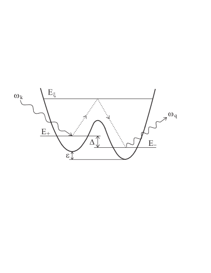
Figure 1: Raman process on tunnel-split levels in a double-well potential, including virtual transitions to higher levels $E_{\xi}$ [the first term in Eq. (24) shown].

The Raman rate can be computed with the help of the Fermi golden rule in the second order in the interaction. The matrix element for this process is the sum of two matrix elements,

$${M=M^{(2)}+M^{(1+1)}}.$$ (20)

The first term denotes the first order perturbation on

$$\mathcal{H}_{e-ph}^{(2)}=-\frac{1}{2}\ {[}[\mathcal{H}{{}_{o}},{p}],{p}{]u_{x}^{2}},\$$ (21)

while the second term stands for the second order perturbation on

$$\mathcal{H}_{e-ph}^{(1)}={i}[\mathcal{H}{{}_{o}},{p}]{u_{x}}.$$ (22)

The explicit expressions for ${M^{(2)}}$ and ${M^{(1+1)}}$ are BHl

$$M^{(2)}=\left\langle\Psi_{-}\right|\mathcal{H}_{e-ph}^{(2)}\left|\Psi_{+}\right\rangle\$$ (23)

and

$$M^{(1+1)} = \sum_{\xi}\ {\frac{\left\langle\Psi_{-}\right|\mathcal{H}_{e-ph}^{(1)}\left|\Psi_{\xi}\right\rangle\left\langle\Psi_{\xi}\right|\mathcal{H}_{e-ph}^{(1)}\left|\Psi_{+}\right\rangle}{E_{+}+\hbar\omega_{\mathbf{k}}-E_{\xi}}}$$ (24)

$$+ \sum_{\xi}\ {\frac{\left\langle\Psi_{-}\right|\mathcal{H}_{e-ph}^{(1)}\left|\Psi_{\xi}\right\rangle\left\langle\Psi_{\xi}\right|\mathcal{H}_{e-ph}^{(1)}\left|\Psi_{+}\right\rangle}{E_{+}-\hbar\omega_{\mathbf{q}}-E_{\xi}}}.\$$

Here, ${\left|\Psi_{\xi}\right\rangle}$ is a direct product of the eigenstates of ${{\mathcal{H}}_{o}\ }$ with the phonon states ${\left|n_{\mathbf{k}}-1,n_{\mathbf{q}}\right\rangle}$ in the first term and ${\left|n_{\mathbf{k}},n_{\mathbf{q}}+1\right\rangle}$ in the second term.

First, we calculate the phonon parts of ${M^{(2)}}$ and $M^{(1+1)}$ using canonical quantization of the phonon displacements Kittel

$$\mathbf{u}=\sqrt{\frac{1}{2\rho V}}\sum_{\mathbf{k}\lambda}\frac{\mathbf{e}_{\mathbf{k}\lambda}e^{i\mathbf{k\cdot r}}}{\sqrt{\omega_{\mathbf{k}\lambda}}}\left(a_{\mathbf{k}\lambda}+a_{-\mathbf{k,}\lambda}^{\dagger}\right),\$$ (25)

where $\rho$ is the density of the solid, $V$ is its volume, $\mathbf{e_{k\lambda}}$ are unit polarization vectors, ${\lambda=t_{1},t_{2},l}$ denotes polarizations, and ${\omega_{\mathbf{k}\lambda}=\upsilon_{\lambda}k}$ is the phonon frequency that we will usually write as $\omega_{\mathbf{k}}$. Writing ${\left|\Psi_{+}\right\rangle=\left|n_{\mathbf{k}},n_{\mathbf{q}}\right\rangle\otimes\left|\psi_{+}\right\rangle}$ and ${\left|\Psi_{-}\right\rangle=\left|n_{\mathbf{k}}-1,n_{\mathbf{q}}+1\right\rangle\otimes\left|\psi_{-}\right\rangle,}$ for the phonon matrix element in ${M^{(2)}}$ one obtains

$$\left\langle n_{\mathbf{k}}-1,n_{\mathbf{q}}+1\right|{u_{x}^{2}}\left|n_{\mathbf{k}},n_{\mathbf{q}}\right\rangle\$$ (26)

$$= {\frac{1}{\rho V}e_{\mathbf{k}\lambda}^{x}}{e_{\mathbf{q}\epsilon}^{x}}e^{i(\mathbf{k}-\mathbf{q})\cdot\mathbf{r}}\sqrt{\frac{{n}_{\mathbf{k}}({n}_{\mathbf{q}}+1)}{\omega_{\mathbf{k}}\omega_{\mathbf{q}}}}\equiv M_{ph}.$$

For the phonon matrix elements in $M^{(1+1)}$ one obtains

$$\left\langle n_{\mathbf{k}}-1,n_{\mathbf{q}}+1\right|{u_{x}}\left|n_{\mathbf{k}}-1,n_{\mathbf{q}}\right\rangle\left\langle n_{\mathbf{k}}-1,n_{\mathbf{q}}\right|{u_{x}}\left|n_{\mathbf{k}},n_{\mathbf{q}}\right\rangle\$$ (27)

$$= \left\langle n_{\mathbf{k}}-1,n_{\mathbf{q}}+1\right|{u_{x}}\left|n_{\mathbf{k}},n_{\mathbf{q}}+1\right\rangle\left\langle n_{\mathbf{k}},n_{\mathbf{q}}+1\right|{u_{x}}\left|n_{\mathbf{k}},n_{\mathbf{q}}\right\rangle$$

$$= M_{ph}/2,$$

(One can see from the completeness relation that the sum of these two expressions is $M_{ph}.$)

Next, we evaluate the particle parts of ${M^{(2)}}$ and $M^{(1+1)}.$ For ${\left\langle\psi_{-}\right|{[}[{{\mathcal{H}}_{o}\,{p}}]{,p]}\left|\psi_{+}\right\rangle}$ that enters ${M^{(2)},}$ writing the commutator explicitly and inserting the identity operator $\mathbb{I}{=\sum_{\xi}\left|\psi_{\xi}\right\rangle\left\langle\psi_{\xi}\right|}$ results in

$$\left\langle\psi_{-}\right|({\mathcal{H}}_{o}p^{2}-2{p}{\mathcal{H}}_{o}{p}+p^{2}{\mathcal{H}}_{o}\ )\left|\psi_{+}\right\rangle$$ (28)

$$= \sum_{\xi}(E_{+}+E_{-}-2E_{\xi})\left\langle\psi_{-}\right|{p}\left|\psi_{\xi}\right\rangle\left\langle\psi_{\xi}\right|{p}\left|\psi_{+}\right\rangle.$$

The particle part of $M^{(1+1)}$ simpifies to

$$-\left\langle\psi_{-}\right|{[{\mathcal{H}}_{o},{p}]}\left|\psi_{\xi}\right\rangle\left\langle\psi_{\xi}\right|{[{\mathcal{H}}_{o},{p}]}\left|\psi_{+}\right\rangle$$ (29)

$$= (E_{\xi}-E_{-})(E_{\xi}-E_{+})\left\langle\psi_{-}\right|{p}\left|\psi_{\xi}\right\rangle\left\langle\psi_{\xi}\right|{p}\left|\psi_{+}\right\rangle.$$

Collecting the terms, for $M$ of Eq. (20) one obtains

$$M=\frac{1}{2}M_{ph}{\sum_{\xi}}\left\langle\psi_{-}\right|{p}\left|\psi_{\xi}\right\rangle\left\langle\psi_{\xi}\right|{p}\left|\psi_{+}\right\rangle Q_{\xi},$$ (30)

where

$$Q_{\xi}\equiv E_{+}+E_{-}-2E_{\xi}+(E_{\xi}-E_{-})(E_{\xi}-E_{+})$$

$$\qquad\times\left[\frac{1}{E_{\xi}-E_{+}-\omega_{\mathbf{k}}}+\frac{1}{E_{\xi}-E_{+}+\omega_{\mathbf{q}}}\right].$$ (31)

A common mistake that propagates through literature AB is summation of rates due to $M^{(2)}$ and $M^{(1+1)}$, instead of adding matrix elements first and then squaring the result and computing the rate. This mistake is not innocent since $M^{(2)}$ and $M^{(1+1)}$ may cancel leading parts of each other. Taking into account conservation of energy ${\omega_{\mathbf{q}}=\omega_{\mathbf{k}}+\Delta}$ and the relation ${E_{-}=E_{+}-\Delta}$, one can rewrite this expression as

$$Q_{\xi}=\frac{2\omega_{\mathbf{k}}(\omega_{\mathbf{k}}+\Delta)(E_{\xi}-E_{+}+\Delta/2)}{(E_{\xi}-E_{+}-\omega_{\mathbf{k}})(E_{\xi}-E_{+}+\omega_{\mathbf{k}}+\Delta)}.$$ (32)

One has $Q_{\pm}=\mp\Delta$. We consider the case ${\Delta\ll\omega_{\mathbf{k}}}\sim T{\ll\omega_{D},}$ where ${\omega_{D}}$ is the Debye frequency. Then for $\xi\neq\pm$ the energy differences ${E_{\xi}-E_{+}}$ are considered to be large compared to $\Delta$, that yields

$$Q_{\xi}\cong\tilde{Q}_{\xi}\equiv\frac{2\omega_{\mathbf{k}}(\omega_{\mathbf{k}}+\Delta)}{E_{\xi}-E_{+}}.$$ (33)

From Eq. (14) follows that the terms with $\xi=\pm$ in Eq. (30) disappear. Using Eq. (15), one obtains

$$M = \frac{1}{2}M_{ph}{\sum_{\xi\neq+}{}}\left\langle\psi_{-}\right|{p}\left|\psi_{\xi}\right\rangle\left\langle\psi_{\xi}\right|{p}\left|\psi_{+}\right\rangle\tilde{Q}_{\xi}$$

$$= M_{ph}\omega_{\mathbf{k}}(\omega_{\mathbf{k}}+\Delta)\Sigma$$ (34)

and finally, with the help of Eqs. (26) and (18),

$$M=-\frac{1}{\rho V}{e_{\mathbf{k}\lambda}^{x}}{e_{\mathbf{q}\epsilon}^{x}\sqrt{\frac{{n}_{\mathbf{k}}({n}_{\mathbf{q}}+1)}{\omega_{\mathbf{k}}\omega_{\mathbf{q}}}}m^{2}}{X_{o}^{2}}\varepsilon\frac{{\Delta_{o}}}{\Delta}\omega_{\mathbf{k}}\left(\omega_{\mathbf{k}}+\Delta\right).$$ (35)

Here we have suppressed an irrelevant phase factor. This result for the Raman matrix element is insensitive to the explicit form of the double-well potential $V(x).$ It would be a hopeless task to obtain it from Eq. (3).

IV Raman transition rate

According to the Fermi golden rule BHl the Raman rate is given by

$$\Gamma_{2}=\sum_{\lambda\epsilon}\int\frac{d\mathbf{k}d\mathbf{q}}{(2\pi)^{6}}V^{2}|M|^{2}2\pi\delta(\omega_{\mathbf{q}}-\omega_{\mathbf{k}}-\Delta).\$$ (36)

The integration variables ${d\mathbf{k}d\mathbf{q}}$ can be written in spherical coordinates as ${dkdq\ k^{2}q^{2}d\Omega_{\mathbf{k}}d\Omega_{\mathbf{q}}}$, and the integral for $T{\ll\omega}_{D}$ can be expressed as

$$\Gamma_{2} = \frac{{m^{4}}{X_{o}^{4}\Delta}^{2}{\Delta_{o}^{2}\varepsilon}^{2}}{2\pi^{3}\rho^{2}}B^{2}\int_{0}^{\infty}d{\omega_{\mathbf{k}}}d{\omega_{\mathbf{q}}\omega_{\mathbf{k}}}{\omega_{\mathbf{q}}}n_{\mathbf{k}}(n_{\mathbf{q}}+1)$$ (37)

$$\times\left(\frac{\omega_{\mathbf{k}}}{\Delta}\right)^{4}\left[1+O\left(\frac{\Delta}{\omega_{\mathbf{k}}}\right)\right]\delta(\omega_{\mathbf{q}}-\omega_{\mathbf{k}}-\Delta),$$

where

$$B\equiv\int\frac{d\Omega_{\mathbf{k}}}{4\pi}\sum_{\lambda}\frac{\left({e_{\mathbf{k}\lambda}^{x}}\right)^{2}}{{v}_{\lambda}^{3}},$$ (38)

${v_{\lambda}}$ is the velocity of sound with polarization ${\lambda}$, whereas $n_{\mathbf{k}}=\left(e^{\omega_{\mathbf{k}}/T}-1\right)^{-1}$ is the Bose occupation number of a phonon. For $\omega_{\mathbf{k}}\sim T\gg\Delta$ one obtains the Raman rate

$$\Gamma_{2}=\frac{{m^{4}}{X_{o}}^{4}{\Delta}^{5}{\Delta_{o}^{2}\varepsilon}^{2}}{2\pi^{3}\rho^{2}{\hbar}^{11}}B^{2}\alpha\left(\frac{T}{\Delta}\right)^{7}\left[1+O\left(\frac{\Delta}{T}\right)\right],$$ (39)

where $\alpha=\int_{0}^{\infty}dxx^{6}e^{x}\left(e^{x}-1\right)^{-2}=\left(16/21\right)\pi^{6}.$ One can see from this integral that the validity of Eq. (39) requires at least $T\lesssim{\omega}_{D}/10.$ $B$ can be calculated with the help of the transverse-phonons sum rule $\sum_{t=t_{1},t_{2}}(\mathbf{e}_{\mathbf{k}t}\cdot\mathbf{a})(\mathbf{e}_{\mathbf{k}t}\cdot\mathbf{b})=(\mathbf{a}\cdot\mathbf{b})-(\mathbf{a}\cdot\mathbf{\hat{k}})(\mathbf{\hat{k}}\cdot\mathbf{b}),$ where $\mathbf{\hat{k}\equiv k/}k$, etc. Setting $\mathbf{a=b=}$ ${\mathbf{e}_{x}}$ and averaging over the directions of $\mathbf{\hat{k}}$ yields

$$B=\int\frac{d\Omega_{\mathbf{k}}}{4\pi}\left(\frac{\hat{k}_{x}^{2}}{{v_{l}^{3}}}+\frac{1-\hat{k}_{x}^{2}}{{v_{t}^{3}}}\right)=\frac{2}{3{v_{t}^{3}}}+\frac{1}{3{v_{l}^{3}}}.$$ (40)

According to theory of elasticity LL-elasticity $v_{l}>\sqrt{2}v_{t}$. Thus, the second term in this expression is a small correction and it can be neglected. Since we are interested in the region ${\Delta\ll}T$ we can keep only the leading order on ${T/\Delta}$ in Eq. (39). The Raman rate for ${\Delta\ll}T{\ll\omega}_{D}$ then becomes

$$\Gamma_{2}=\frac{32\pi^{3}}{189}\frac{T}{\hbar}\left(\frac{\Delta_{o}}{\Delta}\right)^{2}\left(\frac{\varepsilon}{{\mathcal{E}}_{t}}\right)^{2}\left(\frac{T}{{\mathcal{E}}_{t}}\right)^{6}\,,$$ (41)

where we have introduced characteristic energy and frequency scales

$${\mathcal{E}}_{t}=\hbar\Omega_{t}\,,\qquad\Omega_{t}=\left(\frac{\hbar\rho v_{t}^{3}}{m^{2}X_{o}^{2}}\right)^{1/4}$$ (42)

of the problem that are entirely determined by the parameters of the unperturbed dot and its elastic environment.

V Dot frame calculation

In this section we will check our result by calculating the Raman rate in the frame of reference of the dot, as it was done for one-phonon processes Chudnovsky . In the laboratory frame the Lagrangian of the particle is

$${\mathcal{L}}_{P}=\frac{m}{2}({\dot{\mathbf{r}}}^{\prime}+\ \dot{\mathbf{u}})^{2}-\ V(\mathbf{r}^{\prime})\,,$$ (43)

where $\mathbf{r}^{\prime}$ is the radius vector of the particle of mass $m$ in the coordinate frame rigidly coupled to the double well. The linear momentum that is canonically conjugated to $\mathbf{r}^{\prime}$ is given by

$$\mathbf{p}^{\prime}=\frac{\partial{\mathcal{L}}_{P}}{\partial{\dot{\mathbf{r}}}^{\prime}}=m({\dot{\mathbf{r}}}^{\prime}+\ \dot{\mathbf{u}})\,.$$ (44)

The corresponding Hamiltonian is

$${\mathcal{H}}_{P}(\mathbf{p}^{\prime},\mathbf{r}^{\prime})=\mathbf{p}^{\prime}\cdot\mathbf{r}^{\prime}-{\mathcal{L}}_{P}=\frac{\mathbf{p}^{\prime 2}}{2m}-\mathbf{p}^{\prime}\cdot\dot{\mathbf{u}}+V(\mathbf{r}^{\prime})\,.$$ (45)

The full Hamiltonian is ${\mathcal{H}}_{P}+{\mathcal{H}}_{ph}$. Contrary to the previous model described by Eq. (3), we now have only one interaction term, $-\mathbf{p}^{\prime}\cdot\dot{\mathbf{u}}$. Similarly to Section III, one can write the matrix element for the Raman processes as

$$M = \sum_{\xi}\ {\frac{\left\langle\psi_{-}\right|\mathbf{p}^{{}^{\prime}}\cdot\dot{\mathbf{u}}\left|\psi_{\xi}\right\rangle\left\langle\psi_{\xi}\right|\mathbf{p}^{{}^{\prime}}\cdot\dot{\mathbf{u}}\left|\psi_{+}\right\rangle}{E_{+}+\hbar\omega_{\mathbf{k}}-E_{\xi}}}$$ (46)

$$+ \sum_{\xi}\ {\frac{\left\langle\psi_{-}\right|\mathbf{p}^{{}^{\prime}}\cdot\dot{\mathbf{u}}\left|\psi_{\xi}\right\rangle\left\langle\psi_{\xi}\right|\mathbf{p}^{{}^{\prime}}\cdot\dot{\mathbf{u}}\left|\psi_{+}\right\rangle}{E_{+}-\hbar\omega_{\mathbf{q}}-E_{\xi}}.}$$

Inserting Kittel

$$\dot{\mathbf{u}}=-i\sqrt{\frac{1}{2\rho V}}\sum_{\mathbf{k}\lambda}\mathbf{e}_{\mathbf{k}\lambda}e^{i\mathbf{k\cdot r}}\sqrt{\omega_{\mathbf{k}\lambda}}\left(a_{\mathbf{k}\lambda}-a_{-\mathbf{k}\lambda}^{\dagger}\right)$$ (47)

into Eq. (46) and evaluating the matrix elements, we obtain

$$M=\frac{-i}{2}{M}_{ph}\sum_{\xi}\left\langle\psi_{-}\right|p\left|\psi_{\xi}\right\rangle\left\langle\psi_{\xi}\right|p\left|\psi_{+}\right\rangle Q_{\xi}\,,$$ (48)

which coincides with Eq. (30) up to an insignificant phase.

VI Discussion

We have demonstrated that the two-phonon relaxation of the tunnel-split states of a particle in a biased solid-state double-well potential can be expressed in terms of independently measured parameters and without any unknown constants. Two-phonon processes may dominate relaxation at elevated temperatures (see below). An interesting observation, however, is that at a small bias the rate of Eq. (41) is proportional to $\varepsilon^{2}$, while at a large bias it becomes independent of $\varepsilon$. This means that one can switch Raman processes on and off by controlling the bias. This result may seem strange at first, however, it is a fundamental consequence of quantum mechanics. The reason for this effect is parity. If we remove the bias, the potential well will become symmetric. Consequently, the Hamiltonian and the parity operator commute which leads to eigenstates of even or odd parity. It is easy to see that the states ${\left|\psi_{-}\right\rangle\ }$ and ${\left|\psi_{+}\right\rangle\ }$ at ${\varepsilon=0}$ have even and odd parity, respectively. Therefore, the matrix elements in Eq. (24) will all vanish.

To find the range of parameters where two-phonon relaxation becomes important, the rate of the Raman processes should be compared with one-phonon transition rate Chudnovsky that can be written in the form

$$\Gamma_{1}=\frac{\Delta}{3\pi\hbar}\left(\frac{\Delta_{o}}{{\mathcal{E}}_{t}}\right)^{2}\left(\frac{\Delta}{{\mathcal{E}}_{t}}\right)^{2}\coth\left(\frac{\Delta}{2T}\right)\,.$$ (49)

Notice that Eqs. (49) and (49) do not contain any unknown interaction parameters. The quantity of interest is the ratio ${\Gamma_{2}/\Gamma_{1}}$ which can tell us the importance of the second order process versus the first order process at various temperatures. If we take ${T>\Delta}$, the ${\coth(\Delta/2T)}$ in Eq. (41) can be replaced by ${2T/\Delta}$. The above mentioned ratio then yields

$$\frac{\Gamma_{2}}{\Gamma_{1}}=\frac{16}{63}\pi^{4}\left(\frac{\varepsilon}{\Delta}\right)^{2}\left(\frac{{\mathcal{E}}_{t}}{\Delta}\right)^{2}\left(\frac{T}{{\mathcal{E}}_{t}}\right)^{6}\,.$$ (50)

At any given temperature this ratio has a maximum at $\varepsilon=\Delta_{0}$. For, an electron in a double-well dot with ${X_{o}\sim 10}$ nm embedded in (or deposited on) a solid with ${\rho\sim 5}$ ${g/cm^{3}}$ and ${v_{t}\sim 10^{3}}$ m/s, parameter ${\mathcal{E}}_{t}$ is of order $300$ K. Then, for, e.g., $\varepsilon\sim\Delta_{o}\sim 1$ K, Raman processes, according to Eq. (50), will dominate electron-phonon relaxation above $33$ K, while below that temperature the relaxation will be dominated by direct processes. The actual phonon rates for an electron are not likely to exceed $10^{6}$ s^-1 even at $T\sim 100$ K. For a proton in a molecular double well with $X_{o}\sim 0.3$ nm in a solid with ${\rho\sim 5}$ g/cm³ and ${v_{t}\sim 10^{3}}$ m/s, one gets ${\mathcal{E}}_{t}\sim 40$ K. At $\varepsilon\sim\Delta_{o}\sim 1$ mK, according to Eq. (50), Raman processes will dominate proton-phonon relaxation above $1$ K, while direct processes will dominate relaxation in the millikelvin range.

Finally we should note that since our model is based upon bare quantum states that are well localized in space, it is rigorous for heavy particles, like, e.g., a proton or an interstitial atom, but is less rigorous for such a light particle as an electron. Nevertheless, even for an electron our formulas should provide a good approximation in the limit of weak tunneling between the wells. Note also that at a large tunnel splitting, the actual rates for a heavy particle like proton, interstitial atom or defect, can become so large that the approximation based upon Fermi golden rule will no longer apply Comment . Even in this case, however, the matrix elements can be expressed in terms of measurable parameters of the quantum well and the solid.

J. A. thanks Carlos Calero for useful discussions. This research has been supported by the Department of Energy Grant No. DE-FG02-93ER45487.

References

• (1) A. J. Leggett, S. Chakravarty, A. T. Dorsey, M. P. Fisher, A. Garg, W. Zwerger, Rev. Mod. Phys. 59, 1 (1987).
• (2) E. M. Chudnovsky, Phys. Rev. Lett. 92, 120405 (2004).
• (3) T. Fujisawa et al., Science 282, 932 (1998).
• (4) T. Fujisawa, W. G. van der Wiel, and L. P. Kouwenhowen, Physica (Amsterdam) 7E, 413 (2000).
• (5) W. G. van der Wiel et al., Rev. Mod. Phys. 75, 1 (2003).
• (6) G. Ortner et al., Phys. Rev. B72, 165353 (2005)
• (7) W. J. M. Naber, T. Fujisawa, H. W. Liu, and W. G. van der Wiel, Phys. Rev. Lett. 96, 136807 (2006).
• (8) M. R. Grรคber, M. Weiss, and C. Schรถnenberg, arXiv:cond-mat/0605220.
• (9) R. Orbach, Proc. R. Soc. A 264, 458 (1961)
• (10) T. H. Stoof and Yu. V. Nazarov, Phys. Rev. B53, 1050 (1996).
• (11) T. Brandes and B. Kramer, Phys. Rev. Lett. 83, 3021 (1999).
• (12) E. Merzbacher, Quantum Mechanics (John Wiley and Sons, 1998)
• (13) C. Kittel, Quantum Theory of Solids (Wiley, NY - London, 1963).
• (14) A. Abragam and B. Bleaney, Electron Paramagnetic Resonance of Transition Ions (Clarendon Press, Oxford, 1970).
• (15) L. D. Landau and E. M. Lifshitz, Theory of Elasticity (Pergamon, New York, 1970).
• (16) L. A. Openov, Phys. Rev. Lett. 93, 158901 (2004); E. M. Chudnovsky, Phys. Rev. Lett. 93, 208901 (2004).