Abstract

Departures of thermodynamic properties of three-dimensional superfluid ³He from the predictions of BCS theory are analyzed. Attention is focused on deviations of the ratios $\Delta(T=0)/T_{c}$ and $\left[C_{s}(T_{c})-C_{n}(T_{c})\right]/C_{n}(T_{c})$ from their BCS values, where $\Delta(T=0)$ is the pairing gap at zero temperature, $T_{c}$ is the critical temperature, and $C_{s}$ and $C_{n}$ are the superfluid and normal specific heats. We attribute these deviations to the momentum dependence of the gap function $\Delta(p)$, which becomes well pronounced when this function has a pair of nodes lying on either side of the Fermi surface. We demonstrate that such a situation arises if the $P$-wave pairing interaction ${\cal V}(p_{1},p_{2})$, evaluated at the Fermi surface, has a sign opposite to that anticipated in B CS theory. Taking account of the momentum structure of the gap function, we derive a closed relation between the two ratios that contains no adjustable parameters and agrees with the experimental data. Some important features of the effective pairing interaction are inferred from the analysis.

1 Introduction

Non-Fermi-liquid (NFL) behavior in normal states of strongly correlated Fermi systems, as reflected in discrepancies between experimental data and predictions of Landau’s original quasiparticle picture [1], has been the subject of intense debate during the past decade. To deal with superfluid states of fermionic systems, the Landau picture – involving immortal quasiparticles and no damping – has been joined with BCS theory to form the standard Landau Fermi-liquid approach. This approach is adequate for describing conventional (“low-temperature”) superconductors. However, significant deviations from its predictions have been observed in experiments on strongly correlated Fermi systems. This evidence of NFL behavior has received little attention, despite the fact that it has been seen at extremely low temperatures where the Landau-BCS theory should be most effective.

Conspicuous examples of NFL behavior of superfluid states are found in three-dimensional (3D) liquid ³He. Specifically, in the B-state at the melting point, the recently measured ratio $r_{\Delta}=\Delta(T=0)/T_{c}=1.99\pm 0.05$ [2] of the zero-temperature gap value $\Delta(T=0)$ to the critical temperature $T_{c}$ exceeds the familiar BCS value 1.76 by 13%. Additionally, the ratio $r_{C}=\left[C_{s}(T_{c})-C_{n}(T_{c})\right]/C_{n}(T_{c})$ of the normal-superfluid jump in specific heat, evaluated at the critical point, is significantly greater than the BCS value of 1.43. This effect is especially prominent close to solidification: in the B-state, the excess reaches 30%, and it is even greater ($\sim~{}50\%$) in the A-state [3]. Such departures suggest that the source of error lies in the conventional, oversimplified form of the BCS pairing interaction, rather than in a failure of the general Landau picture. It is our purpose here to explore the former, less radical alternative.

It is an unfortunate feature of BCS theory in application to superfluid ³He that the B-state always wins the energetic competition with the A-state, whereas experimentally the A-phase occupies a substantial portion of the phase diagram. To address this theoretical shortcoming, various authors [4, 5, 6, 7, 8, 9] have introduced modifications of the pairing interaction ${\cal V}$ (“strong-coupling corrections”) inherent to the presence of a pair condensate, noting that in BCS theory ${\cal V}$ is evaluated in the normal state. The original idea, pioneered by Anderson and Brinkman in Ref. [4] and later extended in Ref. [7], has evolved into the “weak-coupling-plus” (WCP) theory, developed and explored by Rainer, Sauls, and Serene [10, 11, 12]. This theory has become a basic tool for the analysis of superfluid phases of ³He, including the treatment of kinetic phenomena where the quasiparticle picture [1] fails.

To describe these varied phenomena, Rainer et al. [10, 11, 12] have introduced about a dozen input parameters, composed of density-dependent weighted angular averages of the normal-state quasiparticle scattering amplitude. In view of the proliferation of phenomenological parameters in WCP theory, it is not well suited for the task of disentangling the underlying reasons for the NFL behavior of the thermodynamic properties of liquid ³He and the attendant failings of the standard Landau-BCS treatment. It is our contention, to be supported in the following analysis, that the prospects of resolving this issue are better, if we proceed within the more transparent quasiparticle picture. In this regard, we may call attention to earlier work in the same spirit [13], in which the normal states of several strongly interacting Fermi systems (notably 2D liquid ³He and some heavy-fermion compounds) have been studied within an extended quasiparticle picture. The NFL behavior of these systems has been successfully traced to deviations of the single-particle spectrum from the usual Landau formula $\epsilon_{\mbox{\scriptsize FL}}(p)=p_{F}(p-p_{F})/M^{*}$, which are in turn induced by the momentum dependence of the effective interaction. Similarly, departures from the standard BCS thermodynamic relations can appear if, in the single-particle spectrum $E(p)=\sqrt{\epsilon^{2}(p)+\Delta^{2}(p)}$ of the superfluid state, the gap function $\Delta(p)$ acquires a strong momentum dependence driven by a characteristic momentum dependence of the pairing interaction ${\cal V}$ (cf. Refs. [14, 15, 16, 17, 18]).

We note that the momentum dependence of $\Delta(p)$ is ignored in the WCP theory. Indeed, except in the arena of nucleonic pairing [18], the momentum dependence of the superfluid gap function and its empirical consequences are poorly understood. Here we shall attempt to rectify this situation, in the context of liquid ³He.

In Section 2, it is shown that the momentum dependence of $\Delta(p)$ gives rise to deviations from the BCS thermodynamic formulas for the zero-temperature gap and specific-heat jump. Neglecting strong-coupling corrections, we derive a closed relation between these deviations that is consistent with experimental data [2, 3]. Strong-coupling corrections to the pairing interaction ${\cal V}(p_{1},p_{2})$, vital for reproducing the phase diagram of superfluid ³He [4, 7], are incorporated in Section 3. We note, however, that such modifications of ${\cal V}$ cannot be the major factor in explaining the observed departures from the two BCS thermodynamic relations. For pressures $P$ close to $P_{\rm max}\simeq 30$ bar, these corrections are responsible for only $\sim 1/3$ of the excess in the specific-heat jump at the critical temperature, with lesser effects at lower temperatures.

In Section 4, we return to a more detailed analysis of the momentum dependence of the gap function, which becomes especially strong when $\Delta(p)$ develops a pair of nodes located on either side of the Fermi surface. We demonstrate that this phenomenon occurs in the event that the pairing interaction ${\cal V}(p_{F},p_{F})$ on the Fermi surface takes on a positive sign, rather than remaining negative as conventionally assumed. It is argued that in liquid ³He the change of sign is caused by the enormous enhancement of the repulsive component of the effective interaction with increasing density at pressures approaching the melting point. We find that the stronger the repulsive part of ${\cal V}$ is relative to its attractive component, the more tightly this pair of nodes embraces the Fermi surface, and the greater the anomalies in thermodynamic properties. Our conclusions are summarized in Section 5, and their broader implications examined. It is conjectured that the condition ${\cal V}(p_{F},p_{F})>0$ serves to promote $D$-pairing in a number of heavy-fermion systems where antiferromagnetic fluctuations play no significant part.

2 Impact of the momentum dependence of the gap function on the BCS relations

2.1 The B-state

For superfluid ³He in the B-phase, non-BCS/NFL behavior manifests itself in the first instance through experimentally measured departures from the BCS relations

$${\Delta(0)\over T_{c}}={\pi\over\gamma}\ ,\qquad{C_{s}(T_{c})-C_{n}(T_{c})\over C_{n}(T_{c})}={12\over 7\zeta(3)}=1.43$$ (1)

for the thermodynamic ratios $r_{\Delta}$ and $r_{C}$ appearing in the leftmost members of the two equations. Here $\ln\gamma=0.577$ is the Euler constant, and $\zeta(x)$, the Riemann zeta-function.

We now analyze the role of the momentum dependence of the gap function $\Delta(p)$ in these deviations, neglecting strong-coupling corrections for the time being. In the B-state, the BCS gap equation has the conventional form

$$\Delta(p,T)=-\int{\cal V}(p,p_{1}){\tanh(E(p_{1})/2T)\over 2E(p_{1})}\Delta(p_{1},T)d\upsilon_{1}\,,$$ (2)

where $d\upsilon=p^{2}dp/2\pi^{2}$ and ${\cal V}(p,p_{1})$, a real function, denotes the effective $P$-wave pairing interaction. In BCS theory, the quasiparticle energy $E(p)=\sqrt{\epsilon^{2}(p)+\Delta^{2}(p)}$ contains the single-particle energy in the normal state, given by the FL formula $\epsilon(p)=p_{F}(p-p_{F})/M^{*}$, where $M^{*}$ is the effective mass. The gap function $\Delta(p)$ is conveniently written as a product

$$\Delta(p,T)\equiv\Delta(T)\psi(p)\,,$$ (3)

where $\Delta(T)\equiv\Delta(p=p_{F},T)$ is the magnitude of the gap, and the factor $\psi(p)$ represents its shape, normalized by $\psi(p_{F})=1$. In what follows we neglect the minor dependence of $\psi(p)$ on temperature, and assume this function obeys the equation

$$\psi(p)=-\int{\cal V}(p,p_{1}){\tanh(\epsilon(p_{1})/2T_{c})\over 2\epsilon(p_{1})}\psi(p_{1})d\upsilon_{1}\,,$$ (4)

which is valid to a very good approximation.

Multiplication of Eq. (2) by the product $\psi(p)\tanh(E(p)/2T)/2E(p_{1})$, integration over momentum $p$, and other simple manipulations lead to the identity

$$\int\psi^{2}(p)\left[{\tanh{\epsilon(p)\over 2T_{c}}\over\epsilon(p)}-{\tanh{\sqrt{\epsilon^{2}(p)+\Delta^{2}(T)\psi^{2}(p)}\over 2T}\over\sqrt{\epsilon^{2}(p)+\Delta^{2}(T)\psi^{2}(p)}}\right]d\upsilon=0\ .$$ (5)

In the BCS theory developed for conventional superconductors, the pairing interaction is momentum-independent. Hence $\psi\equiv 1$, and formula (5) becomes

$$\int\left[{\tanh{\epsilon(p)\over 2T_{c}}\over\epsilon(p)}-{\tanh{\sqrt{\epsilon^{2}(p)+\Delta^{2}_{\mbox{\scriptsize BCS}}(T)}\over 2T}\over\sqrt{\epsilon^{2}(p)+\Delta^{2}_{\mbox{\scriptsize BCS}}(T)}}\right]d\upsilon=0\,.$$ (6)

Subtracting Eq. (5) from Eq. (6) we arrive at

$$\int{\tanh{\sqrt{\epsilon^{2}(p)+\Delta^{2}_{\mbox{\scriptsize BCS}}(T)}\over 2T}\over\sqrt{\epsilon^{2}(p)+\Delta^{2}_{\mbox{\scriptsize BCS}}(T)}}\,d\upsilon=\qquad\qquad\qquad\qquad\qquad\qquad\qquad\qquad$$

$$\qquad\qquad\qquad\qquad=\int\left[(1-\psi^{2}(p)){\tanh{\epsilon(p)\over 2T_{c}}\over\epsilon(p)}+\psi^{2}(p){\tanh{\sqrt{\epsilon^{2}(p)+\Delta^{2}(T)\psi^{2}(p)}\over 2T}\over\sqrt{\epsilon^{2}(p)+\Delta^{2}(T)\psi^{2}(p)}}\right]\,d\upsilon\,.$$ (7)

Departures from the BCS relations (1) will be ascribed to substantial momentum dependence of the gap function in the region adjacent to the Fermi surface, where the integration over $p$ can be replaced by an integration over the spectrum. Thus we rewrite Eq. (7) as

$$\int\limits_{-\infty}^{\infty}\left[{\tanh{\sqrt{\epsilon^{2}+\Delta^{2}_{\mbox{\scriptsize BCS}}(T)}\over 2T}\over\sqrt{\epsilon^{2}+\Delta^{2}_{\mbox{\scriptsize BCS}}(T)}}-{\tanh{\sqrt{\epsilon^{2}+\Delta^{2}(T)}\over 2T}\over\sqrt{\epsilon^{2}+\Delta^{2}(T)}}\right]\,d\epsilon=\int\limits_{-\infty}^{\infty}{(1-\psi^{2}(\epsilon))\left(\tanh{\epsilon\over 2T_{c}}-\tanh{\epsilon\over 2T}\right)\over\epsilon}\,d\epsilon$$

$$+\int\limits_{-\infty}^{\infty}\left[(1-\psi^{2}(\epsilon)){\tanh{\epsilon\over 2T}\over\epsilon}+\psi^{2}(\epsilon){\tanh{\sqrt{\epsilon^{2}+\Delta^{2}(T)\psi^{2}(\epsilon)}\over 2T}\over\sqrt{\epsilon^{2}+\Delta^{2}(T)\psi^{2}(\epsilon)}}-{\tanh{\sqrt{\epsilon^{2}+\Delta^{2}(T)}\over 2T}\over\sqrt{\epsilon^{2}+\Delta^{2}(T)}}\right]d\epsilon\,.$$ (8)

Now let us turn to the BCS relation (1) involving $\Delta(T=0)$. Setting $T=0$ in Eq. (8), we have

$$\int\limits_{-\infty}^{\infty}\left[{1\over\sqrt{\epsilon^{2}+\Delta^{2}_{\mbox{\scriptsize BCS}}(0)}}-{1\over\sqrt{\epsilon^{2}+\Delta^{2}(0)}}\right]d\epsilon=I_{0}(0)+I_{1}(0)\ ,$$ (9)

or equivalently

$${\Delta^{2}(0)-\Delta_{\mbox{\scriptsize BCS}}^{2}(0)\over\Delta^{2}(0)}=I_{0}(0)+I_{1}(0)\ ,$$ (10)

where

$$I_{0}(0)=\int\limits_{-\infty}^{\infty}{(1-\psi^{2}(\epsilon))(\tanh{|\epsilon|\over 2T_{c}}-1)\over|\epsilon|}d\epsilon\ ,$$ (11)

and

$$I_{1}(0)=\int\limits_{-\infty}^{\infty}\left[{1\over|\epsilon|}-{1\over\sqrt{\epsilon^{2}+\Delta^{2}(0)}}+\psi^{2}(\epsilon)\left({1\over\sqrt{\epsilon^{2}+\Delta^{2}(0)\psi^{2}(\epsilon)}}-{1\over|\epsilon|}\right)\right]d\epsilon\,.$$ (12)

The deviation of the jump in the specific heat at $T=T_{c}$ from its BCS value (1) is due to the momentum dependence of the gap function as $T\to T_{c}$. One has $C=TdS/dT$ with $S=-\sum\left[n_{{\bf p}}\ln n_{{\bf p}}+(1-n_{{\bf p}})\ln(1-n_{{\bf p}})\right]$, so that the jump at $T_{c}$ is given by

$$C_{s}(T_{c})-C_{n}(T_{c})=-{1\over 2}\left({\partial\Delta^{2}(T\to T_{c})\over\partial T}\right)_{c}\int\psi^{2}(p)\,n(p)(1-n(p))\,d\upsilon\,,$$ (13)

where $n(p)=\left[1+\exp(\epsilon(p)/T)\right]^{-1}$. As usual, the corresponding BCS formula is obtained from this one by setting $\psi\equiv 1$. Upon neglecting a small contribution from the integral containing the product $(\psi^{2}(\epsilon)-1)n(\epsilon)(1-n(\epsilon))$, we find

$${C_{s}(T_{c})-C_{n}(T_{c})-\left[C_{s}(T_{c})-C_{n}(T_{c})\right]_{\mbox{\scriptsize BCS}}\over C_{s}(T_{c})-C_{n}(T_{c})}={\left({\partial\Delta^{2}(T_{c})\over\partial T}\right)_{c}-\left({\partial\Delta^{2}_{\mbox{\scriptsize BCS}}(T_{c})\over\partial T}\right)_{c}\over\left({\partial\Delta^{2}(T_{c})\over\partial T}\right)_{c}}\ .$$ (14)

To proceed further, we take $T\to T_{c}$ in Eq. (8). Manipulations similar to those resulting in Eq. (10) then lead us to the expression

$${7\zeta(3)\over 4\pi^{2}T_{c}^{2}}\left[\Delta^{2}(T\to T_{c})-\Delta^{2}_{\mbox{\scriptsize BCS}}(T\to T_{c})\right]={(T_{c}-T)\over 2T_{c}}\int\limits_{-\infty}^{\infty}(\psi^{2}(\epsilon)-1){1\over\cosh^{2}{\epsilon\over 2T_{c}}}d\epsilon$$

$$+{1\over 2}\Delta^{2}(T\to T_{c})\int\limits_{-\infty}^{\infty}{(1-\psi^{4}(\epsilon))\over\epsilon^{2}}\left[{\tanh{\epsilon\over 2T_{c}}\over\epsilon}-{1\over 2T_{c}|\epsilon|\cosh^{2}{\epsilon\over 2T_{c}}}\right]d\epsilon\,.$$ (15)

In deriving this result, we have employed the identity [19]

$$\int\limits_{-\infty}^{\infty}{dx\over 2x^{2}}\left[{\tanh{x\over 2}\over x}-{1\over 2\cosh^{2}{x\over 2}}\right]={7\zeta(3)\over 4\pi^{2}}\,.$$ (16)

Upon eliminating $T_{c}-T$ with the aid of the BCS formula

$$\Delta^{2}_{\mbox{\scriptsize BCS}}(T\to T_{c})={8\pi^{2}\over 7\zeta(3)}T_{c}(T_{c}-T)\,,$$ (17)

Eq. (15) is rewritten as

$${\Delta^{2}(T\to T_{c})-\Delta^{2}_{\mbox{\scriptsize BCS}}(T\to T_{c})\over\Delta^{2}(T\to T_{c})}=I_{0}(T_{c})+{4\pi^{2}\over 7\zeta(3)}I_{1}(T_{c})\ ,$$ (18)

with

$$I_{0}(T_{c})={1\over 2T_{c}}\int\limits_{-\infty}^{\infty}(\psi^{2}(\epsilon)-1){1\over\cosh^{2}{\epsilon\over 2T_{c}}}d\epsilon\ ,$$ (19)

and

$$I_{1}(T_{c})={1\over 2}T^{2}_{c}\int\limits_{-\infty}^{\infty}{(1-\psi^{4}(\epsilon))\over\epsilon^{2}}\left[{\tanh{\epsilon\over 2T_{c}}\over\epsilon}-{1\over 2T_{c}|\epsilon|\cosh^{2}{\epsilon\over 2T_{c}}}\right]d\epsilon\,.$$ (20)

Now, since the l.h.s. of Eq. (18) coincides with the r.h.s. of Eq. (14), we can make the connection

$${C_{s}(T_{c})-C_{n}(T_{c})-\left[C_{s}(T_{c})-C_{n}(T_{c})\right]_{\mbox{\scriptsize BCS}}\over C_{s}(T_{c})-C_{n}(T_{c})}=I_{0}(T_{c})+{4\pi^{2}\over 7\zeta(3)}I_{1}(T_{c})\,.$$ (21)

It is seen that the integrands of the integrals $I_{0}(0)$ and $I_{0}(T_{c})$, as well as the last term in the integrand of $I_{1}(T_{c})$, become exponentially small for $|\epsilon|\gg T_{c}$. At the same time, one sees from Eqs. (12) and (20) that the leading terms in the integrands of $I_{1}(0)$ and $I_{1}(T_{c})$ fall off only as $\epsilon^{-1}$, at least in the interval where $|\psi(\epsilon)|<1$. Consequently, $I_{0}(0)$ and $I_{0}(T)_{c}$ receive their overwhelming contributions from the region $|\epsilon|\leq 2T_{c}$, implying that these integrals are proportional to $T^{2}_{c}$. On the other hand, both of the integrals $I_{1}(0)$ and $I_{1}(T_{c})$ contain an additional logarithmic factor $\sim\ln(\Omega_{D}/T_{c})$ coming from the energy region $T_{c}<|\epsilon|<\Omega_{D}$, where $\Omega_{D}$ is the Debye frequency. We also note that for $|\epsilon|>\Delta(\epsilon)\equiv\Delta(0)|\psi(\epsilon)|$, the gap $\Delta$ can be neglected in the denominators of the integral (12). Accordingly, we can write

$$I_{1}(0)/\Delta^{2}(0)\simeq I_{1}(T_{c})/T^{2}_{c}={1\over 2}\int\limits_{-\infty}^{\infty}{1-\psi^{4}(\epsilon)\over\epsilon^{3}}\tanh{\epsilon\over 2T_{c}}d\epsilon\ .$$ (22)

Insertion of this relation into Eq. (21) leads finally to

$${C_{s}(T_{c})-C_{n}(T_{c})-\left[C_{s}(T_{c})-C_{n}(T_{c})\right]_{\mbox{\scriptsize BCS}}\over C_{s}(T_{c})-C_{n}(T_{c})}={4\pi^{2}\over 7\zeta(3)}{T^{2}_{c}\over\Delta^{2}_{\mbox{\scriptsize BCS}}(0)}\left({\Delta^{2}(0)-\Delta_{\mbox{\scriptsize BCS}}^{2}(0)\over\Delta^{2}(0)}\right)\,.$$ (23)

Thus, we have derived a closed relation between the departures of the two ratios $r_{\Delta}$ and $r_{C}$ from their BCS values. Importantly, beyond the thermodynamic quantities being connected, the relation contains no input parameters.

The existing experimental data only allow us to test this relation for the B-state, and then only at $P=P_{\rm max}$, where $\Delta(0)/\Delta_{\mbox{\scriptsize BCS}}(0)\simeq 1.15$ [2]. Upon substituting this result into Eq. (23) along with $\Delta_{\mbox{\scriptsize BCS}}(0)/T_{c}=1.76$, the calculated value of the excess in the specific-heat jump at $T_{c}$ is found to agree rather well with the experimental value of 30% [3].

2.2 The A-state

For the sake of clarity, we shall now distinguish gap functions in the A and B phases by corresponding subscripts. In the A-phase, one has [9] $\Delta^{2}_{\mbox{\scriptsize A}}({\bf p})\equiv\Delta^{2}(p)d^{2}({\bf n})$ with $d^{2}({\bf n})=(3/2)\sin^{2}\theta$, i.e., the gap function depends not only on the absolute value of the momentum ${\bf p}$, but also on its direction ${\bf n}$. In this case, the BCS gap equation (2) takes the form

$$\Delta_{\mbox{\scriptsize A}}(p)=-\int{\cal V}(p,p_{1})d^{2}({\bf n}_{1}){\tanh(E({\bf p}_{1})/2T)\over 2E({\bf p}_{1})}\Delta_{\mbox{\scriptsize A}}(p_{1}){d\upsilon_{1}d{\bf n}_{1}\over 4\pi}\,,$$ (24)

with $E({\bf p})=\sqrt{\epsilon^{2}(p)+\Delta^{2}_{\mbox{\scriptsize A}}(p)d^{2}({\bf n})}$ and $\Delta_{\mbox{\scriptsize A}}(p)=\psi(p)\Delta_{\mbox{\scriptsize A}}(T)$. The shape factor $\psi(p)$ again obeys Eq. (4), independent of the structure of the gap function.

Repeating the same manipulations as used to reach Eq. (5), we now obtain

$$\int\limits_{-\infty}^{\infty}\int\psi^{2}(\epsilon)\left[{\tanh{\epsilon\over 2T_{c}}\over\epsilon}-d^{2}({\bf n}){\tanh{\sqrt{\epsilon^{2}+\Delta^{2}_{\mbox{\scriptsize A}}(T)d^{2}({\bf n})\psi^{2}(\epsilon)}\over 2T}\over\sqrt{\epsilon^{2}(p)+\Delta^{2}_{\mbox{\scriptsize A}}(T)d^{2}({\bf n})\psi^{2}(\epsilon)}}\right]{d\epsilon d{\bf n}\over 4\pi}\,=0\,.$$ (25)

In the standard BCS theory, $\psi\equiv 1$ and one obtains instead

$$\int\limits_{-\infty}^{\infty}\int\left[{\tanh{\epsilon\over 2T_{c}}\over\epsilon}-d^{2}({\bf n}){\tanh{\sqrt{\epsilon^{2}+\Delta^{2}_{\mbox{\scriptsize A}}(T)d^{2}({\bf n})}\over 2T}\over\sqrt{\epsilon^{2}+\Delta^{2}_{\mbox{\scriptsize A}}(T)d^{2}({\bf n})}}\right]{d\epsilon d{\bf n}\over 4\pi}\,=0\,.$$ (26)

Upon approach to the limit $T\to T_{c}$ where $\Delta(T)$ vanishes, the denominator in Eq. (26) can be expanded about $\Delta\equiv 0$; the integration over angles separates and is freely performed. Then, comparing with Eq.(6), we come to what is arguably the most problematic formula of the BCS theory of superfluid ³He [8, 9], namely

$$\left({\partial\Delta^{2}_{\mbox{\scriptsize B}}(T_{c})\over\partial T}\right)_{c}=\kappa\left({\partial\Delta^{2}_{\mbox{\scriptsize A}}(T_{c})\over\partial T}\right)_{c}\,,$$ (27)

with $\kappa=6/5$, leaving no room on the phase diagram for the A-phase – a prediction in conflict with experiment.

Returning to Eq. (25) and considering temperatures close to $T_{c}$, we see that repair of the BCS phase diagram of superfluid ³He cannot be achieved by only incorporation of the momentum dependence of the shape factor $\psi(p)$, because of the separation of the integrations over the direction and over the magnitude of the momentum $\bf p$. This task is known to be the prerogative of strong-coupling corrections [4] to the free energy of the superfluid state.

3 Inclusion of strong-coupling corrections to the pairing interaction

The origin and importance of strong-coupling corrections, proportional to $\Delta^{2}(T)$ and reflecting the alteration of the pairing interaction ${\cal V}$ in the superfluid state, have been elucidated in many articles and books [4, 7, 8, 9]. In strongly correlated Fermi systems, the rigorous evaluation of these corrections, e.g. through the summation of parquet diagrams, is impractical, so we treat their magnitude as a phenomenological parameter. Thus, for $T=T_{c}$ we write

$${\left({\partial\Delta^{2}_{\mbox{\scriptsize B}}(T_{c})\over\partial T}\right)_{c}\over\left({\partial\Delta^{2}_{\mbox{\scriptsize BCS}}(T_{c})\over\partial T}\right)_{c}}=1+\delta_{\mbox{\scriptsize B}}(T_{c})\ ,\qquad{\left({\partial\Delta^{2}_{\mbox{\scriptsize A}}(T_{c})\over\partial T}\right)_{c}\over\left({\partial\Delta^{2}_{\mbox{\scriptsize BCS}}(T_{c})\over\partial T}\right)_{c}}=\kappa^{-1}+\delta_{\mbox{\scriptsize A}}(T_{c})\,.$$ (28)

A salient feature of the problem is the existence of a relation between the quantities $\delta_{\mbox{\scriptsize A}}(T_{c})$ and $\delta_{\mbox{\scriptsize B}}(T_{c})$, stemming from the structure of the order parameters in the B- and A-phases. Correspondingly, $\delta_{\mbox{\scriptsize A}}(T_{c})\simeq 3\delta_{\mbox{\scriptsize B}}(T_{c})$, and the same ratio holds at $T=0$ [7]. Furthermore, the value of $\delta_{\mbox{\scriptsize A}}(T_{c})$ must exceed $3(\kappa-1)/2\simeq 0.25$ in order to outperform the factor $\kappa$ in Eq. (27) and protect the A-phase from extinction. On the other hand, at pressures $P\simeq P_{\rm max}$, the experimental values of the A- and B-phase specific-heat jumps are the same within 10%, indicating that $\delta_{\mbox{\scriptsize B}}(T_{c})\simeq 0.1$. Based on these considerations, the inclusion of strong-coupling corrections alone (without accounting for the momentum structure of ${\cal V}$) is incapable of explaining the observed departures from the BCS relations (1). To wit: near $T_{c}$ these corrections provide for only $1/3$ of the measured deviations, and according to Ref. [7] their impact declines as $T\to 0$. Thus we conclude that when one focuses on thermodynamic properties of 3D superfluid ³He within the quasiparticle picture, the shape factor corrections are needed to resolve conflicts between the experimental and theoretical values of the ratios $r_{\Delta}$ and $r_{C}$ appearing in Eq. (1).

4 Origin of nodes in the shape factor

Ordinarily, in studies of superfluid Fermi liquids it is tacitly supposed that the momentum dependence of the gap function is minor and of negligible consequence. However, the situation dramatically changes, if the gap function develops a pair of nodes lying on either side of the Fermi surface. This behavior plays a decisive role in explaining the departures of the ratios $r_{\Delta}$ and $r_{C}$ from their BCS values appearing in Eq. (1). The emergence of such a pair of nodes in the shape function $\psi(p)$ does occur provided the $P$-wave pairing interaction ${\cal V}$ acquires the “wrong” (i.e., positive) sign at the Fermi surface, ${\cal V}_{F}\equiv{\cal V}(p_{F},p_{F})>0$. At first glance, this condition appears to rule out the existence of nontrivial solutions of the BCS gap equation (2). But this is not the case. Indeed, for some plausible pairing interactions ${\cal V}$ used to describe strongly correlated Fermi superfluids, it can happen that the sign of ${\cal V}(p_{1},p_{2})$ is positive not only on the Fermi surface, but everywhere in the $(p_{1},p_{2})$ plane, yet Eq. (2) nevertheless admits a nontrivial solution for the gap [18]. Such solutions can occur for an interaction ${\cal V}$ which, viewed in coordinate space, possesses a strong inner repulsive core and an outer attractive well. The strength of the attraction may be insufficient to compensate the repulsion in forming the pairing matrix elements in momentum space, but still strong enough to create a Cooper-pair instability.

In what follows we employ the separation method that has been developed for efficient analysis and solution of gap equations [18]. The defining step of this procedure consists in decomposing the interaction ${\cal V}(p_{1},p_{2})$ into a separable part and a remainder $W(p_{1},p_{2})$ that vanishes when either argument is at the Fermi surface:

$${\cal V}(p_{1},p_{2})={\cal V}_{F}\varphi(p_{1})\varphi(p_{2})+W(p_{1},p_{2})\,.$$ (29)

The choice $\varphi(p)={\cal V}(p,p_{F})/{\cal V}_{F}$ meets the required condition $W(p_{F},p)=W(p,p_{F})=0$ for all $p$. Upon inserting the decomposition (29) into Eq. (2) one finds [18]

$$\psi(p)=\varphi(p)-\int W(p,p_{1}){\tanh{\epsilon(p_{1})\over 2T_{c}}\over 2\epsilon(p_{1})}\psi(p_{1})d\upsilon_{1}\ ,$$ (30)

and

$$1=-{\cal V}_{F}\int\varphi(p)\psi(p){\tanh{\epsilon(p)\over 2T_{c}}\over 2\epsilon(p)}d\upsilon\ .$$ (31)

Since $\psi(p_{F})=\varphi(p_{F})=1$, the sign of the leading logarithmic part $\sim\ln(1/T_{c})$ of the r.h.s. of Eq. (31), being negative due to ${\cal V}_{F}>0$, is opposite to that of the l.h.s. However, if the shape factor $\psi(p)$ changes its sign (see below), and this node occurs so close to the Fermi surface that the remaining part of the integral on the r.h.s. of Eq. (31) becomes positive and overweighs unity, then nontrivial solutions of the gap equation exist [18]. The number of nodes of the function $\psi(p)$ depends on the structure of the pairing potential ${\cal V}$, and in particular, on the relative strength of its repulsive and attractive components, which governs the sign and value of the key parameter ${\cal V}_{F}$.

To illustrate and affirm these assertions, we choose a pairing interaction ${\cal V}({\bf p}_{1},{\bf p}_{2})$ of the form

$${\cal V}({\bf p}_{1},{\bf p}_{2})={V_{r}\over({\bf p}_{1}-{\bf p}_{2})^{2}+\beta^{2}_{r}}-{V_{a}\over({\bf p}_{1}-{\bf p}_{2})^{2}+\beta^{2}_{a}}\,.$$ (32)

Such a model pairing potential mimics the realistic pairing interaction in superfluid ³He, which features a repulsive core and a long-range attractive part [23, 24]. To treat $P$-pairing, we evaluate the first harmonic of this interaction over the angle between ${\bf p}_{1}$ and ${\bf p}_{2}$ and employ the result in Eq. (30).

First we elucidate the emergence of the pair of the nodes in the shape factor $\psi(p)$ in the case of ${\cal V}_{F}>0$. Fig. 1 shows results from solution of Eq. (30) with two sets of input parameters: (i) $\beta_{r}=p_{F}$, $\beta_{a}=0.1p_{F}$, $V_{a}N(0)=-3.0$, and $V_{r}N(0)=45$, where $N(0)=p_{F}M^{*}/\pi^{2}$ is the density of states; and (ii) $\beta_{r}=p_{F}$, $\beta_{a}=0.05p_{F}$, $V_{a}N(0)=-5.5$, and $V_{r}N(0)=90$. In both of these cases, the value of the dimensionless coupling parameter $N(0){\cal V}_{F}\simeq 2.0$ is positive and quite large.

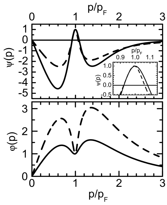
Figure 1: Shape factor $\psi(p)$ (top panel) and interaction profile $\varphi(p)$ (bottom panel) versus $p/p_{F}$. The solid (dashed) line corresponds to the case $\beta_{a}=0.1\,p_{F}$, ${\cal V}_{F}N(0)=2.0$ ($\beta_{a}=0.05\,p_{F}$, ${\cal V}_{F}N(0)=2.5$). In both cases $T_{c}\simeq 10^{-3}\epsilon^{0}_{F}$. The inset depicts the behavior of the shape factor in the vicinity of the Fermi surface.

The lower panel of Fig. 1 shows $\varphi(p)\equiv{\cal V}(p,p_{F})/{\cal V}(p_{F},p_{F})$, the interaction profile in the $P$-pairing channel. This function has the shape of a wide hump, with a narrow dip at $p=p_{F}$. The $P$-wave shape factor $\psi(p)$, which vanishes for $p\to 0$, is shown in the upper panel. It exhibits a narrow, sharp peak at the Fermi surface that creates two nodes, one on either side of the Fermi surface and lying very close to $p_{F}$.

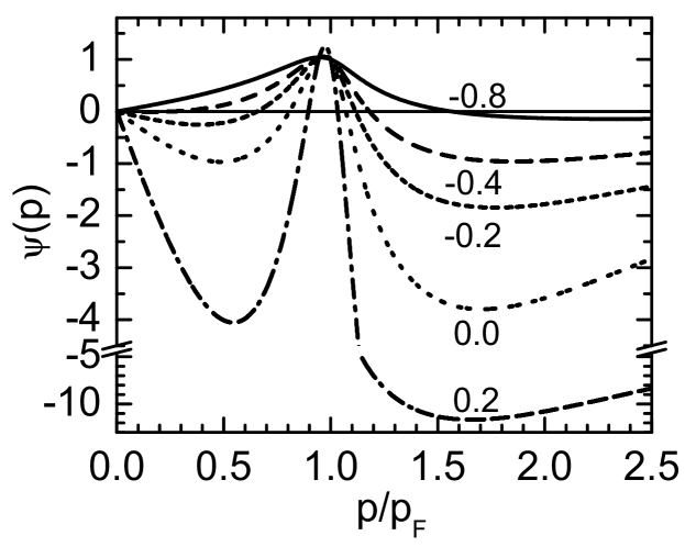
Figure 2: $P$-pairing shape factor $\psi(p)$ as a function of $p/p_{F}$. The interaction form (32) is assumed, with $V_{a}N(0)=1$, $\beta_{a}/p_{F}=0.1$, $\beta_{r}/p_{F}=2$, and five different values of the strength parameter $V_{r}$ of the repulsive component. The curves are labelled with the corresponding values of the $P$-wave coupling parameter $v_{F}\equiv{\cal V}_{F}N(0)$.

Now we address the question: how does the number of nodes in the shape factor $\psi(p)$ change as ${\cal V}_{F}$ is varied while holding $V_{a}$ fixed? Evidently, if the repulsion is weak, then the shape factor $\psi(p)$ has no nodes at all. However, if the repulsion begins to rise, such that ${\cal V}_{F}$ attains a critical value ${\cal V}_{1F}$, the first node of $\psi(p)$ emerges at some momentum $p_{0}>p_{F}$. Whether the sign of ${\cal V}_{1F}$ remains negative or already becomes positive will depend on the particular form of the pairing interaction and on the input parameters that specify it. With further increase of ${\cal V}_{F}$, the nodal location $p_{0}$ moves toward the Fermi surface from the outside. However, the destination $p_{0}=p_{F}$ turns out to be unattainable [18].

Meanwhile, as ${\cal V}_{F}$ continues to increase and reaches a critical value ${\cal V}_{2F}$, a second node of $\psi(p)$ emerges at some momentum value below $p_{F}$ and moves rapidly toward the Fermi surface from the inside. As we shall see, the two nodes crowd the Fermi surface more and more tightly as ${\cal V}$ rises higher and higher above the threshold ${\cal V}_{2F}$.

Fig. 2 presents results from numerical calculations of the shape factor $\psi(p)$, based again on the the interaction ${\cal V}$ defined in Eq. (32). However, we now choose $V_{a}N(0)=-1.0$ and illustrate the sensitivity of the results to the potential parameters. The choice $\beta_{a}=0.1p_{F}$ is maintained, but $\beta_{r}$ is increased to $2p_{F}$. From this figure, we may infer that the first node of $\psi(p)$ emerges at some large momentum $p\sim\infty$ when $v_{F}\equiv{\cal V}_{1F}N(0)\simeq-1.0$. Also, it is important to note that in contrast to the situation found in Fig. 1, the second node of the shape factor now comes on the scene while ${\cal V}_{F}$ is still negative, with a value ${\cal V}_{2F}N(0)\simeq-0.3$. Thus, we conclude that the sign of the critical value of the parameter ${\cal V}_{F}$ for emergence of the second node of $\psi(p)$ depends nontrivially on the specific choice of input parameters.

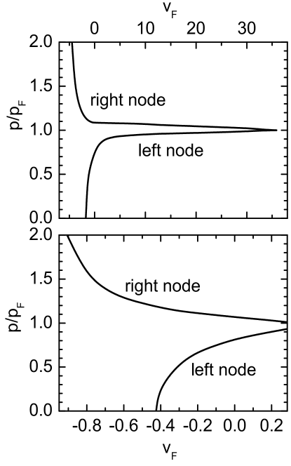
Figure 3: Trajectories of the pair of nodes that appear in the $P$-pairing shape function $\psi(p)$ of Fig. 1 (top panel) and Fig. 2 (bottom panel), versus the $P$-wave coupling parameter $v_{F}$.

In Fig. 3, we display the trajectories of the nodes of the shape factor $\psi(p)$ under variation of the key parameter ${\cal V}_{F}$, with the same parameter setups as in Figs. 1 and 2. The two nodes rapidly approach the Fermi surface from opposite sides as $v_{F}={\cal V}_{F}N(0)$ tends to toward a critical value $v_{Fc}$. (Once again, as seen, this critical value depend crucially on the specifics of the input potential parameters.)

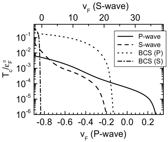
Figure 4: Critical temperature $T_{c}$ (in units of $\varepsilon_{F}^{0}=p_{F}^{2}/2M$), plotted against $P$-wave (bottom axis) and $S$-wave (top axis) coupling parameters $v_{F}\equiv{\cal V}_{F}N(0)$, for a model interaction of form (32). The solid curve corresponds to $P$-pairing, and the dashed curve, to $S$-pairing. For comparison we show the BCS estimate (35) of $T_{c}$ for $P$-pairing (dotted curve) and for $S$-pairing (dot-dashed curve).

5 Discussion

A complete theory of superfluid ³He must give a quantitative description of its kinetic phenomena as well as its thermodynamic properties. Necessarily, then, such a theory takes explicit account of the damping of single-particle excitations – as, for example in the weak-coupling-plus (WCP) theory [7, 10, 11, 12]. By virtue of the scope of WCP theory, its phenomenological character entails the introduction of a large number of adjustable parameters, which inevitably complicates the interpretation of new experimental results. In contrast to this approach, our concentration on the thermodynamics of superfluid ³He has allowed us to retain the conceptually simpler Landau picture [1]. In essence, this picture stems from the basic statement, or assumption, that the ground-state energy and other thermodynamic quantities are functionals of the quasiparticle momentum distribution $n(p)$. Seemingly innocuous at first sight, the Landau assumption leads rather directly to the determination of this distribution function, which can be expressed in the same form as the Fermi-Dirac momentum distribution, $n(p)=[1+\exp(\epsilon(p)/T)]^{-1}$. There is an important distinction, however, namely that the Landau quasiparticle spectrum $\epsilon_{\mbox{\scriptsize FL}}(p)=p_{F}(p-p_{F})/M^{*}$ differs from the single-particle spectrum of the ideal Fermi gas, since it involves an effective mass $M^{*}$ different from the bare mass $M$. In fact, this formula for $\epsilon_{\mbox{\scriptsize FL}}$ is the most vulnerable element of Landau theory as traditionally practiced. The spectrum $\epsilon_{\mbox{\scriptsize FL}}(p)$ ceases to be meaningful close to the quantum critical point (QCP) where the effective mass $M^{*}$ diverges. To rectify the theory, one must take into account contributions to $\epsilon(p)$ from terms $\sim(p-p_{F})^{3}$, as established in Ref. [13]. This extension of the Landau quasiparticle picture alters the standard Fermi-liquid formulas, with the implication that in the vicinity of the QCP, (so-called) non-Fermi-liquid behavior is predicted within the Fermi-liquid approach itself.

A parallel situation may arise in superfluid Fermi liquids. Non-BCS behavior can be deduced within the standard BCS approach provided a well-pronounced momentum dependence of the gap function $\Delta(p)$, driven by the momentum dependence of the pairing interaction, is properly incorporated. In liquid ³He, the bare atom-atom interaction, as modelled in Ref. [20] by a local two-body potential function in coordinate space, contains a huge repulsive core of radius $r_{c}\simeq 2.5\,\AA$, surrounded by an attractive, long-range (power-law) van der Waals component. The properties of this in-vacuum interaction are presumably mirrored by an in-medium pairing interaction ${\cal V}$ consisting of a local repulsive component at short distance and a longer-range attractive term [16, 23]. From the perspective offered and supported in this paper, the existence of $P$-wave superfluidity in liquid ³He implies the presence of an attractive component $V_{a}$ of the effective pairing interaction ${\cal V}$ strong enough to outperform the repulsion at distances slightly exceeding the average distance $r_{0}$ between particles. On the other hand, at large pressures, the repulsive part $V_{r}$ of the effective interaction increases rapidly with the density $\rho$. Indirect evidence for the latter inference is seen in the fast growth of the sound velocity at pressures $P\simeq P_{\rm max}$.

Let us suppose that the parameter ${\cal V}(p_{F},p_{F})$ has already turned positive at pressures close to $P_{\rm max}$, resulting in the appearance of two nodes in the shape factor $\psi(p)$ of the gap function that hold the Fermi surface in a “vice-like grip.” Furthermore, to facilitate the analysis, let us assume that these nodes are situated symmetrically with respect to the Fermi surface on either side of it, so that their locations may be specified by a single parameter. The plots of $\psi(p)$ obtained for models based on the pairing interaction (32) indicate that this assumption is not unreasonable (see Figs. 1 and 2). It becomes more reasonable when long-wavelength spin fluctuations, analogous to the mediating phonons of conventional superconductors, dominate in the attractive part of ${\cal V}$, since in this case the induced pairing interaction is symmetrical with respect to departures of the quasiparticle momenta from the Fermi surface.

Numerical analysis shows that the dominant contributions to the integral $I_{1}(0)$ of Eq. (12) come from the interval $[-\epsilon_{0},\epsilon_{0}]$. Upon neglecting the contributions from the remainder of momentum space and introducing a new integration variable $x=\epsilon/\epsilon_{0}$, the integral (12) takes the form

$$I_{1}(0)=(\Delta^{2}(0)/\epsilon_{0}^{2})K(0)\ ,$$ (33)

where

$$K(0)=2\int\limits_{0}^{1}{1-\psi^{4}(x)\over x\sqrt{x^{2}+\Delta^{2}(0)/\epsilon^{2}_{0}}\left(x+\sqrt{x^{2}+\Delta^{2}(0)/\epsilon^{2}_{0}}\right)}dx\ .$$ (34)

It should be emphasized that deviations of the ratios $r_{\Delta}$ and $r_{C}$ from their BCS values proportional to the ratio $\Delta^{2}(0)/\epsilon_{0}^{2}$ will depend crucially on the structure the shape factor $\psi(x)$ in the interval $0<x<1$. To support this statement, we calculate the value of the integral (34) for two phenomenological shape factors: (i) $\psi(x)=1-x^{2}$ and (ii) $\psi(x)=(1-x^{2})^{\alpha}$. In the latter case we take $\alpha=1.6$, a value that provides an adequate fit of $\psi(x)$ as given in Fig. 1. Calculation of the integral in (34) yields $K(0)=6$ in the first case and $K(0)=50$ in the second.

We may attempt to narrow the uncertainty in the value of the parameter $\epsilon_{0}$, based on the observation that in the normal state at pressures $P$ close to the melting point, the experimental spin susceptibility $\chi(T)$ coincides with the Curie susceptibility $\chi_{C}(T)=\rho/T$ at $T\geq 0.4$ K. This finding implies that at $P\simeq P_{\rm max}$, the bandwidth $\Omega=\epsilon(p_{F})-\epsilon(p=0)$ may be estimated as 0.2–0.3 K. We then suggest that for $P\simeq P_{\rm max}$, the value of $\epsilon_{0}$, which must be significantly less than $\Omega$, lies in the interval 0.05–0.1 K. Inserting this estimate into Eq. (33), along with the two values obtained for $K(0)$, one obtains a range of values for the deviation of $r_{\Delta}$ from the BCS value in the interval 1%-50%.

In Fig. 4 we present results from calculations of the critical temperature $T_{c}$ for $P$-pairing and $S$-pairing as a functions of the coupling parameter $v_{F}={\cal V}_{F}N(0)$. Once again, a pairing interaction of form (32) is assumed to have the same set of parameters as in Fig. 2. Here we also take the opportunity to highlight the problematic nature of the standard BCS formula commonly used to estimate the critical temperature for pair condensation in fermionic systems,

$$T_{c}={2\gamma\over\pi}\Omega_{D}\exp\left(-{2\over\lambda N(0)}\right)\ ,$$ (35)

wherein $N(0)=p_{F}M^{*}/\pi^{2}$ is the density of states, $\Omega_{D}$ is the Debye frequency, and $\lambda$ is the coupling constant, usually identified with $-{\cal V}_{F}$. Fig. 4 compares critical temperatures obtained with this formula (curves labelled BCS(P) and BCS(S)) with those determined by direct solution of the gap equation taking full account of the shape dependence of the gap function. Evidently, the estimate (35) is irrelevant if ${\cal V}_{F}>0$, so meaningful comparisons can only be made for $v_{F}>0$. It is seen that the formula (35) already begins to fail well before ${\cal V}_{F}$ changes its sign. In general, then, the domain where superfluidity exists is wider than that where ${\cal V}_{F}$ is negative, a fact long appreciated within the theory of nucleonic superfluids (see Refs. [21, 22, 18] and works cited therein). In light of this conclusion, the findings of Kuchenhoff and Wölfle [24] on the occurrence of superconductivity in the dilute electron gas bear re-examination, since these authors determined the extent of the superconducting phase from the condition ${\cal V}_{F}<0$. Referring once more to Fig. 4, we may also note that $P$-pairing wins the energetic contest with $S$-pairing when the key parameter ${\cal V}_{F}$ takes on positive values.

A similar situation may exist for unconventional $D$-pairing in heavy-fermion metals. A conspicuous example is CeCoIn₅, for which the antiferromagnetic state lies well above the ground paramagnetic state, implying that antiferromagnetic fluctuations are irrelevant to pairing in the ground state. In principle, there are several sources for attraction in the pairing interaction ${\cal V}$; these include optical phonons and density fluctuations associated with the proximity to a critical density where electron liquid ceases to be homogeneous [25]. We argue that the attractive part of ${\cal V}$ changes insignificantly in switching from $S$- to $D$-pairing, while the repulsive part drops substantially. Thus, in certain heavy-fermion metals, unconventional $D$-pairing may win the contest with conventional $S$-pairing if there is sufficient weakening of the repulsion in the $D$-wave channel relative to that in the $S$-wave channel.

In conclusion, we have analyzed the anomalous behavior of certain thermodynamic properties of superfluid phases of ³He in the framework of the Landau quasiparticle picture. Principally, this behavior consists of departures of experimental results from two famous BCS relations, one quantifying the ratio of the pairing gap at zero temperature to the critical temperature, and the other, the ratio, at this temperature, of the difference between normal and superfluid specific heats to the normal specific heat, We have proposed and demonstrated that, within the quasiparticle picture, these discrepancies may be traced to the emergence of a pair nodes in the gap function lying close to and on opposite sides of the Fermi surface. We have found that a quantitative explanation of the anomalies requires only two phenomenological parameters, one specifying the location of the nodes of the gap function, and the other setting the scale of strong-coupling corrections. Finally, it should be noted that our phenomenological theory has little in common with the (likewise phenomenological) weak-coupling-plus theory of Refs. [7, 10, 11, 12], in which the momentum dependence of the gap function is completely ignored.

References

- [1] L. D. Landau, JETP 30, 1058 (1956).
- [2] I. A. Todoshchenko, H. Alles, A. Babkin, A. Ya. Parshin, and V. Tsepelin, J. Low Temp. Phys. 126, 1449 (2002).
- [3] D. S. Greywall, Phys. Rev. B 33, 7520 (1986).
- [4] P. W. Anderson and W. F. Brinkman, Phys. Rev. Lett. 30, 1108 (1973).
- [5] N. D. Mermin and G. Stare, Phys. Rev. Lett. 30, 1135 (1973).
- [6] W. F. Brinkman and P. W. Anderson, Phys. Rev. A 8, 2732 (1973).
- [7] W. F. Brinkman, J. W. Serene, and P. W. Anderson, Phys. Rev. A 10, 2386 (1974).
- [8] A. J. Leggett, Rev. Mod. Phys. 47, 331 (1975).
- [9] D. Vollhardt and P. Wölfle, The Superfluid Phases of Helium-3 (Taylor & Francis, London, 1990).
- [10] D. Rainer and J. W. Serene, Phys. Rev. B 13, 4745 (1976).
- [11] J. W. Serene and D. Rainer, Phys. Rev. B 17, 2901 (1978); J. Low Temp. Phys. 34, 589 (1979).
- [12] J. A. Sauls and J. W. Serene, Phys. Rev. B 24, 183 (1981).
- [13] J. W. Clark, V. A. Khodel, and M. V. Zverev, Phys. Rev. B 71, 012401 (2005).
- [14] C. H. Aldrich, III, and D. Pines, J. Low Temp. Phys. 32, 689 (1978).
- [15] K. Levin and O. Valls, Phys. Rev. B 20, 105, 120 (1979).
- [16] K. Bedell and D. Pines, Phys. Rev. Lett. 45, 39 (1980).
- [17] M. Pfitzner and P. Wölfle, Phys. Rev. B 35, 4699 (1987).
- [18] V. A. Khodel, V. V. Khodel, and J. W. Clark, Nucl. Phys. A 598, 390 (1996).
- [19] E. M. Lifshitz and L. P. Pitaevskii, Statistical Physics, (Nauka, Moscow, 1978; Pergamon, New York, 1980), p. 193.
- [20] R. A. Aziz, V. P. S. Nain, J. S. Carley, W. L. Taylor, and G. T. McConville, J. Chem. Phys. 70, 4332 (1979).
- [21] E. Krotscheck and J. W. Clark, Nucl. Phys. A333, 77 (1980).
- [22] J. M. C. Chen, J. W. Clark, R. D. Dáve, and V. V. Khodel, Nucl. Phys. A555, 59 (1993).
- [23] L. P. Pitaevskii, JETP 37, 577 (1959); ibid. 37, 1794 (1959).
- [24] S. Kuchenhoff and P. Wölfle, Phys. Rev. B 38, 935 (1988).
- [25] V. V. Borisov, M. V. Zverev, JETP Lett. 81, 503 (2005).