Counting statistics of coherent population trapping in quantum dots

Abstract

Destructive interference of single-electron tunneling between three quantum dots can trap an electron in a coherent superposition of charge on two of the dots. Coupling to external charges causes decoherence of this superposition, and in the presence of a large bias voltage each decoherence event transfers a certain number of electrons through the device. We calculate the counting statistics of the transferred charges, finding a crossover from sub-Poissonian to super-Poissonian statistics with increasing ratio of tunnel and decoherence rates.

I Introduction

The phenomenon of coherent population trapping, originating from quantum optics, has recently been recognized as a useful and interesting concept in the electronic context as well.Bra04 ; Sie04 An all-electronic implementation, proposed in Ref. Mic06, , is based on destructive interference of single-electron tunneling between three quantum dots (see Fig. 1). The trapped state is a coherent superposition of the electronic charge in two of these quantum dots, so it is destabilized as a result of decoherence by coupling to external charges. In the limit of weak decoherence one electron is transferred on average through the device for each decoherence event.

In an experimental breakthrough,Gus06 ; Gus06-2 Gustavsson et al. have now reported real-time detection of single-electron tunneling, obtaining the full statistics of the number of transferred charges in a given time interval. The first two moments of the counting statistics give the mean current and the noise power, and higher moments further specify the correlations between the tunneling electrons.Bla00 This recent development provides a motivation to investigate the counting statistics of coherent population trapping, going beyond the first moment studied in Ref. Mic06, .

Since the statistics of the decoherence events is Poissonian, one might surmise that the charge counting statistics would be Poissonian as well. In contrast, we find that charges are transferred in bunches instead of independently as in a Poisson process. The Fano factor (ratio of noise power and mean current) is three times the Poisson value in the limit of weak decoherence. We identify the physical origin of this super-Poissonian noise in the alternation of two decay processes (tunnel events and decoherence events) with very different time scales—in accord with the general theory of Belzig.Bel05 For comparable tunnel and decoherence rates the noise becomes sub-Poissonian, while the Poisson distribution is approached for strong decoherence.

The analysis of Ref. Mic06, was based on the Lindblad master equation for electron transport,Naz93 ; Gur98 which determines only the average number of transferred charges. The full counting statistics can be obtained by an extension of the master equation due to Bagrets and NazarovBag03 (without phase coherence) and to Kießlich et al.Kie06 (with phase coherence). In spite of the added complexity, we have found analytical solutions for the second moment at any decoherence rate and for the full distribution in the limit of weak or strong decoherence.

II Model

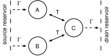
Figure 1: Three quantum dots connected to a source and a drain reservoir. Reversible transitions (rate $T$) and irreversible transitions (rate $\Gamma$) are indicated by arrows.

The system under consideration, studied in Ref. Mic06, , is depicted schematically in Fig. 1. It consists of three tunnel-coupled quantum dots connected to two electron reservoirs. In the limit of large bias voltage, which we consider here, electron tunneling from the source reservoir into the dots and from the dots into the drain reservoir is irreversible. We assume that a single level in each dot lies within range of the bias voltage. We also assume that due to Coulomb blockade there can be at most one electron in total in the three dots. The basis states, therefore, consist of the state $\left|0\right>$ in which all dots are empty, and the states $\left|A\right>$, $\left|B\right>$, and $\left|C\right>$ in which one electron occupies one of the dots.

The time evolution of the density matrix $\rho$ for the system is given by the Lindblad-type master equation,Naz93 ; Gur98

$$\frac{\mathrm{d}\rho}{\mathrm{d}t}=-i[H,\rho]\\ +\sum_{X=A,B,C,\phi_{A},\phi_{B},\phi_{C}}\big{(}L_{X}\rho L^{\dagger}_{X}-\tfrac{1}{2}L^{\dagger}_{X}L_{X}\rho-\tfrac{1}{2}\rho L^{\dagger}_{X}L_{X}\big{)}.$$ (1)

The Hamiltonian

$$H=T\left|C\right>\left<A\right|+T\left|C\right>\left<B\right|+\mathrm{H.c.}$$ (2)

is responsible for reversible tunneling between the dots, with tunnel rate $T$. For simplicity, we assume that the three energy levels in dots $A$, $B$, and $C$ are degenerate and that the two tunnel rates from $A$ to $C$ and from $B$ to $C$ are the same. The quantum jump operators

$$L_{A}=\sqrt{\Gamma}\left|A\right>\left<0\right|,\quad L_{B}=\sqrt{\Gamma}\left|B\right>\left<0\right|,$$

$$L_{C}=\sqrt{\Gamma}\left|0\right>\left<C\right|,$$ (3)

model irreversible tunneling out of and into the reservoirs, with a rate $\Gamma$ (which we again take the same for each dot). Finally, the quantum jump operators

$$L_{\phi_{X}}=\sqrt{\Gamma_{\phi}}\left|X\right>\left<X\right|,\quad X=A,B,C,$$ (4)

model decoherence due to charge noise with a rate $\Gamma_{\phi}$.

As a basis for the the density matrix we use the four states

$$\left|e_{0}\right>=2^{-1/2}(\left|A\right>-\left|B\right>),$$

$$\left|e_{1}\right>=2^{-1/2}(\left|A\right>+\left|B\right>),$$

$$\left|e_{2}\right>=\left|C\right>,\quad\left|e_{3}\right>=\left|0\right>.$$ (5)

If the initial state is $\left|0\right>\left<0\right|$ most of the coefficients of $\rho$ remain zero. We collect the five non-zero real variables in a vector

$$v=(\rho_{00},\rho_{11},\rho_{22},\rho_{33},\mathrm{Im}\,\rho_{02})^{\mathrm{T}},$$ (6)

whose time evolution can be expressed as

$$\mathrm{d}v/\mathrm{d}t=Xv,$$ (7)

$$X=\left(\begin{array}[]{ccccc}\Gamma_{\phi}/2&-\Gamma_{\phi}/2&0&\Gamma&0\\ -\Gamma_{\phi}/2&\Gamma_{\phi}/2&0&\Gamma&-2^{3/2}T\\ 0&0&-\Gamma&0&2^{3/2}T\\ 0&0&\Gamma&-2\Gamma&0\\ 2^{1/2}T&0&-2^{1/2}T&0&-\Gamma/2-\Gamma_{\phi}\end{array}\right).$$ (13)

It is our goal to determine the full counting statistics, being the probability distribution $P(n)$ of the number of transferred charges in time $t$. Irrelevant transients are removed by taking the limit $t\to\infty$. The associated cumulant generating function $F(\chi)$ is related to $P(n)$ by

$$\exp[-F(\chi)]=\sum_{n=0}^{\infty}P(n)\exp(in\chi).$$ (14)

From the cumulants

$$C_{k}=-(-i\partial_{\chi})^{k}F(\chi)|_{\chi=0}$$ (15)

we obtain the average current $I=eC_{1}/t$ and the zero-frequency noise $S=2e^{2}C_{2}/t$, both in the limit $t\to\infty$. The Fano factor is defined as $\alpha=C_{2}/C_{1}$.

As described in Refs. Bag03, and Kie06, , in order to calculate $F(\chi)$ one multiplies coefficients of the rate matrix $X$ which are associated with tunneling into one of the reservoirs (the right one in our case), by counting factors $\mathrm{e}^{i\chi}$. This leads to the $\chi$-dependent rate matrix

$$L(\chi)=\left(\begin{array}[]{ccccc}\Gamma_{\phi}/2&-\Gamma_{\phi}/2&0&\Gamma&0\\ -\Gamma_{\phi}/2&\Gamma_{\phi}/2&0&\Gamma&-2^{3/2}T\\ 0&0&-\Gamma&0&2^{3/2}T\\ 0&0&\Gamma\mathrm{e}^{i\chi}&-2\Gamma&0\\ 2^{1/2}T&0&-2^{1/2}T&0&-\Gamma/2-\Gamma_{\phi}\end{array}\right).$$ (16)

The cumulant generating function for $t\to\infty$ can then be obtained from the eigenvalue $\Lambda_{\mathrm{min}}(\chi)$ of $L(\chi)$ with the smallest absolute real part,Bag03 ; Kie06

$$F(\chi)=-t\Lambda_{\mathrm{min}}^{(\chi)}.$$ (17)

III Results

III.1 Fano factor

Low order cumulants can be calculated by perturbation theory in the counting parameter $\chi$. The calculation in outlined in App. A. For the average current we find

$$I=\frac{4e\Gamma T^{2}}{\Gamma^{2}+14T^{2}+2\Gamma\Gamma_{\phi}(1+2T^{2}/\Gamma_{\phi}^{2})},$$ (18)

in agreement with Ref. Mic06, . By calculating the noise power and dividing by the mean current we obtain the Fano factor

$$\alpha = \Big{[}\Gamma^{4}+148T^{4}+4\Gamma^{2}(\Gamma_{\phi}^{2}+4T^{2}+12T^{4}/\Gamma_{\phi}^{2})+$$ (19)

$$(16T^{2}+2\Gamma^{2})\beta\Big{]}\Big{[}\Gamma^{2}+14T^{2}+\beta\Big{]}^{-2},$$

$$\beta = 2\Gamma\Gamma_{\phi}(1+2T^{2}/\Gamma_{\phi}^{2}).$$ (20)

In Fig. 2 the Fano factor has been plotted as a function of $\Gamma_{\Phi}/T$ for three different values of $\Gamma/T$. The dependence of the Fano factor on the decoherence rate is nonmonotonic, crossing over from super-Poissonian ($\alpha>1$) to Poissonian ($\alpha=1$) via a region of sub-Poissonian noise ($\alpha<1$). To obtain a better understanding of this behavior, we study separately the regions of weak and strong decoherence.

Figure 2: Dependence of the Fano factor $\alpha$ on the normalized decoherence rate $\Gamma_{\phi}/T$ for three values of $\Gamma/T$.

III.2 Weak decoherence

For decoherence rate $\Gamma_{\phi}\ll\Gamma,T$ we have the limiting behavior

$$I\to e\Gamma_{\phi},\quad\alpha\to 3-\Gamma_{\phi}\left(\frac{17}{\Gamma}+\frac{\Gamma}{T^{2}}\right).$$ (21)

Hence one charge is transferred on average per decoherence event, but the Fano factor is three times the value for independent charge transfers.

There exists a simple physical explanation for this behavior. For zero decoherence the system becomes trapped in the state $\left|e_{0}\right>$. The system is untrapped by “decoherence events”, which occur randomly at the rate $\Gamma_{\phi}$ according to Poisson statistics. If $\Gamma_{\phi}$ is sufficiently small there is enough time for the system to decay into the trapped state between two subsequent events, so they can be viewed as independent. The super-Poissonian statistics appears because a single decoherence event can trigger the transfer of more than a single charge.

The probability of $n$ electrons being transferred in total as a consequence of one decoherence event is

$$R^{1}(n)=\frac{1}{2^{n+1}},$$ (22)

since a decoherence event projects the trapped state $\left|e_{0}\right>$ onto itself or onto $\left|e_{1}\right>$ with equal probabilities $1/2$ and each electron subsequently entering the dots has a 50% chance of getting trapped in the state $\left|e_{0}\right>$.

The number of electrons which have been transferred due to exactly $k$ decoherence events has distribution $R^{k}(n)$, the $(k-1)$th convolution of $R^{1}(n)$ with itself. We get

$$R^{k}(n) = \frac{1}{2^{n+k}}\sum_{i_{0}=0}^{n}\sum_{i_{1}=0}^{i_{0}}\cdots\sum_{i_{k-2}=0}^{i_{k-3}}1$$ (23)

$$= \frac{1}{2^{n+k}}\binom{n+k-1}{n}.$$

By definition,

$$R^{0}(n)=\delta_{n,0}=\left\{\begin{array}[]{c}1\\ 0\end{array}\,\mathrm{for}\,\begin{array}[]{l}n=0\\ n>0\end{array}\right.,$$ (24)

being the distribution of the transferred charges after no decoherence events have occurred.

The decoherence events in a time $t$ have a Poisson distribution,

$$P_{\mathrm{Poisson}}(k)=\mathrm{e}^{-t\Gamma_{\phi}}(t\Gamma_{\phi})^{k}/k!.$$ (25)

Combining with Eq. (23) we find the probability that $n$ electrons have been transferred during a time $t$,

$$P(n) = \sum_{k=0}^{\infty}P_{\mathrm{Poisson}}(k)R^{k}(n)$$

$$= \sum_{k=1}^{\infty}\frac{\mathrm{e}^{-t\Gamma_{\phi}}(t\Gamma_{\phi})^{k}}{2^{n+k}k!}\binom{n+k-1}{n}+\mathrm{e}^{-t\Gamma_{\phi}}\delta_{n,0}.$$

The corresponding cumulant generating function is

$$F(\chi)=t\Gamma_{\phi}-\frac{t\Gamma_{\phi}}{2-\mathrm{e}^{i\chi}},$$ (27)

which gives rise to the cumulants

$$C_{1}=t\Gamma_{\phi},\quad C_{2}=3t\Gamma_{\phi},\quad C_{3}=13t\Gamma_{\phi},$$ (28)

in agreement with Eq. (21).

The probability distribution (27) has been found by Belzig in a different model.Bel05 As shown in that paper, this superposition of Poisson distributions with Fano factor 3 arises generically whenever there are two transport channels with very different transport rates (in our case slow transport via the trapped state $\left|e_{0}\right>$, and fast transport via the untrapped state $\left|e_{1}\right>$).

III.3 Strong decoherence

We show that Poisson statistics of the transferred charges is obtained for strong decoherence. Consider the evolution equation (7) of the system. For $\Gamma_{\phi}\gg\Gamma,T$ the coefficients $X_{00},X_{01},X_{10}$, and $X_{11}$ will ensure that $v_{0}$ is equal to $v_{1}$ after a time which is short compared to the other characteristic times of the system. The trapped and the non-trapped states will be equally populated. Let us therefore define

$$v^{\prime}=(\rho_{00}+\rho_{11},\rho_{22},\rho_{33},\mathrm{Im}\,\rho_{02})^{\mathrm{T}}$$ (29)

and use $\rho_{00}=\rho_{11}=v^{\prime}_{0}/2$. The evolution of $v^{\prime}$ is governed by $\mathrm{d}v^{\prime}/\mathrm{d}t=X^{\prime}v^{\prime}$, with

$$X^{\prime}=\left(\begin{array}[]{cccc}0&0&2\Gamma&-2^{3/2}T\\ 0&-\Gamma&0&2^{3/2}T\\ 0&\Gamma&-2\Gamma&0\\ 2^{-1/2}T&-2^{1/2}T&0&-\Gamma/2-\Gamma_{\phi}\end{array}\right).$$ (30)

The rate matrix $L^{\prime}(\chi)$ is obtained by multiplying $X^{\prime}_{12}$ by the counting factor $\mathrm{e}^{i\chi}$. An analytic expression can be found for the smallest eigenvalue ${\Lambda^{\prime}}_{\mathrm{min}}^{(\chi)}$ of $L^{\prime}(\chi)$, leading to the cumulant generating function

$$F(\chi)=\frac{2T^{2}}{\Gamma_{\phi}}t\left(1-\mathrm{e}^{i\chi}\right)$$ (31)

of a Poisson distribution.

IV Conclusion

In conclusion, we have shown that coherent population trapping in a purely electronic system has a highly nontrivial statistics of transferred charges. Depending on the ratios of decoherence rate and tunnel rates, both super-Poissonian and sub-Poissonian statistics are possible. We have obtained exact analytical solutions for the crossover from sub- to super-Poissonian charge transfer, and have calculated the full distribution in the limits of weak and strong decoherence. We hope that the rich behavior of this simple device will motivate experimental work along the lines of Ref. Gus06, and Gus06-2, .

Appendix A Derivation of the Fano factor

To derive the result (19) for the Fano factor it is sufficient to know the cumulant generating function to second order in $\chi$. The eigenvalues of the rate matrix $L(\chi)$ defined in Eq. (16) have the expansion

$$\lambda=\lambda_{0}+\lambda_{1}\chi+\lambda_{2}\chi^{2}+O(\chi^{3}).$$ (32)

We seek the eigenvalue with the smallest real part in absolute value. That eigenvalue has $\lambda_{0}=0$. We also express the eigenvector $w$ corresponding to $\lambda$ and the matrix itself in a power series in $\chi$:

$$w = w_{0}+w_{1}\chi+w_{2}\chi^{2}+O(\chi^{3}),$$ (33)

$$L = L_{0}+L_{1}\chi+L_{2}\chi^{2}+O(\chi^{3}).$$ (34)

Inserting the above expansions into the eigenvalue equation $Lw=\lambda w$ yields the following relationships of respectively zeroth, first and second order:

$$L_{0}w_{0} = 0,$$ (35)

$$L_{1}w_{0}+L_{0}w_{1} = \lambda_{1}w_{0},$$ (36)

$$L_{2}w_{0}+L_{1}w_{1}+L_{0}w_{2} = \lambda_{2}w_{0}+\lambda_{1}w_{1}.$$ (37)

The coefficients $L_{k}$ are known, while $w_{k}$ and $\lambda_{k}$ remain to be found by solving these equations sequentially. The first two cumulants then follow from

$$C_{1}=-it\lambda_{1},\quad C_{2}=-2t\lambda_{2}.$$ (38)

In an analogue way it is possible to calculate higher cumulants.

References

- (1) T. Brandes, Phys. Rep. 408, 315 (2005) .
- (2) J. Siewert and T. Brandes, Adv. Solid State Phys. 44, 181 (2004).
- (3) B. Michaelis, C. Emary, and C. W. J. Beenakker, Europhys. Lett. 73, 677 (2006).
- (4) S. Gustavsson, R. Leturcq, B. Simovič, R. Schleser, T. Ihn, P. Studerus, K. Ensslin, D. C. Driscoll, and A. C. Gossard, Phys. Rev. Lett. 96, 076605 (2006).
- (5) S. Gustavsson, R. Leturcq, B. Simovič, R. Schleser, P. Studerus, T. Ihn, K. Ensslin, D. C. Driscoll, and A. C. Gossard, cond-mat/0605365.
- (6) Ya. M. Blanter and M. Büttiker, Phys. Rep. 336, 1 (2000).
- (7) W. Belzig, Phys. Rev. B 71, 161301(R) (2005).
- (8) Yu. V. Nazarov, Physica B 189, 57 (1993).
- (9) S. A. Gurvitz, Phys. Rev. B 57, 6602 (1998).
- (10) D. A. Bagrets and Yu. V. Nazarov, Phys. Rev. B 67, 085316 (2003).
- (11) G. Kießlich, P. Samuelsson, A. Wacker, and E. Schöll, Phys. Rev. B 73, 033312 (2006).