Computation of entropy increase for Lorentz gas and hard disks

Laboratoire Matière et Systèmes Complexes (MSC)

UMR 7057 CNRS et Université Paris 7- Denis Diderot

Case 7020, Tour 24-14.5ème étage, 4, Place Jussieu

75251 Paris Cedex 05 / FRANCE

emails : courbage@ccr.jussieu.fr, saberi@ccr.jussieu.fr

Abstract. Entropy functionals are computed for non-stationary distributions of particles of Lorentz gas and hard disks. The distributions consisting of beams of particles are found to have the largest amount of entropy and entropy increase. The computations show exponentially monotonic increase during initial time of rapid approach to equilibrium. The rate of entropy increase is bounded by sums of positive Lyapounov exponents.

1 Introduction

The H-theorem for dynamical systems describes the approach to equilibrium, the irreversibility and entropy increase for deterministic evolutions. Suppose that a dynamical transformation $T$ on a phase space $X$ has some ”equilibrium” measure $\mu$, invariant under $T$, i.e. $\mu(T^{-1}E)=\mu(E)$ for all measurable subsets $E$ of $X$. Suppose also that there is some mixing type mechanism of the approach to equilibrium for $T$, i.e. there is a sufficiently large family of non-equilibrium measures $\nu$ such that $\nu_{t}(E)=:\nu(T^{-t}E)\rightarrow_{t\rightarrow\infty}\mu(E)$ for all E. Then, the H-theorem means the existence of a negative entropy functional $S(\nu_{t})$ which increases monotonically with $t$ to zero, being attained only for $\nu=\mu$. The existence of such functional in measure-theoretical dynamical systems has been the object of several investigations during last decades see [6]- [9], [11], [14, 15, 18]). Here we study this problem for the Lorentz gas and hard disks. The dynamical and stochastic properties of the Lorentz gas in two dimensions which we consider here was investigated by Sinaï and Bunimovich as an ergodic dynamical system [16, 4, 5]. Other transport properties have been also studied numerically (see [12], [19]). This is a system of non interacting particles moving with constant velocity and being elastically reflected from periodically distributed scatterers. The scatterers are fixed disks. On account of the absence of interactions between particles the system is reduced to the motion of one billiard ball. We shall investigate the entropy increase under the effect of collisions of the particles with the obstacles. For this purpose, we consider the map $T$ which associates to an ingoing state of a colliding particle the next ingoing colliding state. The particle moves on an infinite plane, periodically divided into squares of side $D$ called ”cells”, on the center of which are fixed the scatterers of radius $a$ ( Fig. 1). The ingoing colliding state is described by an ingoing unitary velocity arrow at some point of the disk. To a colliding arrow $\textbf{V}_{1}(P_{1})$ at point $P_{1}$ on the boundary of the disk the map associates the next colliding arrow $\textbf{V}_{2}(P_{2})$ according to elastic reflection law. Thus, the collision map does not take into account the free evolution between successive collisions.

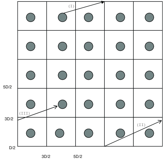
Figure 1: The motion of the particle on a toric billiard.

Let $\nu$ be a non-equilibrium measure, which means that $\nu$ is a non invariant measure approaching the equilibrium $\mu$ in the future. It is mathematically possible to define a non-equilibrium entropy for a family of such measures, using conditional expectations (i.e. a generalized averaging) relatively to the some remarkable partitions, namely the contracting fibers of the hyperbolic dynamics [6]. However, in our numerical simulations some given finite precision is needed, so that we consider partitions into cells with positive $\mu$-measure. Here, we use slightly similar entropy functionals. Starting from the non-equilibrium initial distribution $\nu$, and denoting by $\mathcal{P}$ such partition formed by cells ($\mathcal{P}_{1}$,$\mathcal{P}_{2}$, …, $\mathcal{P}_{n}$) and by $\nu_{t}(\mathcal{P}_{i})=\nu\circ T^{-t}(\mathcal{P}_{i})$, the probability at time $t$ for the system to be in the cell $\mathcal{P}_{i}$ and such that $\nu(\mathcal{P}_{i})\neq\mu(\mathcal{P}_{i})$ for some $i$, the approach to equilibrium implies that $\nu_{t}(\mathcal{P}_{i})\rightarrow\mu(\mathcal{P}_{i})$ as $t\rightarrow\infty$ for any $i$. The entropy functional will be defined by:

$$\mathcal{S}(t,\nu,\mathcal{P})=-\sum_{i=1}^{N}\nu_{t}(\mathcal{P}_{i})\ln(\frac{\nu_{t}(\mathcal{P}_{i})}{\mu(\mathcal{P}_{i})}):=-\mathcal{H}(t,\nu,\mathcal{P})$$ (1.1)

which we simply denote here after $\mathcal{S}(t)$. The H-functional (1.1) is maximal when the initial distribution is concentrated on only one cell and minimal if and only if $\nu_{t}(\mathcal{P}_{i})=\mu(\mathcal{P}_{i}),\forall i$. These properties are shown straightforwardly.
This formula describes the relative entropy of the non-equilibrium measure $\nu_{t}$ with respect to $\mu$ for the observation associated to $\mathcal{P}$. It coincides with the information theoretical concept of relative entropy of a probability vector $(p_{i})$ with respect to another probability vector $(q_{i})$ defined as follows: $-\ln p_{i}$ being the information of the $i^{\mathrm{th}}$ issue under the first distribution, $-\sum_{i}p_{i}\ln(\frac{p_{i}}{q_{i}})$, is equal to the average uncertainty gain of the experience $(p_{i})$ relatively to $(q_{i})$.
A condition under which formula (1.1) shows a monotonic increase with respect to $t$ is that the process $\nu_{t}(\mathcal{P}_{i})=\nu\circ T^{-t}(\mathcal{P}_{i})$ verifies the Chapman-Kolmogorov equation valid for Markov chains and other infinite memory chains. For a dynamical system, this condition is hardly verified for given partition $\mathcal{P}$. However, the very rapid mixing leads to a monotonic increase of the above entropy, at least during some initial stage, which can be compared with the relaxation stage in gas theory.
In this paper, we will first compute the entropy increase for some remarkable non-equilibrium distributions over the phase space of the Sinaï billiard. The billiard system is a hyperbolic system (with many singularity lines) and, in order to have a rapid mixing, we will consider initial distributions supported by the expanding fibers. Such initial measures have been used in [6, 9, 18]. For the billiard the expanding fibers are well approximated by particles with parallel arrows velocity. We call this class of initial ensemble beams of particles. We first compute the entropy increase under the collision map for these initial distributions. We will consider finite uniform partitions of the phase space as explained below. The entropy functional will be defined through (1.1). For this purpose, the phase space of the collision map is described using two angles $(\beta,\psi)$, where $\beta$ is the angle between the outer normal at $P$ and the incoming arrows $\textbf{V}(P)$, $\beta\in[0,\frac{\pi}{2}[$, and $\psi\in[0,\pi]$ is the angle between $x$-axis and the outer normal at $P$. Thus, the collision map induces a map: $(\beta_{1},\psi_{1})\rightarrow(\beta_{2},\psi_{2})$ (see Fig.  14) and we shall first use a uniform partition of the $(\beta,\psi)$ space. The computation shows that whatever is the coarsening of these partitions the entropy has the monotonic property in the initial stage. It is clear that, along mixing process, the initial distribution will spread over all cells almost reaching the equilibrium value. Physically, this process is directed by the strong instability, that is expressed by the positive Lyapounov exponent.
We also consider the relation of the rate of increase of the entropy functionals and Lyapounov exponents of the Lorentz gas. Our computation shows that this relation is expressed by an inequality

$$\max(\mathcal{S}(n+1)-\mathcal{S}(n))\equiv\bigtriangleup\mathcal{S}\leq\sum_{\lambda_{i}\geq 0}\lambda_{i}$$ (1.2)

where the ”$\max$” is taken over $n$, which means that the K-S entropy is an upper bound of the rate of increase of this functional.
In section 3, we shall consider another phase space and another partitions associated to spatial extension of the motion of the Lorentz gas. Here the space in which moves a particle is a large torus divided into rectangular cells, in the center of each cell there is one disk. Denoting the total number of cells by $n$ and the number of particles initially distributed in only one region, by $N$, and following them until each executes $t$ collisions with obstacles, we compute the probability that a particle is located in the $i\mathrm{th}$ cell as given by:

$$\rho_{i}(t)=\frac{\mathrm{Number\,of\,particles\,in\,cell\,\emph{i}\,having\,made\,\emph{t}\,collisions}}{N}$$

The equi-distribution of the cells leads to take, as equilibrium measure, $\mu_{i}=\frac{1}{n}$, so that this ”space entropy” is defined by:

$$\mathcal{S}_{sp}(t)=-\sum_{i=1}^{n}\rho_{i}(t)\ln(\rho_{i}(t)n)$$ (1.3)

The maximum of absolute value of this entropy is equal to $-\ln n$. So we normalize as follows:

$${\bf s}_{sp}(t)=\frac{\mathcal{S}_{sp}(t)}{\ln n}$$ (1.4)

In section 4 we shall consider the hard disks systems. We shall compute an entropy functional similar to the space-entropy on extended torus with several cells. The probabilities are defined as for the space entropy in the Lorentz gas. We shall also do some comparisons of the $H$-theorem with the sum of normalized positive Lyapounov exponents.

2 Entropy for collision map

The entropy for the collision map is computed for a beam of $N$ particles on a toric checkerboard with $n$ cells. We start to calculate the entropy, just after all particles have executed the first collision. In this computation, all particles have the same initial velocity and are distributed in a small part of one cell. For each particle we determine the first obstacle and the angles $(\beta_{1},\psi_{1})$ of the velocity incoming vector $\textbf{V}_{1}(P_{1})$ ( see the figures given in the appendix). For a uniform partition $\mathcal{P}$ of the space of the variables $(\beta,\psi)$, the entropy $\mathcal{S}(t)$is computed iteratively just after all particles have executed the $\emph{t}^{\mathrm{th}}$ collision. We use the formula $(\ref{eq1})$ where

$$\mu(\mathcal{P}_{i})=\int_{\beta_{i}}^{\beta_{i+1}}\int_{\psi_{i}}^{\psi_{i+1}}\cos\beta d\beta d\psi$$ (2.5)

Figure 2: Entropy of the collision map versus number of collisions for (a) a beam of 640 particles for a radius a=0.2, neighboring disks centers distance 1 and a partition of $(\beta,\psi)$ space into $25\times 25$ cells, (b) a beam of 512 particles for the obstacles of radius 0.2, neighboring disks centers distance 1 and a partition of $(\beta,\psi)$ space into $9\times 9$ cells.

is the invariant measure [16] of the cell $\mathcal{P}_{i}=[\beta_{i},\beta_{i+1}[\times[\psi_{i},\psi_{i+1}[$ and $\nu_{t}(\mathcal{P}_{i})$ is the probability that a particle is located after t collisions in $\mathcal{P}_{i}$ computed as

$$\frac{\mathrm{Number\,of\,particles\,in\,\mathcal{P}_{i}\,having\,made\,t\,collisions}}{\mathrm{N}}.$$

The velocity after the collision is computed from the following equation:

$$\textbf{V}({P}_{2})=\textbf{V}({P}_{1})-2(\textbf{V}({P}_{1}).\textbf{n})\textbf{n}$$ (2.6)

where n is the normal vector at the collision point. We explain in the appendix the main geometric formula used for this computation. This entropy increase is shown in the Fig. 2 for various partitions and various initial distributions. The absolute value of the entropy of a distribution of particles, that we call its amount of entropy, represents in fact its distance to equilibrium. This is illustrated in the examples of randomly distributed initial velocity of particles having small amount of entropy (see Fig. 3 ) comparatively with beams of particles. It is to be noted that the amount of entropy increase under one collision is remarkably greater for the few first ones (more or less $2$-$4$ collisions) which corresponds to an exponential type increase (Fig. 4).

Figure 3: (a) and (b) are the entropy of the collision map with random initial conditions versus number of collisions for the system of particles of the Fig. 2, respectively.

In order to calculate Lyapounov exponents by using the method of Benettin et al [2], first we calculate the Jacobian matrix in the tangent space of the collision map:

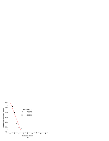
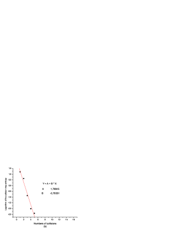
Figure 4: Logarithm of the collision map entropy versus number of collisions for the system of particles of the Fig. 2.

$$\left(\begin{array}[]{cc}\frac{\partial\beta_{2}}{\partial\beta_{1}}&\frac{\partial\beta_{2}}{\partial\alpha_{1}}\\ \\ \frac{\partial\alpha_{2}}{\partial\beta_{1}}&\frac{\partial\alpha_{2}}{\partial\alpha_{1}}\\ \end{array}\right).$$

Now, comparing $\vartriangle\mathcal{S}=\max(\mathcal{S}(t+1)-\mathcal{S}(t))$ (where the ”$\max$” is taken over $t$) with the positive Lyapounov exponent, $\lambda$, of the collision map we verify the inequality:

$$\vartriangle\mathcal{S}<\lambda$$ (2.7)

as shown in Fig. 5, where this exponent is $\sim 3.2$. The maximal entropy increase by collision for the distribution computed in this figure is not far from this value. So it could be conjectured that in some suitable refinement limit, the entropy increase of a beam tends to the positive Lyapounov exponent. The rate of the approach to equilibrium is thus related to the positive Lyapounov exponent. Furthermore, the value of Lyapounov exponent is only dependent of $\frac{D}{a}$, i.e. the ratio of the distance between two successive obstacles over the radius of the obstacle, and its variation is exponential as shown in Fig. 6.

Figure 5: (a) Lyapounov exponent and (b) entropy of the collision map, versus of number of collisions for each particle. We see that the maximum of the entropy increase between two collisions is less than of the value of the Lyapounov exponent.

Figure 6: Lyapounov exponent versus $D/a$.

In order to compare the entropy increase as a function of the collisions with the entropy increase as a function of time, we compute the distribution of mean free time for the first 3 collisions. From time histogram for the first three collisions of this system ( Fig. 7), we see that a great number of particles have the same mean free time. As shown in the table 1, the mean free time vary during the first three or four collisions but after those, for the following collisions, rapidly the system comes near the equilibrium, where we have a constant mean free time approximately.

Collision number	1	2	3	4	5	6	7
Mean free time	1.966	26.174	5.801	3.820	3.611	4.452	4.177
Collision number	8	9	10	11	12	13	14
Mean free time	4.162	4.208	4.212	3.863	4.272	4.051	4.397

Table 1: Mean free time obtained for a beam of 640 particles for a radius a=0.2, neighboring disks centers distance 1 and a partition of $(\beta,\psi)$ space $25\times 25$ cells.

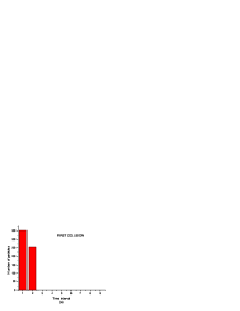
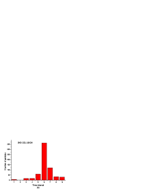
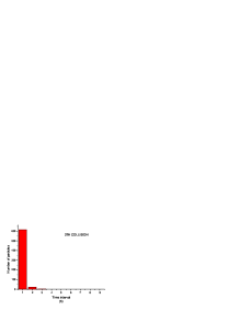
Figure 7: Free time histogram for (a) first, (b) second and (c) third collision.

3 Spatially extended Lorentz gas entropy

The computation of the normalized space entropy equation by using (1.4) versus the number of collisions shows a remarkable exponential increase both for beams and for random initial distributions (Fig. 8). The computation of sum of the two positive Lyapounov exponents of the flow of one particle is equal to $1.046$. Thus, we observe that the inequality between the normalized increase of the density of the space entropy and this sum is verified.

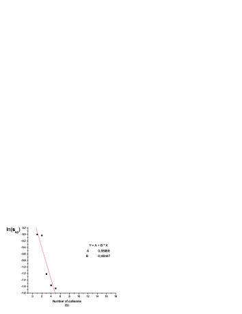
Figure 8: (a) Normalized space entropy of the Lorentz gas versus number of collisions for a beam of 640 particles for obstacles of radius a=0.2, neighboring disks centers distance 1 and a partition of $(x,y)$ space into $25\times 25$ cells, (b) Logarithm of the space entropy versus number of collisions for this system.

4 Hard disks

Considering a uniform space partition of a large toric space we compute the particles densities, $\rho_{i}$, and the normalized space entropy as a function of time by using the equation (1.4). Starting with a distribution of disks with localized positions in some cell and random velocities, we compute binary collisions instants and the trajectories of the hard disks. These instants are determined by checking the distance between particles, after a time interval is passed. The Lyapounov exponents of the flow are calculated by using the Benettin et al. algorithm. The result is shown in the Figs. 9 and  10. These figures show the entropy and logarithm of monotonic part of entropy versus time of the same gas with two distinct densities. The system in the Fig. 10 is more dense than the system in Fig.9, and its entropy increases more rapidly. Fig. 11 is a histogram of the number of collisions, so we see that the number of collisions in a fixed time interval is reduced for large time. From Figs. 9 and 10 we see that the monotonic part of the non-equilibrium entropy is also varying exponentially with respect to time. This shows that the collision is the main ingredient responsible of the entropy increase as described in the Boltzmann equation theory.

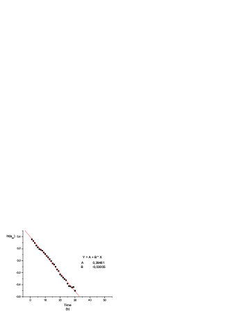
Figure 9: (a) Normalized space entropy and its monotonic part logarithm of the hard disks versus time for the 128 particles for the obstacles of radius a=0.05 which are initially localized in the first cell of $(x,y)$ space with $6\times 6$ cells and a density $\sigma_{1}=0.889$ disks per unit area.

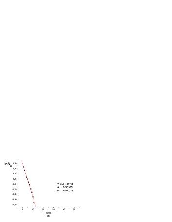
Figure 10: Normalized space entropy and its and its monotonic part logarithm for the same system as Fig. 9, with a density $\sigma_{2}=3.555$ disks per unit area.

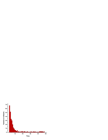
Figure 11: Number of collisions histogram system versus time in Fig. 9.

Figure 12: Normalized spectrum Lyapounov of exponent of system in Fig. 9.

Density	$\frac{1}{N}\sum_{\lambda_{i}>0}(\frac{\lambda_{i}}{\lambda_{max}})$	$\triangle\textbf{s}_{sp}$
3.555	0.367	0.139
0.889	0.294	0.115
0.222	0.239	0.144

Table 2: The data for the hard disks systems of radius, $a=0.05$ and the same initial conditions, with cells $6\times 6$, in terms of the density.

We shall now vary the density $\sigma=\frac{N}{V}$ and compute the characteristic quantities. The graph of the normalized positive Lyapounov exponents spectrum per particle for the same system as in Fig. 9 is shown in Fig.12. The computation of the normalized sums of the positive Lyapounov exponent, $\frac{1}{N}\sum_{\lambda_{i}>0}(\frac{\lambda_{i}}{\lambda_{max}})$, shows that the inequality between maximum entropy increase and the sum of normalized of positive Lyapounov exponents is verified ( Table 2 ).

5 Concluding remarks

The computations of the entropy amount of some given nonequilibrium initial distributions relatively to the equilibrium measure show an exponential type increase for all considered partitions and distributions during initial stage after which the entropy increases slowly and fluctuates near its maximal value. These computations confirm the existence of a relaxation time generally assumed in the derivation of kinetic equations [1] and the origin of the rapid increase of the entropy due to the number of collisions. The dispersive nature of the obstacles is responsible of the exponential mixing type increase. This exponential type increase has been demonstrated for the Sinaï entropy functional [18] in hyperbolic automorphisms of the torus. On the other hand, the relation of the entropy increase to Lyapounov exponents can be understood through Pesin relation and Ruelle inequality. In fact, the rate of entropy increase should be bounded by the Kolmogorov-Sinaï entropy and such bound have been found by Goldstein and Penrose for measure-theoretical dynamical systems under some assumptions [14]. An open question is to characterize the measures reaching the upper bound.

Any entropy functional is not a completely monotonic function of time for any dynamical system. In order to define a completely monotonic entropy functional for a dynamical system some conditions on the dynamics should be imposed. We can first suppose the map $T$ on a phase space $X$ to be a Bernoulli system or, slightly more generally, a $K$-system. This means that there is an invariant measure $\mu$ and some partition $\xi_{0}$ of $X$ such that $T\xi_{0}$ becomes finer than $\xi_{0}$ ( we denote it: $T\xi_{0}\geq\xi_{0}$). Using the notation: $T^{n}\xi_{0}=\xi_{n}$, we obtain a family of increasingly refined partitions, in the sense of the above order of the partitions. Moreover, $\xi_{n}$ tends, as $n\rightarrow\infty$, to the finest partition of $X$ into points, and $\xi_{n}$ tends, as $n\rightarrow-\infty$, to the most coarse partition, into one set of measure $1$ and another set of measure zero. A physical prototype of a Bernoulli and a $K$-system is the above billiard [16, 10]. A geometric prototype of a Bernoulli and a $K$-system is uniformly hyperbolic system with Sinaï invariant measure [17]. A non-equilibrium entropy for a family of initial measures, using conditional expectations relatively to the $\xi_{n}$ partitions was first obtained as an equivalence between the unitary group evolution and a semi-group of contraction operators in the space of square integrable functions $L^{2}(\mu)$ successively for the baker transformation [15], for Bernoulli systems [7] and for K-systems [13]. Its extension to the space of measures in K-systems has been realized in [6]. In differentiable hyperbolic dynamical systems where the fibers of the $\xi_{n}$ partitions are pieces of contracting fibers, the construction of such entropy functional results from a generalized coarse-graining with respect to these contracting fibers, each fiber being a piece of manifold of zero measure.

6 Appendix

6.1 Collision Map

We shall give the formula of the collision map. We consider a particle which undergoes the first collision with the disk of center $\mathrm{O}_{1}$ with velocity $\textbf{V}_{1}(p_{1})$ and the second collision with the disk of center $\mathrm{O}_{2}$ with velocity $\textbf{V}_{1}(p_{2})$. Two cases are possible. First, we consider non-crossing of the centers line as in the Fig. 14. In this figure the angle $\widehat{\mathrm{P_{1}P_{2}}M}$ is $\alpha_{2}-\beta_{2}=-(\alpha_{1}-\beta_{1})$, where $\mathrm{M}$ is such that $\mathrm{MP_{2}}$ is parallel to $\mathrm{O_{1}O_{2}}$. We can write

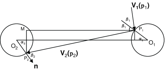
Figure 13: non-crossing Collision.

Figure 14: crossing Collision.

$$\mathrm{P_{1}M}=\mathrm{P_{1}P_{2}}\cos(\beta_{1}-\alpha_{1})=d-a\cos\alpha_{1}-a\cos\alpha_{2}.$$ (6.8)

and

$$\mathrm{P_{2}M}=\mathrm{P_{1}P_{2}}\sin(\beta_{1}-\alpha_{1})=a\sin\alpha_{1}-a\sin\alpha_{2},$$ (6.9)

if we eliminate $\alpha_{2}$ between these equations we arrive at

$$\beta_{2}=\arcsin[\frac{d}{a}\sin(\beta_{1}-\alpha_{1})+\sin\beta_{1}].$$ (6.10)

In crossing case which we present in Fig. 14 we see that the angle $\widehat{\mathrm{P_{2}P_{1}M}}$ is equal to $\alpha_{2}-\beta_{2}=\alpha_{1}-\beta_{1}$, and the length of $\mathrm{P_{2}M}$ is changed to:

$$\mathrm{P_{2}M}=\mathrm{P_{1}P_{2}}\sin(\beta_{1}-\alpha_{1})=a\sin\alpha_{1}+a\sin\alpha_{2},$$ (6.11)

then, we have

$$\beta_{2}=\arcsin[\frac{d}{a}\sin(\beta_{1}-\alpha_{1})-\sin\beta_{1}].$$ (6.12)

To obtain $\beta_{2}$ in the first collision between particle and obstacle Fig. 15 , we take $d=\mathrm{OP_{1}}$, $\beta_{1}=0$ and $\alpha_{1}=\vartheta$ in the collision map.

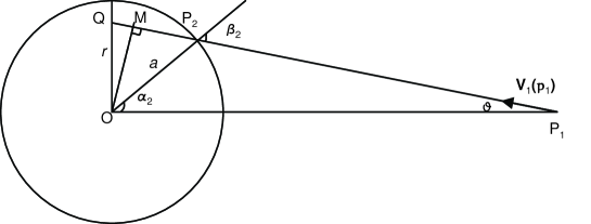
Figure 15: Particle obstacle Collision.

6.2 Algorithm description

In this section we describe the algorithm which we used in our program for Lorentz gas. We first define in the main of our program the initial conditions for the particles and the obstacles positions. In the second step, we compute with which obstacle, a particle will collide: we measure the angle between velocity of particle and the line between this particle and the center of obstacle, $\mathrm{OP}_{1}$ in Fig. 16, if this angle is less than or equal to the angle between this line, $\mathrm{OP}_{1}$, and the tangent line on the circle, i.e. $\mathrm{P_{1}N}$, in brief if $\vartheta\leq\varphi$ in Fig. 16, we have a collision. Now, we use the collision map equation (6.10) or (6.12) to obtain the collision angles, $\beta_{2}$, and $\alpha_{2}$ (see Fig. 15). In this step, we can also obtain the length of arrow of our induced collision map, i.e. $\mathrm{P_{1}P_{2}}$ (see Fig. 15), easily as:

$$\mathrm{P_{1}P_{2}}=\frac{\mathrm{OP_{1}}-a\cos\alpha_{2}}{\cos\vartheta}$$ (6.13)

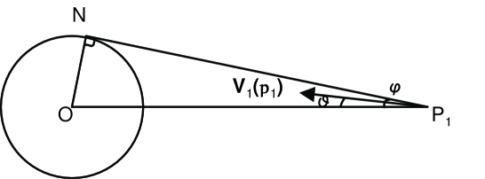
Figure 16: Particle obstacle Collision.

where $\alpha_{2}=\beta_{2}-\vartheta$. Then, we can calculate the time of flight of particle between two collisions, respectively, as $t=\mathrm{P}_{1}\mathrm{P}_{2}/v$. This provides the trajectory of a particles.
Let us turn the computation of space entropy. When a particle arrives at a wall of the big torus, before it does a collision with an obstacle (see on the Fig. 1) trajectories are pursued until it undergoes a collision on the torus. We have to compute the position of the obstacle that the particle will hit (see Fig. 17) and the angle $\alpha_{1}$ in the collision map, and to determine which type of collision, i.e. crossing or non-crossing case, will occur. We first find the angle of collision

$$\beta_{2}=\vartheta+\varphi=\arcsin[\frac{\mathrm{MO}_{2}}{a}\sin\vartheta],$$ (6.14)

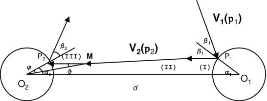
Figure 17: The motion of the particle take place on a tours.

then we arrive at $\alpha_{1}$ and $\alpha_{1}$ as

$$\left\{\begin{array}[]{ll}\alpha_{1}^{n}=\beta_{1}+\arcsin[\frac{a}{d}(\sin\beta_{2}-\sin\beta_{1})],&\alpha_{2}^{n}=\beta_{2}+(\beta_{1}-\alpha_{1})\\ \alpha_{1}^{c}=\beta_{1}-\arcsin[\frac{a}{d}(\sin\beta_{2}+\sin\beta_{1})],&\alpha_{2}^{c}=\beta_{2}-(\beta_{1}-\alpha_{1})\\ \end{array}\right.$$

(6.15)

where the superscript ”$c$” corresponds to crossing case and ”$n$” corresponds to non-crossing case see equations (6.10) and (6.12), respectively. In the above equations, the $d$ parameter is unknown, and will be recognized it in the end of this appendix. If we subtract the above equations we obtain

$$\alpha_{1}^{c}-\alpha_{1}^{n}=-\arcsin[\frac{a}{d}(\sin\beta_{2}+\sin\beta_{1})]-\ arcsin[\frac{a}{d}(\sin\beta_{2}-\sin\beta_{1})]$$ (6.16)

We can see the above equation yields $\alpha_{1}^{c}-\alpha_{1}^{n}\leq 0$. It means that in the same conditions the angle $\alpha_{1}$ in the non-crossing is greater than crossing case. Also, we can get the same conclusion for $\alpha_{2}$, i.e. $\alpha_{2}^{c}\leq\alpha_{2}^{n}$. Now, we initiate the algorithm in the non-crossing case and we find $\alpha_{1}^{c}$ and $\alpha_{2}^{n}$. If $\vartheta\leq\alpha_{2}$, thus, we had a correct supposition, otherwise, we must consider the crossing case, and we re-calculate these angles. In order to find in this case the parameter $d=|\mathrm{O}_{1}\mathrm{O}_{2}|$, we calculate it by approximation method. The equation that recognize $d$ is:

$$d=vdt\cos(\beta_{1}-\alpha_{1})+a(\cos\alpha_{1}+\cos\alpha_{2})$$ (6.17)

where $dt$ is the time of free flight of particle between two collisions, see Figs. (1 and 17 ). In the above equation we have two unknown variables, $\alpha_{1}$ and $\alpha_{2}$. We use the zeroth approximation as

$$d\approx vdt$$ (6.18)

where we used $a\ll vdt$. Now, we calculate the angles, $\alpha_{1}$ and $\alpha_{2}$, as mentioned in above of this appendix. Then, we re-calculate $d$ with the first approximation, and we can repeat this procedure. However, the convergence is very rapid.

References

- [1] R. Balescu, Equilibrium and Nonequilibrium Statistical Mechanics, John Wiley, New York, 1975.
- [2] G. Bennetin, L. Galgani, A. Giorogilli, J.M. Strelcyn, Lyapounov characteristic Exponents for smooth dynamical systems and for Hamiltonian systems; a method for all off them, Part 1 and 2, Meccanica 15 (1980) 9-30.
- [3] L.A. Bunimovich , Ya. G. Sinaï, Statistical properties of Lorentz gas with periodic configuration of scatterers. Comm. Math. Phys. 78 (1980/81), 479-497.
- [4] L. A. Bunimovich, Ya. G. Sinaï, N. I. Chernov, Markov partitions for two-dimensional hyperbolic billiards, Russian Math. Surveys 45 (1990), 105-152.
- [5] N.I. Chernov, L.S. Young, Decay of correlations for Lorentz gases and hard balls. Hard ball systems and the Lorentz gas, Encyclopaedia Math. Sci. No. 101, Springer, Berlin, 2000, pp 89-120.
- [6] M. Courbage, Intrinsic Irreversibility in Kolmogorov Dynamical Systems, Physica A 122 (1983), 459.
- [7] M. Courbage, B. Misra, On the equivalence between Bernoulli systems and stochastic Markov processes. Physica A 104 (1980), 359-377.
- [8] M. Courbage, G. Nicolis, Markov evolution and H-theorem under finite coarse-graining in conservative dynamical systems, Europhysics Letters 11 (1990), 1-6.
- [9] M. Courbage, I. Prigogine, Intrinsic randomness and intrinsic irreversibility in classical dynamical systems, Proc. Natl. Acad. Sci. USA 80 (1983), 2412-2416.
- [10] G. Gallavotti, D.S. Ornstein, Billiards and Bernoulli schemes , Commun. Math.Phys. 38, (1974), 83-101.
- [11] P.L. Garrido, S. Goldstein, J.L. Lebowitz, Boltzmann Entropy for dense fluids not in local equilibrium, Phys. Rev. Lett. 92, (2004), 050602.
- [12] P. Gaspard, H. Beijeren, When do tracer particles dominate the Lyapounov spectrum? J. Stat. Phys. 314 (2002), 671-704.
- [13] S. Goldstein, B.Misra and M. Courbage : On Intrinsic Randomness of Dynamical Systems. J.Stat.Phys. 25, 11-126, (1981).
- [14] S. Goldstein, O. Penrose, A nonequilibrium entropy for dynamical systems, J. Stat. Phys. 22 (1981), 325-343.
- [15] B.Misra, I.Prigogine, M.Courbage, From the Deterministic Dynamics to Probabilistic Descriptions, Physica A 98 (1979), 1-26.
- [16] YA.G. Sinaï, Dynamical systems with elastic reflections. Ergodic properties of dispersing billiards, Russ. Math. Survey 25 (1970) 137-189.
- [17] YA.G. Sinaï, Gibbs measures in ergodic theory, Russian Math. Surveys 27 (1972), no. 4, 21-69.
- [18] YA.G. Sinaï, Topics in Ergodic Theory Princeton University Press, Princeton 1994.
- [19] G.M. Zaslavsky, M.A. Edelman, Fractional kinetics: from pseudochaotic dyanamics to Maxwell’s Demon, Physica D 193 (2004), 128-147.