Controllable coupling of superconducting flux qubits

Abstract

We have realized controllable coupling between two three-junction flux qubits by inserting an additional coupler loop between them, containing three Josephson junctions. Two of these are shared with the qubit loops, providing strong qubit–coupler interaction. The third junction gives the coupler a nontrivial current–flux relation; its derivative (i.e., the susceptibility) determines the coupling strength $J$, which thus is tunable in situ via the coupler’s flux bias. In the qubit regime, $J$ was varied from $\sim$45 (antiferromagnetic) to $\sim$$-55$ mK (ferromagnetic); in particular, $J$ vanishes for an intermediate coupler bias. Measurements on a second sample illuminate the relation between two-qubit tunable coupling and three-qubit behavior.

The development of Josephson qubit devices has led to the realization of quantum gates Pashkin ; Yamamoto ; Chiorescu as well as two- Pashkin ; Berkley ; Izmalkov and four-qubit 4qb coupling. For the implementation of real quantum algorithms, several hurdles must still be cleared, such as increasing the number of qubits and their coherence times. Equally important, however, is coupling tunability. If the coupling strength can be continuously tuned between two values with opposite signs, it can be naturally switched off—a great advantage when applying two-qubit gates untun . Moreover, in adiabatic quantum computing, continuously tuning the Hamiltonian is crucial, and both ferromagnetic (FM) and antiferromagnetic (AF) couplings are necessary AQC_SC . In a promising group of proposals, coupling capacitances and inductances are replaced with effective (“quantum”) capacitances AB and inductances Clarke_coupler ; Alec_Berkley , respectively, which are (sign-)tunable via their bias dependence.

We report the realization of sign-tunable coupling Harris between three-Josephson-junction (3JJ) flux qubits Mooij . These have a low charge-noise sensitivity, common to all flux qubits. Their small area also protects them reasonably well against magnetic noise, but limits the strength of their AF coupling via magnetic Izmalkov and/or kinetic majer inductance. This can be overcome by using a Josephson mutual inductance Delft_ladder , which can also be “twisted” for FM coupling or (in theory) current-biased for limited tunability Coupling2005 . Our design Alec_note combines the above ideas, mediating a tunable galvanic coupling through a “quantum Josephson mutual inductance”. The coupler is connected to qubits $a$ and $b$ via shared junctions 7 and 9, see Fig. 1. By changing the coupler’s flux bias $\Phi_{\mathrm{c}}^{\mathrm{x}}=f_{\mathrm{c}}\Phi_{0}$ ($\Phi_{0}$ is the flux quantum), the phase difference across junction 8 and therefore the interaction strength $J$ can be tuned. The fluxes through the coupler and qubits are controlled by bias-line currents $I_{\mathrm{b1,2,3}}$ and the dc component $I_{\mathrm{bT}}$ of the coil current compensation .

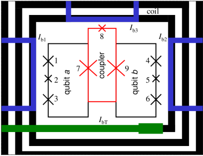
Figure 1: Circuit design of sample 1. Junctions 123 (456) form qubit a (b). The large qubit junctions have areas $S_{1,3,4,6}=150\times 700$ nm², while $\alpha_{a,b}\equiv S_{2,5}/S_{1}=0.65$. Junctions 789 form the coupler (red), with areas $S_{7,9}=150\times 2000$ nm² and $S_{8}=150\times 400$ nm². The ratio between the coupler and qubit loop areas is $1:2$. The tank circuit has inductance $L=90$ nH and capacitance $C=470$ pF, yielding a resonance at $\omega_{\mathrm{T}}/2\pi=20.76$ MHz with quality $Q=300$. The mutual inductances, deduced from the flux periodicity, are $M_{a,\mathrm{T}}=M_{b,\mathrm{T}}=98$, $M_{\mathrm{c,T}}=51$, $M_{a,\mathrm{b1}}=0.85$, $M_{b,\mathrm{b1}}=0.17$, $M_{\mathrm{c,b1}}=0.19$, $M_{a,\mathrm{b2}}=0.23$, $M_{b,\mathrm{b2}}=1.2$, $M_{\mathrm{c,b2}}=0.25$, $M_{a,\mathrm{b3}}=0.42$, $M_{b,\mathrm{b3}}=0.39$, and $M_{\mathrm{c,b3}}=0.56$ (all in pH).

The system can be described by the effective pseudospin Hamiltonian Mooij ; Izmalkov ; Chiorescu

$$H=-\sum_{i=a,b}[\epsilon_{i}\sigma_{z}^{(i)}+\Delta_{i}\sigma_{x}^{(i)}]+J(\phi_{\mathrm{c}})\sigma_{z}^{(a)}\sigma_{z}^{(b)}\;,$$ (1)

where $\epsilon_{i}$ is the bias on qubit $i$, $\Delta_{i}$ is the corresponding tunnelling matrix element, $\sigma_{z}^{(i)}$, $\sigma_{x}^{(i)}$ are Pauli matrices in the flux basis, and $\phi_{\mathrm{c}}\equiv 2\pi f_{\mathrm{c}}$.

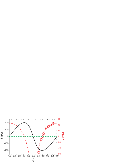
Figure 2: Black: the current–flux relation $I(f_{\mathrm{c}})$ of a coupler with $\alpha_{\mathrm{c}}=S_{8}/S_{9}=0.2$ and $I_{\mathrm{c}}=1~{}\mu$A. Red-dashed line: the coupling energy $J(f_{\mathrm{c}})$ obtained from Eq. (3) using this $I(f_{\mathrm{c}})$ and the loop currents $I_{\mathrm{p}a,b}$ found independently from the qubit response. Circles: experimental $J(f_{\mathrm{c}})$ obtained from Fig. 3.

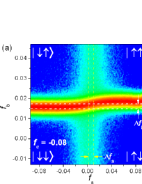
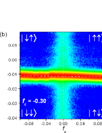
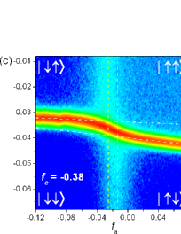
Figure 3: $-\tan\theta(f_{a},f_{b})$ for sample 1 at coupler bias $f_{\mathrm{c}}=-0.08$, $-0.30$, and $-0.38$, with a manifest change in coupling sign. A theory fit as in Fig. 4 yields couplings $J=45$, $0$, and $-55$ mK. The excess response in the $\lvert{\uparrow\uparrow}\rangle$ quadrant for $f_{\mathrm{c}}=-0.38$ is due to the coupler.

To calculate $J$ for a coupler with symmetric Josephson energies $E_{7,9}=E$, $E_{8}=\alpha_{\mathrm{c}}E$, consider the potential

$$\begin{split}U_{\mathrm{J}}(\bm{\phi})&=-E[\cos\phi_{7}+\alpha_{\mathrm{c}}\cos(\phi_{\mathrm{c}}{-}\phi_{7}{-}\phi_{9})+\cos\phi_{9}]\\ &\quad\,+U_{a}(\phi_{a}{+}\phi_{7})+U_{b}(\phi_{b}{+}\phi_{9})\;,\end{split}$$ (2)

where we implemented flux quantization for small-inductance loops, with $\phi_{a,b}$ being the qubit flux biases in phase units, and where the qubit energies $U_{a,b}$ are already minimized over their internal degrees of freedom $\phi_{\text{1--6}}$. However, each qubit has two minimum states, with opposite values of the persistent currents $-(2e/\hbar)U_{a,b}^{\prime}=\pm I_{\mathrm{p}a,b}$. We minimize $U_{\mathrm{J}}(\bm{\phi})$ with respect to $\phi_{7,9}$, and expand in $E^{-1}$. This implements the classical limit of the general condition that the coupler should stay in its ground state, following the qubits adiabatically AB . To leading order, the phases obey $\phi_{7}=\phi_{9}=\bar{\phi}$, with $\sin\bar{\phi}=\alpha_{\mathrm{c}}\sin(\phi_{\mathrm{c}}{-}2\bar{\phi})$. Proceeding to $\mathcal{O}(E^{-1})$ and retaining terms $\propto I_{\mathrm{p}a}I_{\mathrm{p}b}$, one finds J-note

$$J(\phi_{\mathrm{c}})=\frac{\hbar}{2e}\frac{I^{\prime}(\phi_{\mathrm{c}})}{I_{\mathrm{c}}^{2}-I(\phi_{\mathrm{c}})^{2}}\,I_{\mathrm{p}a}I_{\mathrm{p}b}\;,$$ (3)

in terms of the coupler current $I(\phi_{\mathrm{c}})=I_{\mathrm{c}}\sin\bar{\phi}$ with $I_{\mathrm{c}}=(2e/\hbar)E$, so that

$$I^{\prime}(\phi_{\mathrm{c}})=I_{\mathrm{c}}\frac{\cos(\bar{\phi})\alpha_{\mathrm{c}}\cos(\phi_{\mathrm{c}}{-}2\bar{\phi})}{\cos(\bar{\phi})+2\alpha_{\mathrm{c}}\cos(\phi_{\mathrm{c}}{-}2\bar{\phi})}\;.$$ (4)

The numerator in Eq. (3) also occurs for magnetic coupling Alec_Berkley ; the denominator reflects, for finite coupler-loop currents, the nonlinearity of the Josephson elements 7 and 9. Figure 2 shows $I$ and $J$ for $\alpha_{\mathrm{c}}=0.2$. If $\alpha_{\mathrm{c}}\ll\nobreak 1$, $I(\phi_{\mathrm{c}})\approx\alpha_{\mathrm{c}}I_{\mathrm{c}}\sin\phi_{\mathrm{c}}$, i.e., $J(\phi_{\mathrm{c}})\approx\linebreak[1]I_{\mathrm{p}a}I_{\mathrm{p}b}\*\hbar^{2}\alpha_{\mathrm{c}}\cos\phi_{\mathrm{c}}/4e^{2}E$ Alec_note . Hence, $J(\phi_{\mathrm{c}})>0$ ($<\nobreak 0$) near $\phi_{\mathrm{c}}=0$ ($\pi$) extreme , corresponding to AF (FM) coupling. However, Fig. 2 already is strongly non-sinusoidal, with a larger maximum for FM than for AF coupling (cf. Ref. Alec_Berkley ).

The qubit–coupler circuit was fabricated out of aluminum, and the pancake coil out of niobium Izmalkov ; 4qb . Besides providing an overall dc field bias, the coil is part of an $LC$ tank circuit driven at resonance, well below the characteristic qubit frequencies. In the Impedance Measurement Technique Grajcar , one records the tank’s current–voltage phase angle $\theta$, which is very sensitive to its effective inductance: $\tan\theta=-(Q/L)\chi^{\prime}$, where $Q$ and $L$ are the tank’s quality factor and “bare” inductance, respectively, and $\chi^{\prime}$ is the contribution to the tank inductance due to the qubits’ reactive susceptibility. In the coherent regime, $\chi^{\prime}$ has peaks at level anticrossings greenberg , where a small bias $\epsilon_{i}\sim\Delta_{i}$ will flip the flux state of qubit $i$. Thus, these peaks demarcate the qubits’ stability diagram, from which $J$ can be read off Coupling2005 , while their widths are $\propto\Delta_{i}$.

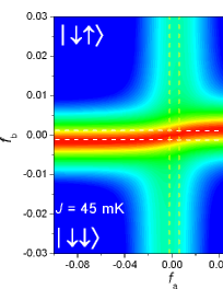
Figure 4: Theoretical fit for Fig. 3a. The extracted parameters are $T_{\mathrm{eff}}=70$ mK, $\Delta_{a}=300$ mK, $I_{\mathrm{p}a}=75$ nA, $\Delta_{b}=55$ mK, $I_{\mathrm{p}b}=180$ nA, and $J(-0.08)\approx 45$ mK.

All measurements were performed in a dilution refrigerator with a base temperature of 10 mK. Results for sample 1 are presented in Fig. 3 around the qubits’ co-degeneracy point [$\epsilon_{a}=\epsilon_{b}=0$ in (1)], for fixed compensation coupler fluxes $f_{\mathbf{c}}=-0.08$, $-0.30$, and $-0.38$. In Fig. 3a, the FM ordered $\lvert{\uparrow\uparrow}\rangle$ and $\lvert{\downarrow\downarrow}\rangle$ states are pushed away from this point, where the $\lvert{\uparrow\downarrow}\rangle$ and $\lvert{\downarrow\uparrow}\rangle$ states dominate—a clear signature of AF coupling. In Fig. 3b, the $a$- (vertical) and $b$-traces (horizontal) are independent, demonstrating zero coupling. Finally, Fig. 3c is opposite to Fig. 3a, corresponding to FM coupling.

Quantitatively, the state of the system (1) at temperature $T_{\mathrm{eff}}$ is readily calculated; the effect on the tank flux follows from the mutual inductances as in Fig. 1, and taking the $I_{\mathrm{bT}}$-derivative yields $\chi^{\prime}$. Fitting this equilibrium response to the data, all parameters in Eq. (1) as well as $T_{\mathrm{eff}}$ can be extracted Izmalkov ; 4qb ; Coupling2005 ; Grajcar . From the shape of the single-qubit traces, one finds $\Delta_{a,b}$ and $I_{\mathrm{p}a,b}$; the shifts $\Delta f_{a,b}$ in these traces when they cross the co-degeneracy point yield $J=\frac{1}{2}\Delta f_{a,b}\Phi_{0}I_{\mathrm{p}a,b}$. That is, here we foremost measure $H$, not the qubit state $\lvert{\Psi}\rangle$. As an example, Fig. 4 shows a fit to Fig. 3a, yielding $T_{\mathrm{eff}}\approx 70$ mK, $\Delta_{a}=300$ mK, $I_{\mathrm{p}a}=75$ nA, $\Delta_{b}=55$ mK, $I_{\mathrm{p}b}=180$ nA, and $J\approx 45$ mK. The agreement between theory and experiment confirms that the system is in the qubit regime.

The $J(f_{\mathrm{c}})$ thus measured (Fig. 2) agrees with Eq. (3) for the design value $\alpha_{\mathrm{c}}=0.2$, and $I_{\mathrm{c}}=1~{}\mu$A for the coupler. Note that $J(f_{\mathrm{c}}{=}{-}0.30)\linebreak[1]=0$ already implies $\alpha_{\mathrm{c}}\approx 0.2$ by Eqs. (3) and (4); $I_{\mathrm{c}}=1~{}\mu$A is consistent with $I_{\mathrm{c}}\approx\linebreak[1](S_{9}/S_{6})\*I_{\mathrm{p}b}/\sqrt{1-1/4\alpha^{2}}\approx 0.8~{}\mu$A, expected from $I_{\mathrm{p}b}$ ($S_{6}$, $S_{9}$ are the respective junction areas).

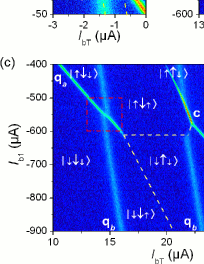
Figure 5: $-\tan\theta(I_{\mathrm{bT}},I_{\mathrm{b1}})$ for sample 2. (a) $I_{\mathrm{b2}}=0$. At co-degeneracy, the coupler flux is $f_{\mathrm{c}}=0.237$, and the induced coupling $J\approx 85$ mK. (b) and (c) $I_{\mathrm{b2}}=450$ $\mu$A. (b) Close-up of the co-degeneracy point [dashed box in (c)], where $f_{\mathrm{c}}=0.347$ and $J\approx 44$ mK. (c) Overview and stability diagram. At bias points outside the boxed area, the coupler itself can become bistable, and contribute its own anticrossing to the impedance response. The arrow sizes denote the relative magnitudes of the loop currents in qubit $a$, coupler, and qubit $b$ respectively.

A sample 2 was fabricated with $\alpha_{\mathrm{c}}=0.5$, i.e., a larger junction 8 and hence potentially a stronger coupling. Figure 5 presents results for $\tan\theta(I_{\mathrm{bT}},I_{\mathrm{b1}})$. In Fig. 5a, $I_{\mathrm{b2}}=0$. The qubits are at co-degeneracy for $f_{\mathrm{c}}=0.237$. A theoretical fit as for sample 1 gives $I_{\mathrm{p}a}=130$ nA, $I_{\mathrm{p}b}=70$ nA, $\Delta_{a}\approx\Delta_{b}\approx 70$ mK, and $J\approx 85$ mK. In Fig. 5b, a bias current $I_{\mathrm{b2}}=450~{}\mu$A is applied. As a result, the co-degeneracy point is shifted to $f_{\mathrm{c}}=0.347$. Compared with Fig. 5a, the coupling strength is reduced to $J=85\times(0.30/0.58)\approx 44$ mK.

For $\alpha_{\mathrm{c}}=0.5$, the negative-slope portion of $I(f_{\mathrm{c}})$ (cf. Fig. 2) is very narrow, so that FM coupling should only occur for $|f_{\mathrm{c}}{-}{\textstyle\frac{1}{2}}|\ll 1$. Hence, in sample 2 only the (AF) coupling strength could be varied, not its sign. In fact, the coupler is on the very boundary of the hysteretic regime Mooij . Hence, for $f_{\mathrm{c}}\approx{\textstyle\frac{1}{2}}$, the energy gap above the ground state will be very small and the adiabaticity condition mentioned above Eq. (3) breaks down, regardless of the exact value of $\alpha_{\mathrm{c}}-{\textstyle\frac{1}{2}}$. Indeed, in this case we rather observe three-qubit behavior, with the coupler’s own anticrossing characterized by $\Delta_{\mathrm{c}}=90$ mK and $I_{\mathrm{pc}}=300$ nA (Fig. 5c). This is fully consistent with our interpretation above, since the operating regimes are different.

In conclusion, we have for the first time demonstrated sign-tunable Josephson coupling between two three-junction flux qubits, in the quantum regime. At $T_{\mathrm{eff}}\approx 70$ mK, the coupling strength $J$ was changed from +45 (antiferromagnetic) to $-55$ mK (ferromagnetic). At an intermediate coupler bias, $J$ vanishes, thereby realizing the elusive superconducting switch. These results represent considerable progress towards solid-state quantum computing in general. The present low-frequency mode of operation is particularly attractive for adiabatic quantum computing: control of $J>0$ is necessary to operate the computer, and sufficiently strong ferromagnetic coupling ($J<0$) allows one to create dummy qubits, as used in the scalable architecture of Ref. AQC_SC . While our measurements are essentially equilibrium, the design of Fig. 1 is also relevant in the ac domain, where the coupling can be controlled by a resonant rf signal ac-tune .

AMvdB thanks M.H.S. Amin, J.M. Martinis, and A.Yu. Smirnov for discussions, and the ITP (Chinese Univ. of Hong Kong) for its hospitality. SvdP, AI, and EI were supported by the EU through the RSFQubit and EuroSQIP projects, MG by Grants VEGA 1/2011/05 and APVT-51-016604 and the Alexander von Humboldt Foundation, and AZ by the NSERC Discovery Grants Program.

Note added.—Recently, we learned of the work of Hime et al. Hime implementing the controllable-coupling proposal described in Ref.Clarke_coupler .

References

- (1) Yu.A. Pashkin et al., Nature 421, 823 (2003).
- (2) T. Yamamoto et al., Nature 425, 941 (2003).
- (3) I. Chiorescu et al., Nature 431, 159 (2004).
- (4) A.J. Berkley et al., Science 300, 1548 (2003).
- (5) A. Izmalkov et al., Phys. Rev. Lett. 93, 037003 (2004).
- (6) M. Grajcar et al., Phys. Rev. Lett. 96, 047006 (2006).
- (7) Alternatives to coupling switchability require at least a large hardware overhead: e.g., X. Zhou et al., Phys. Rev. Lett. 89, 197903 (2002).
- (8) W.M. Kaminsky, S. Lloyd, and T.P. Orlando, quant-ph/0403090; M. Grajcar, A. Izmalkov, and E. Il’ichev, Phys. Rev. B 71, 144501 (2005).
- (9) D.V. Averin and C. Bruder, Phys. Rev. Lett. 91, 057003 (2003).
- (10) B.L.T. Plourde et al., Phys. Rev. B 70, 140501(R) (2004).
- (11) A. Maassen van den Brink, A.J. Berkley, and M. Yalowsky, New J. Phys. 7, 230 (2005).
- (12) For the experimental realization of the proposal of Ref. Alec_Berkley ,see R. Harris et al., Phys. Rev. Lett. 98, 177001 (2007) and V. Zakosarenko et al., Appl. Phys. Lett. 90, 022501 (2007). For a different implementation of tunable coupling, see M.G. Castellano et al., Appl. Phys. Lett. 86, 152504 (2005).
- (13) J.E. Mooij et al., Science 285, 1036 (1999); T.P. Orlando et al., Phys. Rev. B 60, 15398 (1999).
- (14) J.B. Majer et al., Phys. Rev. Lett. 94, 090501 (2005).
- (15) L.S. Levitov et al., cond-mat/0108266; J.R. Butcher, graduation thesis (Delft University of Technology, 2002); for an application to charge–phase qubits, see J.Q. You, J.S. Tsai, and F. Nori, Phys. Rev. B 68, 024510 (2003); for a related design featuring some tunability, see M.D. Kim and J. Hong, Phys. Rev. B 70, 184525 (2004).
- (16) M. Grajcar et al., Phys. Rev. B 72, 020503(R) (2005).
- (17) A. Maassen van den Brink, cond-mat/0605398.
- (18) For sample 1, is used to set the overall magnetic field, while in combination facilitate independent tuning of the biases in qubits and coupler using a flux-compensation procedure. Sample 2 does not have a wire and is measured without flux compensation.
- (19) Since corrections are , with , Eq. (3) should be a reasonable approximation.
- (20) The values are of interest not only because they maximize the coupling strength, but also because the stationary points of have minimum sensitivity to coupler-bias noise. Compare A.O. Niskanen, Y. Nakamura, and J.-S. Tsai, Phys. Rev. B 73, 094506 (2006).
- (21) E. Il’ichev et al., Fiz. Nizk. Temp. 30, 823 (2004); Low Temp. Phys. 30, 620 (2004).
- (22) Ya.S. Greenberg et al., Phys. Rev. B 66, 214525 (2002).
- (23) M. Grajcar et al., Phys. Rev. B 74, 172505 (2006).
- (24) T. Hime et al., Science 314, 1427 (2006).