Spin currents in the Rashba model in the presence of non-uniform fields

Abstract

Spin currents in a two dimensional electron gas with Rashba-type spin orbit coupling are derived from a spin connection.  Using a functional integral method, we recover the result derived by Sinova et al.$\left[\mathrm{Phys.Rev.Lett.92,126603(2004)}\right]$ for a uniform electric field and in the absence of impurities.  We extend this result to inhomogeneous electric and magnetic fields.  We find that non-uniform magnetic fields can give rise to spin currents that are independent of the Rashba coupling and hence are less susceptible to impurities than in the case of uniform electric fields.

Spin-orbit coupling (SOC) of the conduction electrons in two dimensional systems is of special importance in magnetic and semiconductor materials.  It was recently realized that SOC can be used to manipulate the spin of the conduction electrons in semiconductors.  An interesting outcome of this coupling is that an equilibrium spin current in semiconductors becomes possible due to SOC in the presence of an in-plane electric field das .  This topic is currently of considerable interest since the question on the size of this current is still open.  One of the reasons for this lack of agreement is that there is no rigorous definition for these currents because they are not conserved in a medium with a spin orbit coupling rashba1 ; rashba2 .

In this note, we point out a well defined procedure for calculating spin currents through first defining a spin connection FS similar to the procedure of defining charge currents with respect to a $U(1)$ connection.  We discuss the simple two dimensional system of an electron gas with spin-orbit Rashba-type coupling sinova .  The Rashba coupling describes well the dynamics of conduction electrons in semiconductors, e.g., GaAs, which are potentially important materials for spintronics. Similarly, the Rashba model is of interest to conduction electrons in magnetic thin films and the damping problem of the magnetization in these materials.  We will treat two cases; first a 2-dimensional electron gas with SOC in the presence of an electric field directed in-plane, and second with an inhomogeneous magnetic field and electric field.  The first case has already been treated by Sinova et al. sinova and others, while the non-uniform magnetic field case is new.  It also has a universal behavior and hence less susceptible to be destroyed by impurity scaatering.

The recent result by Sinova et al. sinova that spin currents are possible in systems described by Rashba coupling attracted considerable attention inoue ; raimondi ; loss ; chalaev ; bernevig ; chao ; chao2 ; niu ; sun because of its universal features .  The value of $|e|/8\pi$ for the spin Hall conductivity is independent of the strength of the SOC.  Since spin is not conserved in this system, much debate has been centered around the question of what is the correct way to define the corresponding spin current.  In the following, we argue that the best way to approach the question of what is the appropriate equation for the spin current, is by first identifying the associated $SU(2)$ spin connection to the current, if such one exists.  Then, we calculate the effective action of the 2DEG from which a definition of the spin current follows unambiguously by differentiation with respect to the $SU(2)$ connection.  This procedure is well known in Gauge theory schwinger ; IZ .

The Rashba Hamiltonian for a two-dimensional electron gas (2DEG) is given by bychkov

$$H_{0}=\frac{1}{2m}\left(p_{x}^{2}+p_{y}^{2}\right)+\lambda\left(p_{y}\sigma_{x}-p_{x}\sigma_{y}\right),$$ (1)

where $\lambda$ is a coupling constant, $m$ is the effective mass of the electron in the lattice, $\mathbf{\sigma}$ is a Pauli matrix vector, and we use units such that $\hbar=c=1$.  The spin vector of the electron is $\mathbf{S}=\frac{1}{2}\mathbf{\sigma}$ and its magnetic moment is $\mu=-\frac{e}{2m}\;(e<0)$.  The action of this system is clearly $U(1)$ invariant and this gives a continuity equation for the charge.  Therefore, we naturally seek a continuity equation for the spin by first finding under what conditions this system has a $SU(2)$ symmetry which is generated by a spin charge.  This question was first asked by Frohlich and Studer FS for a general non-relativistic particle interacting in an electromagnetic field.  They were able to show that such systems exhibit a $U(1)\times SU(2)$ symmetry and hence a corresponding charge current and spin current follow directly from this gauge symmetry.  Following this procedure, we can ask similar questions for the Rashba system and this will allow us to identify a spin connection and the corresponding covariant derivatives.  It is well known from Gauge theories, that currents with sources will not be continuous but only covariantly continuous.

In mathematical terms, we want to see if it is possible to express the equation of motion for the electrons in the following form

$$i\frac{\partial\psi}{\partial t}=-\frac{1}{2m}\left(\mathcal{D}_{k}\mathcal{D}^{k}\right)\psi+eA_{0}\psi+g\mu\mathbf{V}_{0}\cdot\mathbf{S}\psi,$$ (2)

where $g=2$ for an electron in vacuum and the spatial covariant derivative is $\mathcal{D}_{k}=\nabla_{k}+ieA_{k}+i(g-1)\mu\mathbf{V}_{k}\cdot\mathbf{S}$.   $\mathbf{A}$ is the usual $U(1)$ field and $\mathbf{V}$ is the sought after tensor field associated with the $SU(2)$ gauge or spin charge.  This way of writing the covariant derivative clearly displays that charge currents are associated with the charge $e$ of the electrons while spin currents are associated with the magnetic moment $\mu$.  Therefore a spin current $\textsl{j}_{k}=\textsl{j}_{k}^{\alpha}S_{\alpha}$ (summation implied) may exist in a system with zero charge but nonzero magnetic moments and will satisfy a ’continuity’ equation, $\mathcal{D}_{k}\textsl{j}^{k}=0;\;k=0,1,2,3$.  This is the result we show in this paper within a linear response approach.  Hence in the following we neglect second order terms in the potential. This is equivalent to taking $e$ and $\mu$ as small parameters.

The case of a constant electric field in the $xy$-plane and in the $x$-direction has been well studied in the recent literature.  Therefore in the following, we focus on the homogeneous time-dependent case.  The requirement of gauge invariance under $U(1)\times SU(2)$ for the Rashba action requires that $\mathbf{V}_{0}=-\mathbf{B}$ and $V_{k\alpha}=-\in_{k\alpha\beta}E_{\beta}$ for $k=x,y$ and $\alpha,\beta=1,2,3$ (We use Greek or numerical indexes to denote spin components).  The Rashba coupling $\lambda$ can be thought of as due to a fictitious electric field perpendicular to the $xy-$plane of the 2DEG, $\lambda=\frac{e}{4m^{2}}E_{z}$.  The Rashba interaction is therefore replaced by $H_{SOC}=\lambda\left(p_{y}\sigma_{1}-p_{x}\sigma_{2}\right)-\frac{e}{4m^{2}}p_{x}\sigma_{3}E_{x}$.  For an electric field $\mathbf{E}=-\frac{1}{c}\partial\mathbf{A}/\partial t$ in the $x$-direction, the interaction term becomes to first order in the potential

$$H_{int}=\frac{e}{m}A_{x}(\mathbf{r},t)(p_{x}-{\lambda m}\sigma_{2}).$$ (3)

In the following we take $E_{z}>>E_{x}$ and hence the additional spin orbit coupling due to the E field in the $x$-direction can be neglected.  The $E_{z}$ field will therefore be treated as a background field in the following.

The generating functional of the theory is given by

$$Z\left[\mathbf{A},\mathbf{V}\right]=$$ (4)

$$\int D\psi^{\dagger}D\psi\exp\left\{i\int dtd^{2}x\;\left[\psi^{\dagger}\left(t,\mathbf{r}\right)\left(G^{-1}\right)\psi\left(t,\mathbf{r}\right)\right.\right.$$

$$\left.\left.+\psi^{\dagger}\left(t,\mathbf{r}\right)\psi\left(t,\mathbf{r}\right)K\psi^{\dagger}\left(t,\mathbf{r}\right)\psi\left(t,\mathbf{r}\right)\right]\right\},$$

where we have included scattering due to impurities by a potential $U$ , with $\left\langle U(r)U(r^{\prime})\right\rangle=K\delta\left(r-r^{\prime}\right)$ where $K=1/(m\tau)$ and $\tau$ is the scattering. The propagator of the theory is given by

$$G^{-1} = i\partial_{t}-\frac{1}{2m}\pi^{2}-\frac{(g-1)\mu}{2m}\left[\mathbf{S}\cdot\mathbf{V}_{k},\pi_{k}\right]_{+}-g\mu\mathbf{S}\cdot\mathbf{V}_{0},$$ (5)

where $\left[,\right]_{+}$ is the anti-commutator operation, $\pi_{l}=p_{l}+eA_{l}$ and $g=2$ for an electron in vacuum.  In the absence of impurity scattering, the path integral can be easily integrated to get the effective action of the theory

$$\Gamma^{eff}\left[\mathbf{A},\mathbf{V}\right]=-i\;{\rm Tr}\;\log i\;G^{-1},$$ (6)

where the trace is over space and spin indexes.    The case of nonzero-potential in the ladder approximation has been treated in Ref. [mish, ] using a Boltzmann-type approach.  To simplify our discussion, we set the impurity potential to zero in the rest of this paper since our aim here is mainly to demonstrate the spin connection approach.  We first briefly treat the case of a constant electric field and then discuss the inhomogeneous magnetic and electric fields.  The spin current at $\mathbf{x}=(t,\mathbf{r})$ in the $y$-direction and polarized in the $z$-direction is therefore given by IZ

$$\frac{1}{\mu}\frac{\delta\Gamma^{eff}}{\delta V_{y3}(\mathbf{x})}=-\textsl{j}_{y3}(\mathbf{x}).$$ (7)

This definition reduces to the usual definition of spin currents FS .  In the linear response regime, we need only to calculate $G\left(\mathbf{\ x},\mathbf{x}^{\prime}\right)=G_{0}\left(\mathbf{\ x},\mathbf{x}^{\prime}\right)+\Sigma\left(\mathbf{\ x},\mathbf{x}^{\prime}\right)$ to first order in $E_{x}$ where $G_{0}$ is the $2\times 2$ Green’s function in the absence of the $E_{x}$ field, and its diagonal terms are given by $G_{0}^{11}\left(\omega\mathbf{\ },\mathbf{k}\right)=G_{0}^{22}\left(\omega\mathbf{\ },\mathbf{k}\right)=\left(\omega-\frac{k^{2}}{2m}\right)/\left[\left(\omega-\frac{k^{2}}{2m}\pm i\epsilon\right)^{2}-\lambda^{2}k^{2}\right]$, while the off-diagonal ones are $G_{0}^{12}\left(\omega\mathbf{\ },\mathbf{k}\right)=G_{0}^{21\ast}\left(\omega\mathbf{\ },\mathbf{k}\right)=\left(-i\lambda\left(k_{x}-ik_{y}\right)\right)/\left[\left(\omega-\frac{k^{2}}{2m}\pm i\epsilon\right)^{2}-\lambda^{2}k^{2}\right]$.  The poles of the Green function $G$ give the energy of the spin up and spin down states of the system.  Since $G_{11}^{0}=G_{22}^{0}$, only the $\Sigma$-term contributes to the $(y3)$-component of the spin current which becomes

$$\textsl{j}_{y3}=-\frac{1}{2im}{\rm Tr}\left\{\sigma_{3}p_{y}G^{0}\left(p_{x}+\lambda\;m\;\sigma_{2}\right)\;K\;G^{0}\right\}$$ (8)

with $K=\frac{e}{2m}\left\{A_{x},p_{x}\right\}$.  To find the spin current, we go to Euclidean time $t_{E}=it$.  The Fourier transform of the spin current for uniform fields is

$$\textsl{j}_{y3}\left(\omega\right) = =\frac{e\lambda}{4\pi m}E(\omega)\int_{k_{-}}^{k_{+}}dk\frac{k^{2}}{4\lambda^{2}k^{2}+\omega^{2}},$$ (9)

where $k_{\pm}=k_{F}\pm m\lambda$ are the momenta of the two bands and $k_{F}$ is the Fermi momentum, Fig. 1.  Only states below the Fermi energy are occupied. The static limit is therefore given by

$$\frac{\textsl{j}_{y3}(0)}{E(0)}=(g-1)\frac{\left|e\right|}{8\pi\hbar},$$ (10)

where we have restored physical units.  This result is equal to the one derived by Sinova et al. sinova and others loss in the absence of any scattering.  In the presence of impurities, it was shown in Refs. [mish, ] and [chalaev, ] that no matter how small the scattering by the impurities it cancels the spin Hall current.  Hence it is natural to ask what happens if the electric or magnetic fields are not uniform as is usually the case in real devices.

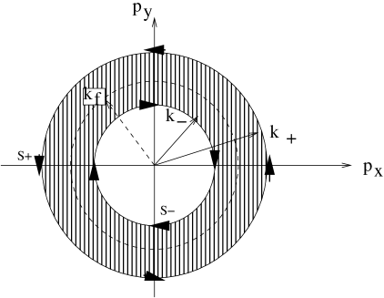
Figure 1: Fermi surfaces of the two bands in the Rashba model, $k_{\pm}=k_{F}\pm m\lambda$.  The tangential arrows are the spin projections on the $k_{x}k_{y}$ plane.  The point $k=0$ is a singular point.

In order to shed some light on this question, we extend our treatment to non-uniform vector potential fields.  We only calculate spin currents in the $(y3)$ direction.  We allow for both an electric field and a magnetic field to be applied to the Rashba electron gas.  The vector potential $\mathbf{A}=\left(A_{x},A_{y},A_{z}\right)$ is allowed to depend on both plane coordinates, $x$ and $y$.  To calculate the spin current in the static limit, we use a gradient expansion to the effective action.  In $QED_{2+1}$ such an expansion in momentum space gives rise to the well-known Chern-Simons term.das2  In our non-relativistic case, a real-space expansion is much easier to carry out than in momentum space and this is what we do here.  In the following, we keep only terms up to second order derivatives in the vector potential. The calculation is carried out in the transverse gauge, $\mathbf{k}\cdot\mathbf{A}(k)=0$.   The spin current in the $(y3)$ direction has two contributions, one coming from the kinetic term and the other from the Zeeman term.  The kinetic term gives a contribution of the form

$$J_{\mathbf{A}}\left(\mathbf{r},\omega\right) = \left(g-1\right)\left(a_{1}\left(\omega\right)A_{x}\left(\mathbf{r},\omega\right)+b_{1}\left(\omega\right)\frac{\partial^{2}A_{x}\left(\mathbf{r},\omega\right)}{\partial x^{2}}\right.$$ (11)

$$\left.+b_{2}\left(\omega\right)\frac{\partial^{2}A_{x}\left(\mathbf{r},\omega\right)}{\partial y^{2}}+c_{1}\left(\omega\right)\frac{\partial^{2}A_{y}\left(\mathbf{r},\omega\right)}{\partial y\partial x}\right).$$

where the frequency dependent coefficients are given by

$$a_{1}\left(\omega\right)=\frac{ie\lambda}{2m}\int\frac{d^{2}k_{1}}{(2\pi)^{2}}\frac{d\omega_{1}}{2\pi}tr\left\{\sigma^{3}G^{0}\left(\mathbf{k}_{1},\omega_{1}\right)\sigma^{2}G^{0}\left(\mathbf{k}_{1},\omega_{1}-\omega\right)\right\}k_{1}^{y},$$ (12)

$$b_{1}\left(\omega\right) = \frac{ie}{4m}\int\frac{d^{2}k_{1}}{(2\pi)^{2}}\frac{d\omega_{1}}{2\pi}tr\left\{\sigma^{3}G^{0}\left(\mathbf{k}_{1},\omega_{1}\right)\partial_{k_{x}}^{2}G^{0}\left(\mathbf{k}_{1},\omega_{1}-\omega\right)\right\}k_{1}^{x}k_{1}^{y}$$

$$-\frac{ie\lambda}{4m}\int\frac{d^{2}k_{1}}{(2\pi)^{2}}\frac{d\omega_{1}}{2\pi}tr\left\{\sigma^{3}G^{0}\left(\mathbf{k}_{1},\omega_{1}\right)\sigma^{2}\partial_{k_{x}}^{2}G^{0}\left(\mathbf{k}_{1},\omega_{1}-\omega\right)\right\}k_{1}^{y},$$

$$b_{2}\left(\omega\right) = \frac{ie}{4m}\int\frac{d^{2}k_{1}}{(2\pi)^{2}}\frac{d\omega_{1}}{2\pi}tr\left\{\sigma^{3}G^{0}\left(\mathbf{k}_{1},\omega_{1}\right)\partial_{k_{y}}^{2}G^{0}\left(\mathbf{k}_{1},\omega_{1}-\omega\right)\right\}k_{1}^{x}k_{1}^{y}$$

$$-\frac{ie\lambda}{4m}\int\frac{d^{2}k_{1}}{(2\pi)^{2}}\frac{d\omega_{1}}{2\pi}tr\left\{\sigma^{3}G^{0}\left(\mathbf{k}_{1},\omega_{1}\right)\sigma^{2}\partial_{k_{y}}^{2}G^{0}\left(\mathbf{k}_{1},\omega_{1}-\omega\right)\right\}k_{1}^{y},$$

$$c_{1}\left(\omega\right) = \frac{ie}{2m}\int\frac{d^{2}k_{1}}{(2\pi)^{2}}\frac{d\omega_{1}}{2\pi}tr\left\{\sigma^{3}G^{0}\left(\mathbf{k}_{1},\omega_{1}\right)\partial_{k_{x}}\partial_{k_{y}}G^{0}\left(\mathbf{k}_{1},\omega_{1}-\omega\right)\right\}k_{1}^{y2}$$

$$+\frac{ie\lambda}{2m}\int\frac{d^{2}k_{1}}{(2\pi)^{2}}\frac{d\omega_{1}}{2\pi}tr\left\{\sigma^{3}G^{0}\left(\mathbf{k}_{1},\omega_{1}\right)\sigma^{1}\partial_{k_{x}}\partial_{k_{y}}G^{0}\left(\mathbf{k}_{1},\omega_{1}-\omega\right)\right\}k_{1}^{y}.$$

The first term, $a_{1}(\omega)$, is the original electric field related term found above for the uniform electric field and is given (in the imaginary-time) by

$$a_{1}(\omega) = \frac{ie\omega}{32\pi m\lambda^{2}}\left(4m\lambda^{2}\right.$$

$$\left.+\omega\tan^{-1}\left[\frac{2\lambda(k_{F}-m\lambda)}{\omega}\right]-\omega\tan^{-1}\left[\frac{2\lambda(k_{F}+m\lambda)}{\omega}\right]\right).$$

Hence in the static limit, $\omega\rightarrow 0$, this term vanishes and hence we choose not to include the electric field contribution below which is the same as in the uniform case.  In the non-static case time dependent derivatives terms of the electric field also appears in the time-dependent spin current. The remaining non-zero $\omega$-dependent terms are too long to be given here.  For the $(y3)$ direction, the Zeeman contribution is nonzero only for a magnetic field with a normal component to the plane,

$$J_{{Zeeman}}\left(\mathbf{r},\omega\right)=-\frac{ge}{8m^{2}}$$

$$\times\partial_{y}B_{z}\left(\mathbf{r},\omega\right)\int\frac{d^{2}k_{1}}{(2\pi)^{2}}\frac{d\omega_{1}}{2\pi}{\rm Tr}\left\{\sigma^{3}G^{0}\left(\mathbf{k}_{1},\omega_{1}\right)\sigma^{3}\partial_{k_{y}}G^{0}\left(\mathbf{k}_{1},\omega_{1}-\omega\right)\right\}k_{1}^{y}.$$

Summing all these terms and making use of the transverse condition for the gauge field $\mathbf{A}$, we get in the static limit the following simple result

$$j_{2}^{3}\left(\mathbf{r},0\right)=\frac{\left(2g-1\right)\mu}{16\pi}\;\partial_{y}B_{z}\left(\mathbf{r},\omega=0\right).$$ (18)

This is the main result of this communication which is really the Chern-Simons equivalent of the Rashba model and is gauge-invariant.  The $-1$ in $(2g-1)$ can be traced back to the Thomas correction.  The y-partial derivative can be understood by going to the rest frame of the spin, i.e., zero torque frame, where the SO is seen to give rise to a force in the y-direction which is the source of the spin current in a direction perpendicular to the charge current.  We observe that in non-uniform magnetic fields, the conductivity is proportional to the magnetic moment of the conduction electrons and is independent of the Rashba coupling as was the case for uniform electric fields.  In this reformulation of the Rashba model this fact is easily understood in terms of $SU(2)$ gauge invariance.  Using Maxwell’s equations, it can be shown that the spin conductivity is approximately equal to the charge conductivity multiplied by the magnetic moment.  Moreover, it should be stressed that the constant that appear in front of the magnetic field gradient is really a property of the topology of the two-dimensional $k-$space.

The fact that a non-uniform magnetic field gives rise to a spin current is not surprising.  Loss and Goldbart Loss were able to show that in a ring with a non-uniform Zeeman term can give rise to an equilibrium , or persistent, charge and spin currents. In their system, however, the persistent current is due to the phase coherence of the wavefunction. In the presence of a non-uniform magnetic field, a Berry’s phase is added to the usual Aharonov-Bohm phase.  Enforcing single-valuedness of the wavefunction results in persistent charge and spin currents.  In contrast, there is here no real-space topological constraint as is the case for a mesoscopic ring.   Similarly in Ref. [rebei, ], it was shown that a persistent spin current is possible under the action of an s-d exchange term induced by a non-uniform magnetization.  The magnetization in that case plays similar role to that of the non-uniform $B$-field in the Zeeman term.  In Fig. 1, the $k_{x}=k_{y}=0$ point is a degeneracy point and hence will give rise to a point source term for the Berry curvature, Eq.(9) in Ref. haldane, .  Hence topologically we are dealing with a ring structure in k space as opposed to real space in the above two examples.

In summary, we have solved for the spin Hall conductivity using a path integral approach. The spin current was defined via a spin $SU(2)$ gauge potential.  Our main two results are first of all that the conductivity in the static limit for a uniform electric field was found to be the same as the one calculated by the Kubo formula.  Second, we found that the inclusion of an inhomogeneous magnetic field in the $z-$direction alters this result by adding a new component to the spin current.  This component is proportional to the classical force on a magnetic dipole in a non-uniform magnetic field and is still independent of the Rashba coupling.  Hence impurity scatterings are unlikely to suppress spin currents generated by non-uniform fields.

Note added -   Recently, it has come to our attention that the idea put forward here of using the $U(1)\times SU(2)$ symmetry as a basis for describing spin currents has been also noted by Schmeltzer dave .  The reader is refrerred to his work for a more detailed discussion of the spin current equation.

We appreciate initial discussions with G. W. Bauer and E. Rossi.  We thank E. Simanek for useful comments.  We also acknowledge useful discussions with A. MacDonald, Q. Niu, P. Goldbart, and J. Hohlfeld.

References

- (1) I. Zutic, J. Fabian, and S. Das Sarma, Rev. Mod. Phys. 76, 323 (2004).
- (2) E. I. Rashba, Phys. Rev. B 68, 241315(R) (2003).
- (3) E. I. Rashba, cond-mat/0404723.
- (4) J. Frohlich and U. M. Studer, Rev. Mod. Phys. 65, 733 (1993).
- (5) J. Sinova, D. Culcer, Q. Niu, N. A. Sinitsyn, T. Jungwirth, and A. H. MacDonald, Phys. Rev. Lett. 92, 126603 (2004).
- (6) E. G. Mishchenko, A. V. Shytov, and B. I. Halperin, Phys. Rev. Lett. 93, 226602 (2004).
- (7) J. I. Inoue, G. E. W. Bauer, and L. W. Molenkamp, Phys. Rev. B 70, 041303(R) (2004).
- (8) R. Raimondi and P. Schwab, Phys. Rev. B 71, 033311 (2005).
- (9) S. I. Erlingsson, J. Schliemann, and D. Loss, Phys. Rev.B 71, 035319 (2005).
- (10) O. Chalaev and D. Loss, Phys. Rev. B 71, 245318.
- (11) B. A. Bernevig, Phys. Rev. B 71, 073201 (2005).
- (12) A. G. Mal’shukov and K. A. Chao, Phys. Rev. B 71 121308(R) (2005).
- (13) A. G. Mal’shukov, C. S. Tang, C. S. Chu, and K. A. Chao, Phys. Rev. B 68, 233307 (2003); C. S. Tang, A. G. Mal’shukov, and K. A. Chao, Phys. Rev. B 71, 195314 (2005).
- (14) P. Zhang, J. Shi, D. Xiao, and Q. Niu, Phys. Rev. Lett. 96, 076604 (2006); cond-mat/0503505v1.
- (15) Q-F. Sun and X. C. Xie, Phys. Rev. 72, 245305 (2005).
- (16) J. Schwinger, Phys. Rev.82, 664 (1951).
- (17) C. Itzykson and J-B. Zuber, Quantum Field Theory, McGraw-Hill , New York (1980).
- (18) Y. A. Bychkov and E. I. Rashba, J. Phys. C 17, 6039 (1984).
- (19) K. S. Babu, A. Das, and P. Panigrahi, Phys. Rev. D 36, 3725 (1987).
- (20) D. Loss and P. Goldbart, Phys. Rev. B 45, 13544 (1992).
- (21) A. Rebei, W.N.G. Hitchon, and G. J. Parker, Phys. Rev. B 72, 064408 (2005).
- (22) F. D. M. Haldane, Phys. Rev. Lett. 93, 206602 (2004).
- (23) D. Schmeltzer, cond-mat/0509607v2.