Intrinsic vs. extrinsic anomalous Hall effect in ferromagnets

Abstract

A unified theory of the anomalous Hall effect (AHE) is presented for multi-band ferromagnetic metallic systems with dilute impurities. In the clean limit, the AHE is mostly due to the extrinsic skew-scattering. When the Fermi level is located around anti-crossing of band dispersions split by spin-orbit interaction, the intrinsic AHE to be calculated ab initio is resonantly enhanced by its non-perturbative nature, revealing the extrinsic-to-intrinsic crossover which occurs when the relaxation rate is comparable to the spin-orbit interaction energy.

Early experimental works on the Hall effect in ferromagnetic metals led a semi-empirical relation of the Hall resistivity $\rho_{xy}$ to a weak applied magnetic field $H$ and the spontaneous magnetization $M$ both along the $z$ direction; $\rho_{xy}=R_{H}H+4\pi R_{s}M$ with the normal and the anomalous Hall coefficients $R_{H}$ and $R_{s}$, respectively Hurd . This anomalous Hall effect (AHE) Hurd has been one of the most fundamental and intriguing but controversial issues in condensed-matter physics KarplusLuttinger54 ; Smit55 ; Luttinger58 ; Kondo62 ; Berger70 ; Nozieres73 . It has not been clarified yet if the AHE is originated purely from extrinsic scattering or has an intrinsic contribution from the electronic band structure, which penetrates even recent debates on the interpretation of the experiments Ohno ; Lee_science04 ; Manyala_nma04 . Theoretically, a unified description of both intrinsic and extrinsic contributions is called for but has not been considered seriously. It even reveals their nontrivial interplay and crossover and explains the AHE in a whole region from the clean limit to the hopping-conduction region (see Fig. 4), which are main goals of the present study.

Dissipationless and topological nature of the Hall effect has been highlighted by the discovery of the quantum Hall effect Prange in two-dimensional electron systems under a strong magnetic field. In the Str̆eda formula Streda82 of the electric conductivity tensor $\sigma_{ij}^{\rm tot}=\sigma_{ij}^{I}+\sigma_{ij}^{II}$, in ideal cases where the Fermi level is located within the energy gap, the Fermi-surface contribution $\sigma_{ij}^{I}$ vanishes and the quantum contribution $\sigma_{ij}^{II}$ yields the TKNN formula TKNN

$$\sigma_{ij}^{TKNN}=-\epsilon_{ij\ell}e^{2}\hbar\sum_{n}\int\!\frac{d^{d}\bm{p}}{(2\pi\hbar)^{2}}b_{n}^{\ell}(\bm{p})f(\varepsilon_{n}(\bm{p}))$$ (1)

with the electronic charge $e$, the Planck constant $h=2\pi\hbar$, the Fermi distribution function $f(\varepsilon)$, and the anti-symmetric tensor $\epsilon_{ij\ell}$. We have introduced the eigenenergy $\varepsilon_{n}(\bm{p})$, the Berry curvature $\bm{b}_{n}(\bm{p})=\bm{\nabla}_{p}\times\bm{a}_{n}(\bm{p})$ and the Berry connection $\bm{a}_{n}(\bm{p})=i\langle n,{\bm{p}}|\bm{\nabla}_{p}|n,{\bm{p}}\rangle$ of the generalized Bloch wave function $|n,\bm{p}\rangle$ with the band index $n$ and the Bloch momentum $\bm{p}$. Each band has a topological integer called the Chern number $C_{n}\equiv-\int\frac{d^{2}\bm{p}}{(2\pi\hbar)^{2}}b_{n}^{z}(\bm{p})$. Their summation over the occupied bands determines the integer $\nu$ (Chern number) for the quantization $\sigma_{xy}^{\text{tot}}=\nu e^{2}/h$ in insulators. Then, adiabatic semi-classical wave-packet equations have been devised to incorporate this Berry-curvature effect into the equations of motion SundaramNiu99 .

Historically, Karplus-Luttinger KarplusLuttinger54 initiated an intrinsic mechanism of the AHE in a band model for ferromagnetic metals with the spin-orbit interaction, which coincides with the TKNN formula $\sigma_{xy}^{TKNN}$ MOnodaNagaosa02 ; JungwirthNiuMacDonald02 . This reflects that the spin-orbit interaction bears a nontrivial topological structure in the Bloch wave functions of ferromagnets by splitting band dispersions, which originally cross at a certain momentum $\bm{p}_{0}$, with a transfer of Chern numbers among the bands. This phenomenon called “parity anomaly” has a non-perturbative nature parity , and points to an importance of the anti-crossing points with a small gap $2\Delta_{0}$, which is identified with the spin-orbit interaction energy $\varepsilon_{SO}$. When the Fermi level is located around such anti-crossing of dispersions, as found in recent ab inito calculations for SrRuO₃ Fang03 and the bcc Fe Yao04 , the magnitude of $\sigma_{xy}^{TKNN}$ is resonantly enhanced and approaches $e^{2}/h=3.87\times 10^{-5}\ \Omega^{-1}$ in two dimensions and $e^{2}/ha\sim 10^{3}\ \Omega^{-1}\ {\rm cm}^{-1}$ in three dimensions with the lattice constant $a\approx 4$ Å Fang03 ; Yao04 .

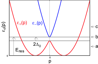
Figure 1: (Color online) Energy dispersions for the Hamiltonian $\hat{H}_{0}$ in Eq. (2).

On the other hand, adiabatic semi-classical Boltzmann transport analyses suggest that impurity scattering produces the AHE through the “skewness” Smit55 ; Luttinger58 ; Nozieres73 or the side jump Berger70 ; Nozieres73 . The skew-scattering contribution diverges in the clean limit as $\sigma_{xy}^{\rm skew}=\sigma_{xx}S=\frac{2e^{2}}{ha}\frac{E_{F}\tau}{\hbar}S$ with the life time $\tau$ and the Fermi energy $E_{F}$. Here, $S\sim\varepsilon_{SO}v_{\rm imp}/W^{2}(\ll 1)$ is the skewness factor with $W$ being the bandwidth or the inverse of the density of states and $v_{\rm imp}$ the impurity potential strength.

Generic model that fully takes into account both the “parity anomaly” associated with the anti-crossing of band dispersions and the impurity scattering can be obtained by expanding the Hamiltonian at a fixed $p_{z}$ with respect to the momentum $\bm{p}$ measured from the originally crossing point $\bm{p}_{0}$ of two dispersions;

$$\hat{H}_{0}+\hat{H}_{\text{imp}}=-\Delta_{0}\hat{\sigma}^{z}+v\bm{p}\cdot\hat{\bm{\sigma}}\times\bm{e}^{z}+\frac{\bm{p}^{2}}{2m}+v_{\rm imp}\sum_{\bm{r}_{\rm imp}}\delta(\bm{r}-\bm{r}_{\rm imp})$$ (2)

with the position $\bm{r}$ of electron, the Pauli matrices $\hat{\bm{\sigma}}=(\hat{\sigma}_{x},\hat{\sigma}_{y},\hat{\sigma}_{z})$, the unit vector $\bm{e}^{z}$ in the $z$ direction, and an impurity at a position $\bm{r}_{\rm imp}$. The first term corresponds to the level splitting $2\Delta_{0}=\varepsilon_{SO}$ of two bands at the anti-crossing momentum. The second term gives the linear dispersion with the velocity $v$. The third term represents the quadratic dispersion with an effective mass $m$, whose anisotropy has been neglected since it is unimportant. This model has two band dispersions $\varepsilon_{\pm,\bm{p}}$ as shown in Fig. 1. Henceforth, the bottom of the lower band is chosen as the origin of the energy and the bottom of the upper band denoted as $E_{\rm res}=\varepsilon_{-}(0)$ is taken as an energy unit. The model possesses the gauge flux $b^{z}_{\pm,\bm{p}}=\mp\lambda^{2}\Delta_{0}/2\Delta_{\bm{p}}^{3}$ with $\Delta_{\bm{p}}=\sqrt{\lambda^{2}\bm{p}^{2}+\Delta_{0}^{2}}$ Dugaev05 ; Sinitsyn05 . In the case of resonance, $E_{F}\in[E_{\rm res}-2\Delta_{0},E_{\rm res}]$, $\sigma_{xy}^{TKNN}$ approaches the maximum value $e^{2}/2h$. Away from this resonance, dominant contributions from the momentum region around $\bm{p}=0$ cancel out each other or do not appear, leading to a suppression of $\sigma_{xy}^{TKNN}(\approx(e^{2}/h)(\varepsilon_{SO}/E_{F}))$, where the perturbation expansion in $\varepsilon_{SO}$ is justified. Therefore, the present model, Eq. (2), can be regarded as a generic continuum model for a momentum region that gives a major contribution to the AHE. By definition of the anti-crossing, $\Delta_{0}$ does not change its sign as a function of $p_{z}$. This removes a concern that the integration over $p_{z}$ might lead to a cancellation.

We employ the Keldysh formalism for non-equilibrium Green’s functions, which has recently been reformulated for generic multi-component systems Onoda06 . We consider Green’s functions and self-energies under an applied constant electric field $\bm{E}=(0,E_{y})$; $\hat{G}^{\alpha}(\varepsilon,\bm{p})$ and $\hat{\Sigma}^{\alpha}(\varepsilon)$ with $\alpha=R,A,<$ for the retarded, advanced and lesser components, respectively. $\varepsilon$ and $\bm{p}$ represent the covariant energy and momentum in the Wigner representation Onoda06 . $\hat{G}^{\alpha}(\varepsilon,\bm{p})$ and $\hat{\Sigma}^{\alpha}(\varepsilon)$ can be expanded in $E_{y}$ as

$$\hat{G}^{\alpha}(\varepsilon,\bm{p}) = \hat{G}^{\alpha}_{0}(\varepsilon,\bm{p})+e\hbar E_{y}\hat{G}^{\alpha}_{E_{y}}(\varepsilon,\bm{p})+O(E_{y}^{2}),$$ (3)

$$\hat{\Sigma}^{\alpha}(\varepsilon) = \hat{\Sigma}^{\alpha}_{0}(\varepsilon)+e\hbar E_{y}\hat{\Sigma}^{\alpha}_{E_{y}}(\varepsilon)+O(E_{y}^{2}).$$ (4)

Henceforth, functionals with the subscripts 0 and $E_{y}$ denote those in the absence of and the gauge-invariant linear response to $E_{y}$. Due to the $\delta$-functional form of the impurity potential, the self-energies are local. $\hat{G}^{R,A}_{0}$ satisfies the familiar Dyson equation,

$$\hat{G}^{R,A}_{0}(\varepsilon,\bm{p})=[\varepsilon-\hat{H}_{0}(\bm{p})-\hat{\Sigma}^{R,A}_{0}(\varepsilon)]^{-1}.$$ (5)

The self-consistent equations for $\hat{G}^{R,A,<}_{E_{y}}$ are obtained by expanding the Dyson equation in the electric field Onoda06 . It is convenient to decompose $\hat{G}^{<}_{E_{y}}$ and $\hat{\Sigma}^{<}_{E_{y}}$ into two;

$$\hat{G}^{<}_{E_{y}}(\varepsilon,\bm{p}) = \hat{G}^{<}_{E_{y},I}(\varepsilon,\bm{p})\partial_{\varepsilon}f(\varepsilon)+\hat{G}^{<}_{E_{y},II}(\varepsilon,\bm{p})f(\varepsilon)$$ (6)

$$\hat{\Sigma}^{<}_{E_{y}}(\varepsilon) = \hat{\Sigma}^{<}_{E_{y},I}(\varepsilon)\partial_{\varepsilon}f(\varepsilon)+\hat{\Sigma}^{<}_{E_{y},II}(\varepsilon)f(\varepsilon)$$ (7)

$$\hat{G}^{<}_{E_{y},II}(\varepsilon,\bm{p}) = \hat{G}^{A}_{E_{y}}(\varepsilon,\bm{p})-\hat{G}^{R}_{E_{y}}(\varepsilon,\bm{p})$$ (8)

$$\hat{\Sigma}^{<}_{E_{y},II}(\varepsilon) = \hat{\Sigma}^{A}_{E_{y}}(\varepsilon)-\hat{\Sigma}^{R}_{E_{y}}(\varepsilon).$$ (9)

$\hat{G}^{<}_{E_{y},I}$ and $\hat{\Sigma}^{<}_{E_{y},I}$ can be self-consistently determined from the quantum Boltzmann equation in the first order in $E_{y}$,

$$\left[\hat{G}^{<}_{E_{y},I},\hat{H}_{0}\right]+\hat{G}^{<}_{E_{y},I}\hat{\Sigma}^{A}_{0}-\hat{\Sigma}^{R}_{0}\hat{G}^{<}_{E_{y},I}$$ (10)

$$=\hat{\Sigma}^{<}_{E_{y},I}\hat{G}^{A}_{0}-\hat{G}^{R}_{0}\hat{\Sigma}^{<}_{E_{y},I}-\frac{i}{2}\left[\hat{v}_{y},\hat{G}^{A}_{0}-\hat{G}^{R}_{0}\right]_{+}$$

$$+\frac{i}{2}\left((\hat{\Sigma}^{A}_{0}-\hat{\Sigma}^{R}_{0})(\partial_{p_{y}}\hat{G}^{A}_{0})+(\partial_{p_{y}}\hat{G}^{R}_{0})(\hat{\Sigma}^{A}_{0}-\hat{\Sigma}^{R}_{0})\right)$$

with the velocity $\hat{v}_{i}(\bm{p})=\partial_{p_{i}}\hat{H}_{0}(\bm{p})$, while $\hat{G}^{R,A}_{E_{y}}$ and $\hat{\Sigma}^{R,A}_{E_{y}}$ are determined from the other self-consistent equation,

$$\hat{G}^{R,A}_{E_{y}}=\hat{G}^{R,A}_{0}\hat{\Sigma}^{R,A}_{E_{y}}\hat{G}^{R,A}_{0}$$ (11)

$${}-\frac{i}{2}\left(\hat{G}^{R,A}_{0}\hat{v}_{y}(\partial_{\varepsilon}\hat{G}^{R,A}_{0})-(\partial_{\varepsilon}\hat{G}^{R,A}_{0})\hat{v}_{y}\hat{G}^{R,A}_{0}\right).$$

We can exactly calculate the self-energies $\hat{\Sigma}^{R,A}_{0}$ and $\hat{\Sigma}^{R,A,<}_{E_{y}}$ up to the $n_{\rm imp}$-linear terms by means of the $T$-matrix approximation;

$$\hat{\Sigma}^{R,A}_{0}(\varepsilon) = n_{\rm{imp}}\hat{T}^{R,A}_{0}(\varepsilon)$$ (12)

$$\hat{T}^{R,A}_{0}(\varepsilon) = v_{\rm{imp}}\left(1-v_{\rm imp}\int\frac{d^{2}\bm{p}}{(2\pi\hbar)^{2}}\hat{G}^{R,A}_{0}(\varepsilon,\bm{p})\right)^{-1}$$ (13)

for the zeroth-order in $E_{y}$ and

$$\hat{\Sigma}^{<}_{E_{y},I}(\varepsilon)\!\! = \!\!n_{\rm{imp}}\hat{T}^{R}_{0}(\varepsilon)\!\!\int\!\!\frac{d^{2}\bm{p}}{(2\pi\hbar)^{2}}\hat{G}^{<}_{E_{y},I}(\varepsilon,\bm{p})\hat{T}^{A}_{0}(\varepsilon)$$ (14)

$$\hat{\Sigma}^{R,A}_{E_{y}}(\varepsilon)\!\! = \!\!n_{\rm imp}\hat{T}^{R,A}_{0}(\varepsilon)\!\!\int\!\!\frac{d^{2}\bm{p}}{(2\pi\hbar)^{2}}\hat{G}^{R,A}_{E_{y}}(\varepsilon,\bm{p})\hat{T}^{R,A}_{0}(\varepsilon)$$ (15)

for the first-order in $E_{y}$. We solve Eqs. (5), (12) and (13) self-consistently to obtain $\hat{G}^{R,A}_{0}$ and $\hat{\Sigma}^{R,A}_{0}$. Next, they are plugged into Eqs. (10) and (14) to solve $\hat{G}^{<}_{E_{y},I}$ and $\hat{\Sigma}^{<}_{E_{y},I}$ self-consistently. $\hat{G}^{R,A}_{E_{y}}$ and $\hat{\Sigma}^{R,A}_{E_{y}}$ are obtained from Eqs. (11) and (15) , and hence $\hat{G}^{<}_{E_{y},II}$ through Eq. (8). The conductivity tensors are calculated from

$$\sigma_{ij}^{I}\!\! = \!\!-\frac{e^{2}\hbar}{2\pi i}\int\!\!\frac{d^{2}\bm{p}}{(2\pi\hbar)^{2}}{\rm Tr}\!\left[\hat{v}_{i}(\bm{p})\hat{G}^{<}_{E_{j},I}(\varepsilon,\bm{p})\right],$$ (16)

$$\sigma_{ij}^{II}\!\! = \!\!e^{2}\hbar\int\!\!\frac{d\varepsilon}{2\pi i}\int\!\!\frac{d^{2}\bm{p}}{(2\pi\hbar)^{2}}{\rm Tr}\!\left[\hat{v}_{i}(\bm{p})\hat{G}^{<}_{E_{j},II}(\varepsilon,\bm{p})\right]\!f(\varepsilon),$$ (17)

with $i,j=x,y$. Note that Eqs. (16) and (17) are along the same spirit as the Str̆eda formula Streda82 : this approach provides the diagrammatic treatment for the Str̆eda formula Onoda06 . Effects of the vertex corrections to $\hat{G}^{<}_{E_{j},II}$ cancel each other, and hence we can regard $\sigma_{xy}^{II}$ as an intrinsic contribution. By contrast, the Fermi-surface contribution $\sigma_{xy}^{I}$ suffers from a vertex correction. While the intra-band matrix elements correspond to the conventional description of both $\sigma_{xx}$ and $\sigma_{xy}$ based on the scattering events, the inter-band ones contain a finite intrinsic contribution to the AHE as a part of the Berry-curvature term Sinitsyn06 and is generically expressed as

$$\sigma^{I\ {\rm int}}_{ij}=-\epsilon_{ij\ell}\frac{e^{2}\hbar}{2}\int\!\frac{d\bm{p}}{(2\pi\hbar)^{d}}\sum_{n,n^{\prime}}(\varepsilon_{n}(\bm{p})-\varepsilon_{n^{\prime}}(\bm{p}))$$ (18)

$$\!\!\!\times\partial_{\varepsilon}f(\varepsilon_{n}(\bm{p})){\rm Im}\left(\langle n\bm{p}|\bm{\nabla}_{p}|n^{\prime}\bm{p}\rangle\times\langle n^{\prime}\bm{p}|\bm{\nabla}_{p}|n\bm{p}\rangle\right)_{\ell}.$$

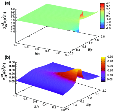
Figure 2: (Color) (a) The total anomalous Hall conductivity $\sigma_{xy}^{\rm tot}$ against $E_{F}$ and $\hbar/\tau$ in an energy unit of $E_{\rm res}=1.0$. (b) The intrinsic contribution $\sigma_{xy}^{\rm int}$ for the same parameter values. Note the difference of the scales for $\sigma_{xy}$ in (a) and (b).

Figure 2(a) shows the numerical results on $\sigma_{xy}^{\rm tot}=\sigma_{xy}^{I}+\sigma_{xy}^{II}$ against the Fermi energy $E_{F}$ and the Born scattering amplitude $\hbar/\tau\equiv n_{\rm imp}v_{\rm imp}^{2}m$ for a typical set of parameters, $\Delta_{0}=0.1$, $2mv_{\rm imp}=0.6$, $2m\lambda^{2}=3.59$, and the energy cutoff is taken as $E_{c}=3.0$ in an energy unit of $E_{\rm res}=1.0$ Inoue06 . In the clean limit $\hbar/\tau\to 0$, $\sigma_{xy}^{\rm tot}$ diverges in accordance with the skew-scattering scenario. Strength of the divergence is proportional to $E_{F}$ in the low electron-density limit, and the sign is inverted around $E_{F}=\varepsilon_{+}(0)=E_{\rm res}-2\Delta_{0}$. Sign of the skew-scattering contribution also changes by the sign change of $v_{\rm imp}$. Figure 2(b) shows the intrinsic contribution $\sigma_{xy}^{\rm int}$ calculated by imposing $\hat{\Sigma}^{R,A,E}_{E_{y}}=0$ for the same set of parameters. Under the resonant condition for $E_{F}$, $\sigma_{xy}^{\rm int}$ becomes of the order of $e^{2}/2h$. With increasing $\hbar/\tau$, it gradually decreases solely due to damping of quasi-particles.

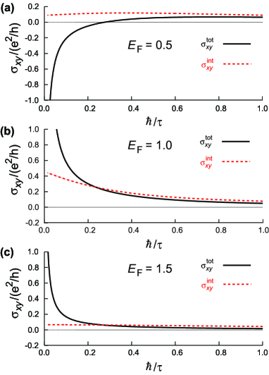
Figure 3: (Color online) $\sigma_{xy}^{\text{tot}}$ and $\sigma_{xy}^{\text{int}}$ as a function of $\hbar/\tau$ for the same parameter values as Fig. 2 with $E_{F}=0.5$, $1.0$ and $1.5$ for (a), (b), and (c), respectively.

By contrast, with increasing $\hbar/\tau$, the extrinsic skew-scattering contribution rapidly decays (Fig. 3), reflecting that it originates purely from intra-band processes and hence the skewness factor $S$ remains of the order of $\varepsilon_{SO}v_{\rm imp}/W^{2}$. In moderately dirty cases, the total conductivity nearly merges into the intrinsic value. Namely, there appears a crossover from the extrinsic regime to the intrinsic as $\hbar/\tau$ increases. Especially in the resonant case ($E_{F}=E_{\text{res}}$) shown in Fig. 3 (b), the intrinsic contribution is significantly enhanced and the extrinsic-to-intrinsic crossover occurs at $\hbar/\tau\sim\varepsilon_{SO}$. For a small ratio of $\varepsilon_{SO}/E_{F}\sim 10^{-3}-10^{-2}$ Fang03 ; Yao04 , dominance of the intirnsic AHE is realized within the usual clean metal. In reality, the total Hall conductivity is the sum of the contributions from all over the Brillouin zone. Since skew-scattering contributions from other momentum regions are always subject to a similar rapid decay, the above extrinsic-to-intrinsic crossover still occurs unless contributions from all the anti-crossing regions of band dispersions are mutually canceled out by accident.

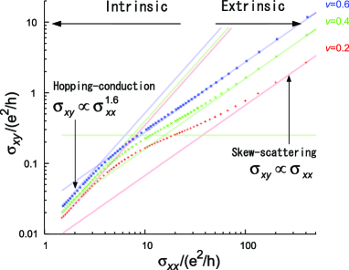
Figure 4: (Color online) Scaling plot of $\sigma_{xy}$ versus $\sigma_{xx}$ for the same sets of parameter values as in Fig. 3(b) except $2mv_{\rm imp}$.

Figure 4 shows the logarithmic plot of $\sigma_{xy}$ against $\sigma_{xx}$ for the same set of parameters as Fig. 3(b) except for the impurity scattering strength $v_{\rm imp}$, which is varied for different curves. In the clean limit, the curves nicely follow $\sigma_{xy}\propto\sigma_{xx}$ and the ratio $\sigma_{xy}/\sigma_{xx}$ is proportional to $v_{\rm imp}$ for a fixed $\tau$. As $\sigma_{xx}=2(e^{2}/h)E_{F}\tau/\hbar$ decreases with decrease in $\tau$, the relation exhibits a upward deviation from the linear one, signalling the crossover to the intrinsic regime. A smaller impurity potential strength $v_{\rm imp}$ enlarges the region of the constant behaviour of $\sigma_{xy}$. (Note that we change $n_{\rm imp}$ to control $\hbar/\tau$.) Careful experiments are required to test the prediction of the crossover at low temperatures. The magnitude of $\sigma_{xy}$ in the intrinsic regime is consistent with experimentally observed values $\sigma_{xy}\cong 10^{2}-10^{3}\ \Omega^{-1}{\rm cm}^{-1}$ in a $\sigma_{xy}$-constant region of Fe- and Ni-based dilute alloys Hurd , and SrRuO₃ and metallic foils Asamitsu . Further decrease of $\tau$ again changes the scaling behaviour to $\sigma_{xy}\propto\sigma_{xx}^{1.6}$, which almost agrees with recent experiments on a disordered pyrochlore ferromagnet Nd₂(Mo_1-xNb_x)₂O₇ Iguchi and on La_1-xSr_xCoO₃ Asamitsu . This exponent approximates to the value expected for the normal Hall effect in the hopping conduction regime PryadkoAuerbach04 .

Now the source of the confusion over decades is clear. The skew-scattering contribution, though it is rather sensitive to details of the impurity potential and band structure, can be larger than $e^{2}/h$ in the superclean case $\hbar/\tau\ll\varepsilon_{SO}$, but decays for $\varepsilon_{SO}<\hbar/\tau$. The side-jump contribution is smaller and of the order of $(e^{2}/h)(\varepsilon_{SO}/E_{F})$ Nozieres73 . Therefore, the intrinsic one, which is of the order of $e^{2}/h$ under the resonant condition, is dominant over a wide range of the scattering strength $\varepsilon_{SO}<\hbar/\tau<E_{F}$ (clean case). Although Luttinger reconsidered the Karplus-Luttinger theory KarplusLuttinger54 and gave an expansion of $\sigma_{xy}$ in $v_{\rm imp}$, including the skew-scattering contribution as well Luttinger58 , it fails to reveal the above crossover in the space of $E_{F}$, $\varepsilon_{SO}$ and $\hbar/\tau$.

In conclusions, we have shown that the AHE is determined by the intrinsic mechanism when (i) the Fermi level is located around an anti-crossing of band dispersions in the momentum space, (ii) consequently the magnitude of $\sigma_{xy}$ is comparable to $e^{2}/(ha)\sim 10^{3}\ \Omega^{-1}$ cm^-1, and (iii) the resistivity $\rho_{xx}$ is larger than $(ha/e^{2})(\varepsilon_{SO}/E_{F})\sim 1$-$10\ \mu\Omega\ {\rm cm}$. With these conditions, first-principle calculation can give an accurate prediction of $\sigma_{xy}$. The present work resolves a long standing controversy on the mechanism of the AHE in a whole region.

The authors are grateful to A. Asamitsu, T. Miyazato, S. Iguchi, R. Mathieu, and Y. Tokura for fruitful discussion and showing unpublished experimental data, and H. Fukuyama, A. H. MacDonald, J. Sinova, J. Inoue, S. Murakami, K. Nomura, and M. Onoda for stimulating discussion. Numerics was performed using the supercomputer at the Institute of Solid State Physics, University of Tokyo. The work was supported by Grant-in-Aids and NAREGI Nanoscience Project from the Ministry of Education, Culture, Sports, Science, and Technology.

References

• (1) C. M. Hurd, The Hall Effect in Metals and Alloys (Plenum Press, New York, 1972).
• (2) R. Karplus and J. M. Luttinger, Phys. Rev. 95, 1154 (1954).
• (3) J. Smit, Physica 21, 877 (1955).
• (4) L. Berger, Phys. Rev. B 2, 4559 (1970).
• (5) J. M. Luttinger, Phys. Rev. 112, 739 (1958).
• (6) J. Kondo, Prog. Theor. Phys. 27, 772 (1962).
• (7) P. Nozieres and C. Lewiner, J. Phys. (Paris) 34, 901 (1973).
• (8) H. Ohno, Sience 281, 951-956 (1998).
• (9) W.-L. Lee et al., Science 303, 1647 (2004).
• (10) N. Manyala et al., Nature Materials 3, 255 (2004).
• (11) R. E. Prange and S. M. Girvin, (eds.) The Quantum Hall Effect (Springer, Berlin, 1987).
• (12) P. Str̆eda, J. Phys. C: Solid State Phys. 15, L717 (1982).
• (13) D. J. Thouless et al., Phys. Rev. Lett. 49, 405 (1982).
• (14) G. Sundaram and Q. Niu, Phys. Rev. B 59, 14915 (1999).
• (15) M. Onoda and N. Nagaosa, J. Phys. Soc. Jpn. 71, 19 (2002).
• (16) T. Jungwirth, Q. Niu, and A. H. MacDonald, Phys. Rev. Lett. 88, 207208 (2002).
• (17) R. Jackiw, Phys. Rev. D 29, 2375 (1984).
• (18) Z. Fang et al., Science 302, 92 (2003).
• (19) Y. Yao et al., Phys. Rev. Lett. 92, 037204 (2004).
• (20) V. K. Dugaev et al., Phys. Rev. B 71, 224423 (2005).
• (21) N. A. Sinitsyn et al., Phys. Rev. B 72, 045346 (2005).
• (22) S. Onoda, N. Sugimoto, and N. Nagaosa, Prog. Theor. Phys. 116, 61 (2006), and references therein.
• (23) N. A. Sinitsyn et al., cond-mat/0602598.
• (24) Non-scalar relaxation rate leads to $\sigma_{xy}\neq 0$ even for $E_{F}>E_{\text{res}}$ [J. Inoue et al., cond-mat/0604108].
• (25) T. Miyazato et al., private communication.
• (26) S. Iguchi et al., private communication.
• (27) L. P. Pryadko and A. Auerbach, Phys. Rev. Lett. 82, 1253 (2004).