Phases of a polar spin-1 Bose gas in a magnetic field

Abstract

The two Bose–Einstein condensed phases of a polar spin-1 gas at nonzero magnetizations and temperatures are investigated. The Hugenholtz–Pines theorem is generalized to this system. Crossover to a quantum phase transition is also studied. Results are discussed in a mean field approximation.

Bose–Einstein condensed spin-1 gases have rich magnetic properties Stenger et al. (1999); Stamper-Kurn and Ketterle (2001); Gu and Klemm (2003); Kis-Szabó et al. (2005); Szirmai et al. (2005). They can be classified according to the sign of the spin-dependent part of the interaction. In this paper this sign is assumed to be positive, i.e. the interaction is of antiferromagnetic type. In the absence of a magnetic field the system at zero temperature is in the polar state Ho (1998); Ohmi and Machida (1998) and no spontaneous magnetization is created. An external magnetic field induces a magnetization and as shown by Ohmi and Machida Ohmi and Machida (1998) in the Bogoliubov approximation a complete spin order appears when the magnetic field is strong enough.

The purpose of the present paper is to extend the investigations for a homogeneous system to finite temperatures below the Bose–Einstein condensation (BEC). We shall denote by P2 the phase originated from the polar state when a small magnetic field is switched on. This phase goes over to another one denoted by P1 when the magnetic field $B$ and/or the temperature is raised. In the P2 phase two continuous symmetries are broken while in phase P1 only one. The ground state spinor has two and one components, respectively. Correspondingly, two gapless (Goldstone) modes are expected to exist in P2. One of them develops a gap when entering the phase P1. Extended Hugenholtz–Pines theorems will be presented whose fulfilment is a necessary condition for such a behaviour. Another interesting aspect of this phase transition is the crossover from a classical to a quantum phase transition when the temperature goes to zero, which will also be investigated. Furthermore as in Stenger et al. (1999); Stamper-Kurn and Ketterle (2001) a nonzero magnetic chemical potential $\mu_{m}$ is included in the treatment. The discussion above remains valid, if the magnetic field $B$ were replaced by $\tilde{B}=B+\mu_{m}$, which can be regarded as an effective field determining the magnitude of the average magnetization.

For demonstration we choose a model which bears many features of the full microscopic description. As a matter of fact, it has been found in the case of a scalar Bose gas that the dielectric formalism can serve as a guide to find approximations which meet conservation laws and ensure that excitation branches associated with Goldstone modes are gapless Griffin (1993); Fliesser et al. (2001). Such an approach will be adopted here in a necessarily extended form since collective motions now include different types of spin waves besides particle density oscillations. Further differences arise due to the presence of the effective magnetic field $\tilde{B}$. Different regions are distinguished in the model on the $\tilde{B}-T$ plane. Properties are discussed particularly in those regions, which might be experimentally accessible (note that the theory worked out for a homogeneous system can be applied for a large system as a local density approximation).

We consider a translationally invariant system of spin-1 particles in a box with volume $V$ in a homogeneous, external magnetic field pointing to the z-direction. The Hamiltonian takes the following form:

$${\mathcal{H}}=\sum_{\genfrac{}{}{0.0pt}{2}{{\mathbf{k}}}{r,s}}\Big{[}(e_{{\mathbf{k}}}-\mu)\delta_{rs}-\hslash\tilde{\omega}_{\mathrm{L}}\,(F_{z})_{rs}\Big{]}a_{r}^{\dagger}({\mathbf{k}})a_{s}({\mathbf{k}})\\ +\frac{1}{2V}\sum_{\genfrac{}{}{0.0pt}{2}{{\mathbf{k}}_{1}+{\mathbf{k}}_{2}={\mathbf{k}}_{3}+{\mathbf{k}}_{4}}{r,s,r^{\prime},s^{\prime}}}a^{\dagger}_{r^{\prime}}({\mathbf{k}}_{1})a^{\dagger}_{r}({\mathbf{k}}_{2})V^{r^{\prime}s^{\prime}}_{rs}a_{s}({\mathbf{k}}_{3})a_{s^{\prime}}({\mathbf{k}}_{4}),$$ (1)

where $a_{r}^{\dagger}({\mathbf{k}})$ and $a_{r}({\mathbf{k}})$ are creation and destruction operators, respectively, of one-particle plane wave states with momentum ${\mathbf{k}}$ and spin projection $r$. The spin index $r$ refers to the eigenvalue of the z-component of the spin operator and can take the values $+,0,-$. Summation over repeated indices is understood throughout the paper. In this usual basis the spin operators are given by $F_{z}=\mathrm{diag}(1,0,-1)$ and $F_{x}=(F_{+}+F_{-})/2$ and $F_{y}=(F_{+}-F_{-})/2i$, and finally: $F_{\pm}=\sqrt{2}(\delta_{r,\pm}\delta_{s,0}+\delta_{r,0}\delta_{s,\mp})$. In Eq. (1) $e_{{\mathbf{k}}}=\hslash^{2}k^{2}/2M$ refers to the kinetic energy of an atom ($M$ is the mass of an atom), $\mu$ denotes the chemical potential. The quantities $\tilde{B}$ and $\tilde{\omega}_{\mathrm{L}}$ are introduced as

$$g\mu_{\mathrm{B}}\tilde{B}\equiv\hslash\tilde{\omega}_{\mathrm{L}}=\hslash\omega_{\mathrm{L}}+g\mu_{B}\mu_{m}.$$ (2)

Here $\hslash\omega_{\mathrm{L}}$ is the Zeeman energy shift in a magnetic field: $\hslash\omega_{\mathrm{L}}=g\mu_{\mathrm{B}}B$, where $g$ is the gyromagnetic ratio, $\mu_{\mathrm{B}}$ is the Bohr magneton; $B$ is the modulus of the homogeneous magnetic field and $\mu_{m}$ plays the role of a Lagrange multiplier for the magnetization. In Eq. (1) $V^{r^{\prime}s^{\prime}}_{rs}$ is the Fourier transform of the two particle interaction potential, which for the low temperature, dilute gas can be modeled by the momentum independent amplitude given for spin-1 bosons by Ho (1998); Ohmi and Machida (1998); Stamper-Kurn and Ketterle (2001):

$$V^{r^{\prime}s^{\prime}}_{rs}=c_{n}\delta_{rs}\delta_{r^{\prime}s^{\prime}}+c_{s}({\mathbf{F}})_{rs}({\mathbf{F}})_{r^{\prime}s^{\prime}},$$ (3)

In this paper we consider systems with $c_{s}>0$. An example of such a system is the gas of ${}^{23}\mathrm{Na}$ atoms Crubellier et al. (1999).

It is important that preparing the system with a suitable magnetization the effective field $\tilde{B}$ can be made much smaller than the external magnetic field $B$. This procedure made possible to observe experimentally the phase P2 (see Fig. 3c in Ref. Stenger et al. (1999) and Figs. 21c, 22c in Ref. Stamper-Kurn and Ketterle (2001)). Note that the quadratic Zeemann shift makes the phases P1 and P2 unstable for increasing magnetic field. It is assumed throughout this paper that the system is away from this stability border and the condensation occurs only in the spin directions $+$ and $-$.

The Hamiltonian (1) is invariant under the gauge transformations $a_{\pm}\rightarrow a_{\pm}e^{i\varphi_{\pm}}$ and $a_{0}\rightarrow a_{0}e^{i\frac{1}{2}(\varphi_{+}+\varphi_{-})}$. This is equivalent to $a_{r}\rightarrow a_{r}e^{i(\phi+r\varphi)}$, with $\phi=(\varphi_{+}+\varphi_{-})/2$ and $\varphi=(\varphi_{+}-\varphi_{-})/2$. The invariance under transformations with $\varphi\equiv 0$ yields a conservation law for the particle number, while with $\phi\equiv 0$ results in the conservation of the z-component of total magnetization.

We investigate such a parameter region $(\mu,\tilde{B},T)$, where the system has a Bose–Einstein condensate $\left<a_{r}({\mathbf{0}})\right>=\sqrt{N_{\text{c}}}\zeta_{r}$, with $N_{\text{c}}$ the number of atoms in the condensate and $\zeta_{r}=(\zeta_{+},\zeta_{0},\zeta_{-})$ being the normalized spinor of the condensate Ho (1998). One can take $\zeta_{0}=0$, which can be shown to be consistent with the general theory, i.e. to all orders in the perturbation expansion. Note that when the magnetic field and the magnetization are zero the magnitudes of the two components of the spinor ($\zeta_{+}$ and $\zeta_{-}$) are equal. This spinor is equivalent to what is usually taken for the polar state, i.e. $\zeta=(0,1,0)$ Ho (1998). It is convenient to define a new set of creation and annihilation operators: $b_{r}({\mathbf{k}})\equiv a_{r}({\mathbf{k}})-\sqrt{N_{\text{c}}}\zeta_{r}\delta_{{\mathbf{k}},0}$ and consider the Hamiltonian (1) as expressed with this new set. The canonical transformation, together with the requirement

$$\left<b_{r}({\mathbf{k}})\right>=\left<b^{\dagger}_{r}({\mathbf{k}})\right>=0$$ (4)

let us to define an ensemble with density matrix $\rho=\exp(-\beta\mathcal{H})/Z$ that exhibits the symmetry breaking associated with Bose–Einstein condensation.

The general features of the phase diagram can be read in Fig. 1 (calculated in an approximation to be introduced in the second part of the paper). The red line designates the border for BEC of the spin-1 gas, $T_{\mathrm{c}}$ denoting the critical temperature at $\tilde{B}=0$. In phase P2 the condensate is characterized by a two component spinor $\zeta=(\zeta_{+},0,\zeta_{-})$, $|\zeta_{+}|^{2}+|\zeta_{-}|^{2}=1$, while in P1 $\zeta=(1,0,0)$. For the P2–P1 phase transition the order parameter is $\sqrt{N_{\text{c}}}\zeta_{-}$. In the P2 phase both symmetries expressing the conservation of the particle number and that of the z-component of the magnetization are broken by fixing $\varphi_{+}$ and $\varphi_{-}$. In the P1 phase like in the ferromagnetic case Ho (1998) the only remaining phase $\varphi_{+}$ is related to the breaking of the combined symmetry of particle number conservation and magnetization.

The key quantity in our presentation is the finite-temperature Green’s function of the system:

$$\mathcal{G}^{rs}_{\gamma\delta}({\mathbf{k}},\tau)=-\Big{<}T_{\tau}\big{[}b^{\gamma}_{r}({\mathbf{k}},\tau)b^{\delta^{\dagger}}_{s}({\mathbf{k}},0)\big{]}\Big{>}.$$ (5)

$\tau$ is the imaginary time and $T_{\tau}$ refers to the $\tau$ ordering operator Shi and Griffin (1998); Griffin (1993). The Greek indices take the values $\pm 1$, with $b^{\gamma}_{r}({\mathbf{k}})=b_{r}({\mathbf{k}})$ if $\gamma=1$ and $b^{\gamma}_{r}({\mathbf{k}})=b_{r}^{\dagger}(-{\mathbf{k}})$ if $\gamma=-1$. Here $\mathcal{G}^{rs}_{1,1}({\mathbf{k}},\tau)$ and $\mathcal{G}^{rs}_{-1,-1}({\mathbf{k}},\tau)$ stand for the normal Green’s functions, while $\mathcal{G}^{rs}_{1,-1}({\mathbf{k}},\tau)$ and $\mathcal{G}^{rs}_{-1,1}({\mathbf{k}},\tau)$ for the anomalous ones, which arise due to Bose–Einstein condensation.

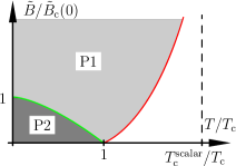
Figure 1: The phase diagram of the antiferromagnetic spin-1 Bose gas obtained in the mean field approximation

The propagator $\mathcal{G}^{00}_{\gamma\delta}$ describes dynamics corresponding to rotations around axes lying in the $x$-$y$ plane. Such spin-wave modes have a gap due to the nonzero effective magnetic field $\tilde{B}$. One can convince oneself, that the specific choice of the spinor, i.e. $\zeta_{0}=0$, and of the direction of the magnetic field leads to $\mathcal{G}^{rs}_{\gamma\delta}=0$ for $r=0$ ($s=0$) and $s=\pm$ ($r=\pm)$. As a consequence $\mathcal{G}^{00}_{\gamma\delta}$ decouples from the other Green’s functions and will not be discussed here further since we concentrate on the order parameter related to the P1–P2 transition and to its correlations described by $\mathcal{G}^{--}_{\gamma\delta}$.The structure and couplings of the Green’s function $\mathcal{G}^{--}_{\gamma\delta}$ are different in the phases P1 and P2. The main results are as follows.

In P2 $\mathcal{G}^{--}_{\gamma\delta}$ is coupled to $\mathcal{G}^{++}_{\gamma\delta}$ by $\mathcal{G}^{+-}_{\gamma\delta}$. The $4\times 4$ matrix with elements $\mathcal{G}^{rs}_{\gamma\delta}$, $r,s=\pm$ denoted by $\underline{\underline{\mathcal{G}}}$ takes the form in the Matsubara representation

$$\underline{\underline{\mathcal{G}}}^{-1}({\mathbf{k}},i\omega{{}_{n}})=\underline{\underline{\mathcal{G}}}{}_{(0)}^{-1}({\mathbf{k}},i\omega{{}_{n}})-\underline{\underline{\Sigma}}({\mathbf{k}},i\omega{{}_{n}}),$$ (6)

with the self-energy given by the following hypermatrix notation:

$$\underline{\underline{\Sigma}}=\left[\begin{array}[]{l r}\underline{\Sigma}^{++}&\underline{\Sigma}^{+-}\\ \underline{\Sigma}^{-+}&\underline{\Sigma}^{--}\end{array}\right],\quad\underline{\Sigma}^{rs}=\left[\begin{array}[]{l r}\Sigma^{rs}_{1,1}&\Sigma^{rs}_{1,-1}\\ \Sigma^{rs}_{-1,1}&\Sigma^{rs}_{-1,-1}\end{array}\right].$$ (7)

The inverse of the free propagator is $\underline{\underline{\mathcal{G}}}{}_{(0)}^{-1}=\mathrm{diag}(\Xi+\tilde{\omega}_{\mathrm{L}},\Xi^{*}+\tilde{\omega}_{\mathrm{L}},\Xi-\tilde{\omega}_{\mathrm{L}},\Xi^{*}-\tilde{\omega}_{\mathrm{L}})$, with $\Xi=i\omega_{n}-\hslash^{-1}(e_{{\mathbf{k}}}-\mu)$. The asterisk denotes complex conjugation.

Concerning the related spectrum it is important that the two components of the condensate are independent in the sense that they have independent phases: $\zeta^{\prime}=(e^{i\varphi_{+}}\zeta_{+},0,e^{i\varphi_{-}}\zeta_{-})$ is equivalent to $\zeta=(\zeta_{+},0,\zeta_{-})$. Consequently two gapless Goldstone modes are expected. In this respect it is important that generalized Hugenholtz–Pines (GHP) theorems are valid. They are as follows

$$\Sigma^{++}_{1,1}({\mathbf{0}},0)-\Sigma^{++}_{1,-1}({\mathbf{0}},0)=\hslash^{-1}\mu+\tilde{\omega}_{\mathrm{L}},$$ (8a)

$$\Sigma^{--}_{1,1}({\mathbf{0}},0)-\Sigma^{--}_{1,-1}({\mathbf{0}},0)=\hslash^{-1}\mu-\tilde{\omega}_{\mathrm{L}},$$ (8b)

$$\Sigma^{+-}_{1,1}({\mathbf{0}},0)-\Sigma^{+-}_{1,-1}({\mathbf{0}},0)=0,$$ (8c)

One can show that these relations provide necessary conditions for the existence of gapless modes, since the denominator of the Green’s function matrix as defined in Eq. (6) is zero at $k=0$, $i\omega_{n}=0$ if Eqs. (8) are fulfilled.

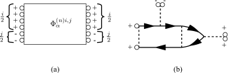
Figure 2: (a) The symbolic representation of an irreducible diagram having $i$ condensate lines with $r=+$ and $j$ with $r=-$. (b) A fourth order example is shown with $i=4$ and $j=2$. The dashed line represents the interaction, the circle stands for the square root of the corresponding condensate density and the line with an arrow denotes the free Green’s function.

We sketch the derivation, because it sheds light on the structure of the perturbation expansion. Namely, all $n^{\text{th}}$ order diagrams contributing to the self-energies $\Sigma^{rs}_{11}({\mathbf{0}},0)$ and $\Sigma^{rs}_{1,-1}({\mathbf{0}},0)$ can be obtained easily from the one-particle irreducible graphs without external lines but with $i$ number of condensate lines with spin projection $+$ and $j$ number of condensate lines with spin projection $-$. Particle number and spin conservation results in $i$ and $j$ being even. For an illustration of such a graph see Fig. 2, where the condensate lines are represented by circles. Let us denote its contribution by $\Phi^{(n)i,j}_{\alpha}$. Here $n$ refers to the order in perturbation theory and the index $\alpha$ is for distinguishing between graphs with the same $n,i,j$ but different topologies and consequently different contributions. To obtain the $n^{\text{th}}$ order contribution of the normal self-energy $\Sigma^{++}_{11}({\mathbf{0}},0)$ one has to replace two appropriately chosen condensate lines by an incoming and an outgoing particle line. Note that those circles where incoming lines can be substituted are gathered at the left side of Fig. 2 (a) while those standing for possible places of outgoing lines at the right side. Finally one arrives at

$$\Sigma^{++}_{11}({\mathbf{0}},0)=\frac{1}{n_{\text{c,+}}}\sum_{i}\sum_{\alpha}\bigg{(}\frac{i}{2}\bigg{)}^{2}\Phi^{(n)i,j}_{\alpha},$$ (9)

where $n_{\text{c},r}=N_{\text{c}}|\zeta_{r}|^{2}/V$ is the condensate density in spin projection $r\in\{+,-\}$. For obtaining the anomalous $\Sigma^{++}_{1-1}({\mathbf{0}},0)$ self-energy one has to replace two appropriately chosen condensate lines by two outgoing lines. One gets that

$$\Sigma^{++}_{1,-1}({\mathbf{0}},0)=\frac{1}{n_{\text{c,+}}}\sum_{i}\sum_{\alpha}\bigg{(}\frac{i}{2}\bigg{)}\bigg{(}\frac{i}{2}-1\bigg{)}\Phi^{(n)i,j}_{\alpha}.$$ (10)

It is possible to calculate this way the contribution of the irreducible tadpole diagrams as well, i.e. those with one incoming particle line:

$$\Sigma^{+}_{0}=\frac{1}{\sqrt{n_{\text{c,+}}}}\sum_{i}\sum_{\alpha}\bigg{(}\frac{i}{2}\bigg{)}\Phi^{(n)i,j}_{\alpha}.$$ (11)

Using Eqs. (9), (10) and (11) one arrives at

$$\Sigma^{++}_{11}({\mathbf{0}},0)-\Sigma^{++}_{1,-1}({\mathbf{0}},0)=\frac{1}{\sqrt{n_{\text{c,+}}}}\Sigma^{+}_{0}.$$ (12)

The requirement formulated in Eq. (4) for $r=+$ is satisfied when $\Sigma^{+}_{0}=\hslash^{-1}\mu+\tilde{\omega}_{\mathrm{L}}$, that yields with (12) one of the GHP theorems (8a). One can prove the others similarly.

Crossing the border line one enters the P1 phase where the condensate spinor has only one nonzero component $\zeta=(1,0,0)$. This spinor has only one phase, which can be chosen freely; a continuous symmetry is restored and therefore only one Goldstone mode exists. Furthermore in phase P1 $\Sigma^{+-}_{\alpha\gamma}=\Sigma^{-+}_{\alpha\gamma}=0$. Consequently $\mathcal{G}^{++}_{\alpha\gamma}$ and $\mathcal{G}^{--}_{\alpha\gamma}$ are no more coupled. The remaining Goldstone mode shows up in the spectrum of $\mathcal{G}^{++}_{\alpha\gamma}$ and the HP theorem $\Sigma^{++}_{1,1}({\mathbf{0}},0)-\Sigma^{++}_{1,-1}({\mathbf{0}},0)=\hslash^{-1}\mu+\tilde{\omega}_{\mathrm{L}}$ ensures its gapless nature. The order parameter dynamics as described by $\mathcal{G}^{--}_{\alpha\gamma}$ further simplifies into

$$[\mathcal{G}^{--}_{11}({\mathbf{k}},i\omega{{}_{n}})]^{-1}=i\omega_{n}-\hslash^{-1}(e_{{\mathbf{k}}}-\mu+\hslash\tilde{\omega}_{\mathrm{L}})-\Sigma^{--}_{11},$$ (13)

since $\Sigma^{--}_{1,-1}=0$ Kis-Szabó et al. . The excitation spectrum determined by Eq. (13) has a gap, which disappears when reaching the phase boundary between P1 and P2:

$$\hslash\tilde{\omega}_{\mathrm{L}}^{\mathrm{c}}=\mu-\hslash\Sigma^{--}_{11}({\mathbf{0}},0)\big{|}_{\tilde{\omega}_{\mathrm{L}}=\tilde{\omega}_{\mathrm{L}}^{\mathrm{c}}}.$$ (14)

At $T=0$ this condition designates a quantum phase transition and it is expected that there is a crossover from classical to quantum phase transition when $T\rightarrow 0$ Sondhi et al. (1997). One can define the shift exponent $\phi_{\text{s}}$ by the equation $\tilde{B}_{\mathrm{c}}(T)=\tilde{B}_{\mathrm{c}}(0)-wT^{1/\phi_{\text{s}}}$ Fisher (1974). It is useful then to introduce the variable $x=T/[\tilde{B}-\tilde{B}_{\mathrm{c}}(0)]^{\phi_{\text{s}}}$. Denoting by $x_{\text{c}}$ its value on the critical line, one can write the leading singularities as follows

$$\mathcal{G}^{--}_{11}({\mathbf{0}},0) =\frac{C(T)}{\left|x-x_{\text{c}}\right|^{\gamma}},\quad T>0,$$ (15)

$$=\frac{Q}{\left|\tilde{B}-\tilde{B}_{\mathrm{c}}(0)\right|^{\gamma_{0}}},\quad T=0.$$

One can show that $\phi_{\text{s}}$ agrees with the usually defined crossover exponent $\phi$ when crossover scaling is valid [in this case $C(T)\sim T^{-\gamma_{0}/\phi}$ in Eq. (15)]. One can specify a low temperature region where the energy gap is higher than the temperature. Here only exponentially small corrections due to nonzero temperatures are expected.

In the following we will discuss static and dynamic properties within a kind of a mean field approach. We start by writing self-consistent equations for the densities of the conserved quantities

$$n =n_{\text{c,+}}+n_{\text{c,-}}+n^{\prime}_{+}+n^{\prime}_{0}+n^{\prime}_{-},$$ (16a)

$$m =n_{\text{c,+}}-n_{\text{c,-}}+n^{\prime}_{+}-n^{\prime}_{-},$$ (16b)

with $n$ being the total particle density and $m$ the magnetization density. The density of non-condensed atoms in spin projection $s\in\{+,0,-\}$ is given by the Bose distribution $n^{\prime}_{s}=V^{-1}\sum_{{\mathbf{k}}}n^{\prime}_{{\mathbf{k}},s}$, with $n^{\prime}_{{\mathbf{k}},s}=(e^{\beta\epsilon_{{\mathbf{k}},s}}-1)^{-1}$ and

$$\epsilon_{{\mathbf{k}},s}=e_{{\mathbf{k}}}+c_{n}n-\mu+s(c_{s}m-\hslash\tilde{\omega}_{\mathrm{L}}).$$ (17)

There exists also a relation following from the requirement $\left<b_{+}({\mathbf{0}})\right>=0$, which provides the equation

$$\mu+\hslash\tilde{\omega}_{\mathrm{L}}=c_{n}n+c_{s}m.$$ (18a)

This equation holds both in the P1 and P2 phases. In phase P2 $$n_{0,-}\neq 0 \left<b_{-}({\mathbf{0}})\right>=0$$ and a second equation emerges from the requirement , which reads as

$$\mu-\hslash\tilde{\omega}_{\mathrm{L}}=c_{n}n-c_{s}m.$$ (18b)

Using Eqs. (16), (17), (18a) and (18b) one can get the form of the spinor in phase P2, which reads

$$\zeta_{\pm}=\left[\frac{1}{2}\left(1\pm\frac{\hslash\tilde{\omega}_{\mathrm{L}}}{c_{s}n_{c}}\right)\right]^{\frac{1}{2}},$$ (19)

where $n_{c}$ is the total density of the condensate.

The obtained phase diagram is depicted in Fig. 1. For the critical line one gets

$$\frac{\tilde{B}_{\text{c}}(T)}{\tilde{B}_{\text{c}}(0)}=1-\left(\frac{T}{T_{c}}\right)^{3/2},$$ (20)

with $T_{c}=(4\pi^{2}n)^{2/3}\hslash^{2}/(3\Gamma(3/2)\zeta(3/2))^{2/3}2Mk_{B}$ being the critical temperature at $\tilde{B}=0$. Therefore the shift exponent is $\phi_{\text{s}}=2/3$.

The second step is to express the Green’s functions in harmony with the equation of state as written above. It can be shown that the self-consistent nature of the equation of state and the existence of the condensate leads to RPA like contributions to the self-energies. To see that the procedure leads to a conserving approximation one needs to treat correlation functions of the density and spin density operators in detail, which goes beyond the scope of the present paper and will be published together with the dielectric formalism generalized to $\tilde{B}\neq 0$ Kis-Szabó et al. .

We consider the P1 phase first. Since $n_{\text{c,-}}=0$ in this phase the RPA like terms are not present in $\Sigma^{--}_{\gamma\delta}$ (we recall that $\Sigma^{+-}_{\gamma\delta}=0$ anyhow in P1). Consequently $\mathcal{G}^{--}_{11}=[i\omega_{n}-\hslash^{-1}\epsilon_{{\mathbf{k}},-}]^{-1}$ which after a somewhat lengthy calculation leads to (15) with $\gamma=2$ and $\gamma_{0}=1$ and furthermore to $C(T)\sim T^{-1}$. Further critical exponents have the values $\eta=\eta_{0}=0$, $\nu=1$, $\nu_{0}=1/2$. They are defined as follows: $\mathcal{G}^{--}_{11}({\mathbf{0}},0)\sim 1/k^{2-\eta}$ on the critical line, while $\mathcal{G}^{--}_{11}({\mathbf{0}},0)\sim 1/k^{2-\eta_{0}}$ at the quantum critical point; the correlation length $\xi\sim 1/|x-x_{c}|^{\nu}$ and $\xi\sim 1/|\tilde{B}-\tilde{B}_{\mathrm{c}}(0)|^{\nu_{0}}$ at $T>0$ and at $T=0$, respectively. The dispersion relation is real and parabolic with a gap, that vanishes at the phase boundary between P1 and P2. The gap exponent is $\nu z$ ($T>0$), $\nu_{0}z$ (T=0), where the dynamical scaling exponent $z=2$. Choosing a path towards the quantum critical point such that $[\tilde{B}-\tilde{B}_{\mathrm{c}}(0)]/T=\text{const}>0$, one obtains $\mathcal{G}^{--}_{11}({\mathbf{0}},0)\sim T^{-\nu_{0}z}$. The slope of the border line of the low temperature region [specified below Eq. (15)] is proportional to $1/c_{s}$ and is about 200 in the units of Fig. 1 by choosing the following realistic parameter values: $c_{n}=1.03\cdot 10^{-50}\mathrm{J\,m^{3}},c_{s}=3.21\cdot 10^{-52}\mathrm{J\,m^{3}}$ and the density ($4.6\cdot 10^{20}\mathrm{m}^{-3})$. The correction to the leading $1/T$ singularity has a weaker power law dependence on $1/T$ (in the model $T^{-1/2}$). This region, which is presumably experimentally accessible terminates at the line $\tilde{B}=\tilde{B}_{\mathrm{c}}(0)$ along with $\mathcal{G}^{--}_{11}({\mathbf{0}},0)\sim T^{-3/2}$. Note that while the power law behaviours are expected to be generally valid the exponents along the critical line are characteristic for the model. Namely, they are those of the spherical model. The reason is that the model can be formally derived by introducing $\sigma$ species of spin-1 bosons and taking the limit $\sigma\rightarrow\infty$ while the interaction parameters $c_{n}$, $c_{s}$ are going to zero as $1/\sigma$. Furthermore $B$, $\mu$ and $\mu_{m}$ remain of ${\mathcal{O}}(1)$.

In phase P2 the complete self-energy matrix (7) has to be treated. One obtains for the Green’s function Kis-Szabó et al.

$$\left(\underline{\underline{\mathcal{G}}}^{-1}\right)^{rs}_{\alpha\gamma}=\left(i\omega_{n}-\hslash^{-1}e_{{\mathbf{k}}}\right)\delta_{rs}\delta_{\alpha\gamma}\\ -\hslash^{-1}\sqrt{n_{\text{c},r}n_{\text{c},s}}(\mathcal{C}_{n}+rs\mathcal{C}_{s}),$$ (21)

for $r,s\in\{+,-\}$. The effective interactions are given by $\mathcal{C}_{n}({\mathbf{k}},i\omega{{}_{n}})=c_{n}/[1-3c_{n}\Pi_{(0)}({\mathbf{k}},i\omega{{}_{n}})]$, $\mathcal{C}_{s}({\mathbf{k}},i\omega{{}_{n}})=c_{s}/[1-2c_{s}\Pi_{(0)}({\mathbf{k}},i\omega{{}_{n}})]$. The polarization function $\Pi_{(0)}$ is the contribution of the bubble diagram of the free gas, since $\epsilon_{{\mathbf{k}},s}=e_{{\mathbf{k}}}$ in P2 as can be seen from Eqs. (17), (18a) and (18b) and reads as

$$\Pi_{(0)}({\mathbf{k}},i\omega{{}_{n}})=-\frac{1}{\hslash}\int\frac{{\mathrm{d}^{3}}q}{(2\pi)^{3}}\frac{n^{\prime}_{{\mathbf{k}}+{\mathbf{q}},s}-n^{\prime}_{{\mathbf{q}},s}}{i\omega_{n}-\hslash^{-1}(e_{{\mathbf{k}}+{\mathbf{q}}}-e_{{\mathbf{q}}})},$$ (22)

for all values of $s$. By writing $c_{n},c_{s}$ instead of $\mathcal{C}_{n},\mathcal{C}_{s}$ the Bogoliubov approximation of the Green’s functions is formally recovered. It is remarkable that the GHP theorems (8) are fulfilled in this model in such a way that simultaneously

$$\Sigma^{rs}_{\alpha\beta}({\mathbf{k}},0)=\Sigma^{rr}_{\alpha\alpha}({\mathbf{k}},0)\delta_{rs}\delta_{\alpha\beta},\qquad k\rightarrow 0.$$ (23)

Repeated indices are not summed in this equation. If (23) were true in general then it would mean a generalization of the results by Nepomnyashchiĭ and Nepomnyashchiĭ Nepomnyashchiĭ and Nepomnyashchiĭ (1978) derived at $T=0$ in the case of liquid Helium, i.e. for particles with zero spin. Namely, by analyzing the infrared divergences they have shown that the anomalous self-energy $\Sigma_{1,-1}({\mathbf{0}},0)=0$. At nonzero temperature the expected behaviour is that $\Sigma_{1,-1}({\mathbf{k}},0)\sim k$ Shi and Griffin (1998), which is valid here for all the nondiagonal self-energies, since $\Pi_{(0)}({\mathbf{k}},0)\sim k^{-1}$.

The denominator of the Green’s function (after analytical continuation in frequency) reads as:

$$\Delta({\mathbf{k}},\omega)=\big{[}\omega^{2}-\hslash^{-2}e_{{\mathbf{k}}}^{2}\big{]}^{2}(1-2c_{s}\Pi_{(0)}^{\text{ret}})(1-3c_{n}\Pi_{(0)}^{\text{ret}})\\ -2\hslash^{-2}e_{{\mathbf{k}}}\big{[}\omega^{2}-\hslash^{-2}e_{{\mathbf{k}}}^{2}\big{]}n_{\text{c}}(c_{n}+c_{s}-5c_{n}c_{s}\Pi_{(0)}^{\text{ret}})\\ +16\hslash^{-4}e_{{\mathbf{k}}}^{2}c_{n}c_{s}n_{\text{c,+}}n_{\text{c,-}}.$$ (24)

The spectrum of elementary excitations is given by $\Delta({\mathbf{k}},\omega)|_{\omega=E_{{\mathbf{k}}}-i\gamma_{{\mathbf{k}}}}=0$. Three correlation lengths will be used to specify regions in the phase diagram with qualitatively different solutions, namely the thermal wavelength $\lambda=\hslash/(2Mk_{\mathrm{B}}T)^{1/2}$, the Bogoliubov coherence length $\xi_{\text{B}}=\hslash/(4Mc_{s}n_{\text{c,-}})^{1/2}$, and the length characterizing phase fluctuations of the order parameter $\xi^{\prime}=Mk_{\mathrm{B}}T/(4\pi\hslash^{2}n_{\text{c,-}})$. The three regions of the phase P2 are illustrated in Fig 3. For the sake of simplicity we restrict the discussion to small $k$ values and assume that $c_{s}/c_{n}$ is small, that is the case in the experiment Stamper-Kurn and Ketterle (2001). Region A ($\lambda\gg\xi_{\text{B}},\xi^{\prime}$): The polarization function can be approximated as

$$\Pi_{(0)}^{\text{ret}}({\mathbf{k}},\omega)=\frac{2pe_{{\mathbf{k}}}}{\omega^{2}},$$ (25)

where $p=\Gamma(3/2)\zeta(3/2)/4\pi^{2}\lambda^{3}$. The excitation energies are linear in wavenumber: $\omega_{\pm}=c_{\pm}k$. Here $c_{+}^{2}=nc_{n}/M-4c_{s}n_{+}n_{-}/(nM)$ and $c_{-}^{2}=n_{0}c_{s}/M+4c_{s}n_{+}n_{-}/(nM)$, where $n_{r}=n_{\text{c},r}+n_{r}^{\prime}$. At $T=0$ the result reduces to that of Ohmi and Machida obtained using the equation of motion method Ohmi and Machida (1998). In the present approximation a damping appears only for nonzero temperature, and is exponentially small. In higher order a Beliaev type damping can arise (see Shi and Griffin (1998) for a detailed investigation of such a damping in case of a gas of spinless bosons). It is assumed that $\tilde{B}$ is large enough that the interesting region in P2 keep away from the critical line of BEC. Then $\omega_{+}$ does not exhibit any remarkable change when approaching the P2-P1 boundary and therefore only $\omega_{-}$ will be followed below. In region B ($\xi_{\text{B}}\gg\xi^{\prime},\lambda$) the polarization function is approximated as

$$\Pi_{(0)}^{\text{ret}}({\mathbf{k}},\omega)=-i\frac{\hslash}{2Mc_{s}}\frac{\xi^{\prime}}{\xi_{B}^{2}}\frac{k}{\omega}.$$ (26)

The velocity contains only the condensate densities

$$c_{-}^{2}=\frac{4n_{\text{c,+}}n_{\text{c,-}}}{n_{\text{c}}}\frac{c_{s}}{M}$$ (27a)

and the mode has a Landau type damping

$$\gamma_{\mathbf{k}}=\frac{Mc_{s}}{4\pi\hslash^{3}}\left[2+3\left(\frac{\hslash\tilde{\omega}_{\mathrm{L}}}{c_{s}n_{\text{c}}}\right)^{2}\right]k_{\mathrm{B}}Tk.$$ (27b)

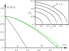
Figure 3: The three regions of the phase P2. Region A and C are enlarged for the sake of better visualization. The inset shows the order parameter as a function of temperature for several values of $\tilde{B}$.

Region C ($\xi^{\prime}\gg\xi_{\text{B}},\lambda)$ is the critical region. Here the polarization function $\Pi_{(0)}^{\text{ret}}({\mathbf{k}},i\omega{{}_{n}})$ takes the same form as in region B. For $\tilde{B},T$ fixed when $k\rightarrow 0$ the mode becomes overdamped and soft, $\omega_{-}=-i2\hslash k/(5M\xi^{\prime})$. For $k$ fixed $\omega_{-}$ tends to $e_{{\mathbf{k}}}$ when the critical line is approached. The size of these regions depends crucially on $c_{s}$ for the other parameters fixed. For realistic values of parameters the region A and C are very narrow, the region B is enlarged and experimentally accessible. Here the velocity depends on the condensate densities; the thermal excitations represent higher order corrections. More characteristically the damping is proportional to the wave number and the temperature. These features are known for density waves in Bose gases with frozen internal degrees of freedom Szépfalusy and Kondor (1974); Shi and Griffin (1998); Fliesser et al. (2001) and have been obtained also for spinor Bose gas at zero magnetization for the density (and spin density) fluctuations Szépfalusy and Szirmai (2002). The linear dependence on $T$ is even valid for gases in a magnetic trap Pitaevskii and Stringari (1997); Fedichev et al. (1998); Reidl et al. (2000). New feature of (27b) is the dependence on the strength of the magnetic field and magnetization. One expects that the leading term remains quadratic in $\tilde{B}$ also for a gas in an optical trap.

In conclusion, we have investigated the equilibrium and dynamic properties of the two Bose–Einstein condensed phases of a spin-1 Bose gas. The richness of properties of the two phases from the point of view of a many body problem is demonstrated by the GHP theorems. They reflect the basic fact that the number of Goldstone modes agrees with the independent phase fluctuations in the complex plane exhibited by the order parameter. One of them (in P2) is the critical mode for the P2–P1 transition, the other will become critical when the temperature in P1 reaches the line of BEC. The first mode (which coincides with the transverse spin wave only when the magnetization is zero) becomes a quadrupolar spin wave and develops a gap in P1. It has been shown that the transition between the phases P1 and P2 at zero temperature belongs to the category of quantum phase transitions in which a critical line starts from quantum critical point when the temperature is raised. The measurement of the shift exponent would be of particular interest.

The work was supported by the Hungarian National Research Foundation under Grant No. OTKA T046129.

References

Stenger et al. (1999)
J. Stenger,
S. Inouye,
D. M. Stamper-Kurn,
H.-J. Miesner,
A. P. Chikkatur,
and W. Ketterle,
Nature 396,
345 (1999).
Stamper-Kurn and Ketterle (2001)
D. Stamper-Kurn
and W. Ketterle,
in Les Houches, Session LXXII, Coherent atomic
matter waves, edited by
R. Kaiser,
C. Westbrook,
and F. David
(EDP Sciences; Springer-Verlag, Les
Ulis; Berlin, 2001), p. 137.
Gu and Klemm (2003)
Q. Gu and
R. A. Klemm,
Phys. Rev. A 68,
031604(R) (2003).
Kis-Szabó et al. (2005)
K. Kis-Szabó,
P. Szépfalusy,
and G. Szirmai,
Phys. Rev. A 72,
023617 (2005).
Szirmai et al. (2005)
G. Szirmai,
K. Kis-Szabó,
and
P. Szépfalusy,
Eur. Phys. J. D. 36,
281 (2005).
Ho (1998)
T.-L. Ho,
Phys. Rev. Lett. 81,
742 (1998).
Ohmi and Machida (1998)
T. Ohmi and
K. Machida,
J. Phys. Soc. Jpn. 67,
1822 (1998).
Griffin (1993)
A. Griffin,
Excitations in a Bose-condensed liquid
(Cambridge University Press,
Cambridge, 1993).
Fliesser et al. (2001)
M. Fliesser,
J. Reidl,
P. Szépfalusy,
and R. Graham,
Phys. Rev. A 64,
013609 (2001).
Crubellier et al. (1999)
A. Crubellier,
O. Dulieu,
F. Masnou-Seeuws,
M. Elbs,
H. Kn ckel, and
E. Tiemann,
Eur. Phys. J. D 6,
211 (1999).
Shi and Griffin (1998)
H. Shi and
A. Griffin,
Phys. Rep. 304,
1 (1998).
(12)
K. Kis-Szabó,
P. Szépfalusy,
and G. Szirmai,
to be published.
Sondhi et al. (1997)
S. L. Sondhi,
S. M. Girvin,
J. P. Carini,
and D. Shahar,
Rev. Mod. Phys. 69,
315 (1997).
Fisher (1974)
M. E. Fisher,
Rev. Mod. Phys. 46,
597 (1974).
Nepomnyashchiĭ and
Nepomnyashchiĭ (1978)
Y. A. Nepomnyashchiĭ
and A. A.
Nepomnyashchiĭ, Sov. Phys. JETP
48, 493 (1978).
Szépfalusy and Kondor (1974)
P. Szépfalusy
and I. Kondor,
Ann. Phys. (N.Y.) 82,
1 (1974).
Szépfalusy and Szirmai (2002)
P. Szépfalusy
and G. Szirmai,
Phys. Rev. A 65,
043602 (2002).
Pitaevskii and Stringari (1997)
L. P. Pitaevskii
and
S. Stringari,
Phys. Lett. A 235,
398 (1997).
Fedichev et al. (1998)
P. O. Fedichev,
G. V. Shlyapnikov,
and J. T. M.
Walraven, Phys. Rev. Lett.
80, 2269 (1998).
Reidl et al. (2000)
J. Reidl,
A. Csordás,
R. Graham, and
P. Szépfalusy,
Phys. Rev. A 61,
043606 (2000).