LO Phonon-Induced Exciton Dephasing in Quantum Dots: An Exactly Solvable Model

Abstract

It is widely believed that, due to its discrete nature, excitonic states in a quantum dot coupled to dispersionless LO phonons form everlasting mixed states (exciton polarons) showing no line broadening in the spectrum. This is indeed true if the model is restricted to a limited number of excitonic states in a quantum dot. We show, however, that extending the model to a large number of states results in LO phonon-induced spectral broadening and complete decoherence of the optical response.

Among different mechanisms of the optical decoherence in semiconductor quantum dots (QDs), interaction between excitons and lattice vibrations (phonons) is the most important one at low carrier densities, leading to a temperature-dependent linewidth in optical spectra. The discrete nature of excitonic levels in a QD gave rise to the so-called phonon bottleneck problem Bockelmann90 : When the phonon energy does not fit the level separation, real phonon-assisted transitions between different excitonic states are not allowed. On the other hand, the measured optical polarization in QDs shows a partial initial decoherence and a temperature-dependent exponential decay at larger times Borri01 . The bottleneck problem is partly removed for acoustic phonons as they have an energy dispersion and thus contribute to carrier relaxation Bockelmann93 . Moreover, even apart from the resonance between the phonon energy and the level separation, acoustic phonons, due to their dispersion, are shown to be responsible for pure dephasing induced by virtual processes Muljarov04 .

Longitudinal optical (LO) phonons, in turn, have a negligible dispersion which leads to a quite different behavior: Excitons in QDs and LO phonons are always in a strong coupling regime Hameau99 in the sense that they form everlasting polarons with no spectral broadening Stauber00 ; Verzelen02 ; Jacak03 ; Stauber06 . This also makes any approximate perturbative approach to the exciton-LO phonon problem inappropriate. Indeed, for a few excitonic levels in a QD coupled to bulk LO phonons, a self-consistent second Born approximation for the self energy developed in Inoshita97 ; Kral98 results in a line broadening which is fully artificial. This artefact is refuted by the exact solution of this problem Stauber00 ; Stauber06 showing that the spectrum consists exclusively of discrete unbroadened lines. Also, a Gauss spectral lineshape was found in the quadratic coupling model by truncating the cumulant expansion in second order Uskov00 . Again, the exact solution of this model shows no spectral broadening Muljarov06 .

In this Letter we show that pronounced LO phonon-induced dephasing and spectral broadening do nevertheless exist in QDs. This broadening is calculated microscopically by inclusion of infinitely many excitonic states in a QD that has never been done before. Thus a qualitatively new source of the dephasing in QDs is found.

The full problem of excitons in a QD linearly coupled to the LO phonon displacement can be solved exactly only for a very limited number of excitonic states Stauber06 . The major obstacle are off-diagonal terms in the exciton-phonon interaction which couple different excitonic states in a QD. In order to take into account as many excitonic states as we like, we have derived microscopically an effective exciton-phonon Hamiltonian which has only level-diagonal terms and thus allows an exact solution for an arbitrary number of states. This effective Hamiltonian, however, preserves the main features of the original problem, since the off-diagonal terms are also intrinsically represented: By means of a unitary transformation they are mapped into diagonal terms giving rise to an exciton-phonon coupling quadratic in the phonon displacement operators Dean70 ; Muljarov04 .

Concentrating on the ground exciton state $|1\rangle$, the effective Hamiltonian takes the form ($\hbar=1$):

$$H = \omega_{0}\sum_{\bf q}\,a^{\dagger}_{\bf q}a_{\bf q}+(E_{1}+V_{L}+V_{Q})|1\rangle\langle 1|,$$ (1)

$$V_{L} = \sum_{\bf q}M_{11}({\bf q})\,(a_{\bf q}+a_{\bf-q}^{\dagger})\,,$$ (2)

$$V_{Q} = -\frac{1}{2}\sum_{\bf p\,q}Q({\bf p},{\bf q})\,(a_{\bf p}+a_{\bf-p}^{\dagger})(a_{\bf q}+a_{\bf-q}^{\dagger})\,,$$ (3)

$$Q({\bf p,q}) = 2\sum_{n\neq 1}\frac{E_{n}-E_{1}}{(E_{n}-E_{1})^{2}-\omega_{0}^{2}}\,M_{1n}({\bf p})M_{n1}({\bf q})$$ (4)

$$\equiv \sum_{n\neq 1}F_{n}({\bf p})F_{n}({\bf q})\,,$$

where $\omega_{0}$ is the dispersionless LO phonon frequency and $E_{n}$ is the bare transition energy of a single-exciton state $|n\rangle$ in a QD. The kernel $Q$ of the quadratic coupling to LO phonons has the same form as the effective scattering matrix used in Ref. Dean70 to describe the phonon modes bound to a neutral donor. It is derived from the level-nondiagonal matrix elements $M_{1n}({\bf q})\propto q^{-1}\langle 1|e^{i{\bf qr}_{e}}-e^{i{\bf qr}_{h}}|n\rangle$ of the linear exciton-phonon (Fröhlich) interaction, up to second order. Using its factorization property, $Q$ is expressed in Eq. (4) in terms of functions $F_{n}({\bf q})$. A quadratic coupling model similar to Eqs. (1– 4) has been already successfully used for calculation of the exciton dephasing in InGaAs QDs, induced by acoustic phonon-assisted virtual transitions Muljarov04 .

The method developed in Muljarov04 allows us to find the exact solution of the Hamiltonian (1– 4), using the cumulant expansion. The linear optical polarization has the form

$$P(t)=\theta(t)\exp[-iE_{1}\,t+K_{L}(t)+K_{Q}(t)+K_{M}(t)]\,,$$ (5)

where the linear and quadratic cumulants are

$$K_{L}(t) = \left[(2N+1)(\cos\omega_{0}t-1)+i(\omega_{0}t-\sin\omega_{0}t)\right]$$ (6)

$$\times\sum_{\bf q}|M_{11}({\bf q})/\omega_{0}|^{2},$$

$$K_{Q}(t) = -\frac{1}{2}\sum_{\nu\,j}\ln[1-i\Lambda_{\nu}\lambda_{j}(t)]\,.$$ (7)

Here $\Lambda_{\nu}$ are the eigenvalues of the matrix

$$A_{nm}=\sum_{\bf q}F_{n}(-{\bf q})F_{m}({\bf q})\,,$$ (8)

while $\lambda_{j}(t)$ are the eigenvalues of the Fredholm problem

$$\int_{0}^{t}d\tau^{\prime}D(\tau-\tau^{\prime})u_{j}(\tau^{\prime};t)=\lambda_{j}(t)u_{j}(\tau;t)\,.$$ (9)

Equation (9) can be solved numerically, as it has been done for acoustic phonons Muljarov04 . However, for dispersionless optical phonons the propagator $D$ is ${\bf q}$-independent: $D(\tau)=(N+1)e^{-i\omega_{0}|\tau|}+Ne^{i\omega_{0}|\tau|}$ [where $N=1/(e^{\beta\omega_{0}}-1)$ and $\beta=1/k_{B}T$] and thus allows an analytic solution of Eq. (9) which can be found in Ref. Muljarov06 . Finally, the mixed cumulant $K_{M}(t)$ in Eq. (5) is found in the same way as the quadratic one but additionally requires the eigenvectors of the matrix $A_{nm}$ and the eigenfunctions $u_{j}$ of Eq. (9). It turns out, however, that it leads to only tiny corrections: $|K_{M}/K_{Q}|<10^{-7}$ in CdSe QDs considered here, and thus can be safely neglected.

We have already used the model Eqs. (1– 4) and its solution Eqs. (5 –9) in case of two excitonic levels in an InGaAs QD Muljarov06 to show that a truncation of an infinite series in the cumulant as done in Ref. Uskov00 leads to an artificial Gauss decay of the optical polarization. Only taking into account an infinite number of all-order diagrams gives the correct result which is an almost perfectly periodic time-dependent polarization. In the present Letter, using the same model, we include now (infinitely) many excitonic states in a QD and show that this leads to a qualitatively new effect: polarization decay and spectral broadening.

This effect takes place in any type of semiconductor QDs. For the sake of illustration, we concentrate on the polar material CdSe and a simple model of a QD. Material parameters (Fröhlich coupling constants $\alpha_{e}=0.47$, $\alpha_{h}=0.88$; $\hbar\omega_{0}=24$ meV) and the QD model are the same as in Ref. Stauber06 , but the parabolic confinement potentials are taken as isotropic. For the Gauss localization length of electron and hole we use here three sets of parameters: (A) $l_{e}=l_{h}=2.5$ nm; (B) $l_{e}=2.71$ nm, $l_{h}=2.2$ nm (as in Ref. Stauber06 ); and (C) $l_{e}=4.14$ nm, $l_{h}=3.36$ nm, which gives half the level distance compared to case (B). We decided to neglect the Coulomb interaction as it would only renormalize the transition energies $E_{n}$ and induce minor changes in the polarization dynamics of the ground exciton state.

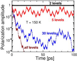
Figure 1: Amplitude of the linear optical polarization of the ground exciton state at $T=150$ K, taking into account two, five, thirty, and all exciton levels in a CdSe QD (set A).

The amplitude of the time-dependent linear polarization after impulsive excitation in a CdSe QD at $T=150$ K is shown in Fig. 1 for set (A). In this case, due to the full charge neutrality of the electron-hole pair, $M_{11}({\bf q})=0$ holds, and the linear term $V_{L}$ vanishes. Thus we concentrate at the moment on the quadratic term $V_{Q}$, Eq. (3), which is in fact the only source of dephasing. For two excitonic levels [i.e., only one excited state $n=2$ contributes to Eq. (4), and the matrix $A_{nm}$, Eq. (8), reduces to a scalar] the polarization has only tiny oscillations close to unity. For five levels, it decays and then revives almost to unity after 20 ps. For 30 levels, the amplitude decays already dramatically and then oscillates irregularly around a small value. Such a behavior has been already discussed before and called quasi-dephasing Stauber06 ; Jacak03a . Finally, if we take into account all excitonic states, the polarization decays strictly: At 100 ps its amplitude drops to $10^{-30}$ (but is shown in Fig. 1 only up to $10^{-8}$). In practice, of course, we truncate the infinite matrix $A_{nm}$ and check that a larger matrix produces no changes within the time interval considered.

To understand better why the optical polarization becomes decaying when more and more exciton (electron-hole pair) states are taken into account, we calculate the linear absorption spectrum, i.e. the real part of the Fourier transform of $P(t)$. It is hopeless, however, to find the Fourier transform numerically if the function does not decay at all or decays very weakly. That is why we use here a different method: We diagonalize exactly the excited state Hamiltonian $H_{1}$ which is related to the full one, Eq. (1), as $H=H_{0}|0\rangle\langle 0|+H_{1}|1\rangle\langle 1|$. Such a diagonalization is very easy if $V_{L}=0$. In case of two levels $H_{1}$ becomes

$$H^{\rm 2lev}_{1}=\Omega B^{\dagger}B+\tilde{E_{1}}+\omega_{0}\sum_{\mu}b^{\dagger}_{\mu}b_{\mu}\,,$$ (10)

where

$$\Omega = \sqrt{\omega_{0}^{2}-2\omega_{0}\sum_{\bf q}F_{2}(-{\bf q})F_{2}({\bf q})},$$ (11)

$$B = \sum_{\bf q}F_{2}({\bf q})(\xi_{+}a_{\bf q}+\xi_{-}a^{\dagger}_{-\bf q})$$ (12)

are, respectively, the new phonon frequency and annihilation operator, $\xi_{\pm}=(\Omega\pm\omega_{0})/2\sqrt{\omega_{0}\Omega\sum_{\bf q}|F_{2}({\bf q})|^{2}}$, and $\tilde{E_{1}}$ is the polaron shifted transition energy.

Note that out of a continuum of degenerate LO modes only a single phonon mode couples to the QD and produces a new, bound mode Dean70 $B$ with frequency $\Omega$, while all the other modes $b_{\mu}$, which show up in the last term of Eq. (10), are decoupled. They are simply some orthogonal linear combinations of the former phonon modes $a_{\bf q}$ and have the same old frequency $\omega_{0}$. The linear polarization $P(t)=\theta(t)\langle e^{iH_{0}t}e^{-iH_{1}t}\rangle$, calculated in the same way as in Ref. Stauber06 , then takes the form:

$$P^{\rm 2lev}(t)=\theta(t)\sum_{\mathbf{n,m}=0}^{\infty}\alpha_{\mathbf{nm}}\exp\{i(\mathbf{n}\omega_{0}-\mathbf{m}\Omega)t\},$$ (13)

where $\alpha_{\mathbf{nm}}=(1-e^{-\beta\omega_{0}})e^{-\beta\mathbf{n}\omega_{0}}|\mathbf{\langle n|m)}|^{2}$, and $\mathbf{\langle n|m)}$ are the projections of new phonon states $\mathbf{|m)}$ into old ones $\mathbf{|n\rangle}$ (to be distinguished from exciton states $|n\rangle$), which are calculated recursively.

Generalization to ${\cal N}$ excitonic levels is straightforward: $H_{1}$ is now diagonalized to ${\cal N}-1$ new phonon modes:

$$\Omega_{\nu}=\sqrt{\omega_{0}^{2}-2\omega_{0}\Lambda_{\nu}}$$ (14)

with $\Lambda_{\nu}$ being the eigenvalues of the $({\cal N}-1)$-dimensional matrix Eq. (8). In accordance with Eqs. (5) and (7), the full linear polarization can be written as a product

$$P(t)=\prod_{\nu}P_{\nu}(t)$$ (15)

of functions $P_{\nu}(t)$ due to each individual phonon mode given by the same Eq. (13), where $\Omega$ and $\alpha_{\mathbf{nm}}$ are replaced, respectively, by $\Omega_{\nu}$ and $\alpha^{\nu}_{\mathbf{nm}}$.

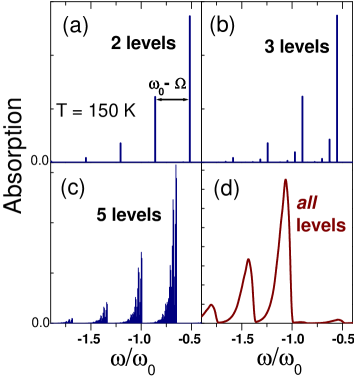
Figure 2: Evolution of the fine structure in the absorption spectrum of a QD by accounting for more and more excitonic levels [linear scale, set (A), $E_{1}$ is taken as zero of energy].

For two levels, the absorption spectrum, already discussed in Ref. Muljarov06 , represents a set of discrete lines. There are two-phonon satellites around the zero-phonon line (the standard one-phonon satellites are absent here as $V_{L}=0$), but more important is the fine structure shown in Fig. 2 (a). This fine structure is due to the difference between the old and the new phonon frequency $\omega_{0}-\Omega$ and manifests itself in the time domain as rapid oscillations with the period of 0.5 ps (Fig. 1). Including the third excitonic level brings in an additional frequency and more lines in the spectrum, Fig. 2 (b). With five levels (and four new phonon frequencies), there is already a plenty of closely lying delta lines, Fig. 2 (c). Finally, if we include all exciton levels, these lines merge and produce a continuous broadening, Fig. 2 (d). In the time domain, the polarization represents a superposition of individual oscillations [see Eqs. (15) and (13)] which interfere destructively due to incommensurability of their frequencies and thus lead to dephasing.

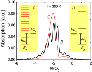
Figure 3: Absorption spectrum of a CdSe QD at $T=300$ K, calculated for two different types of the bare-exciton level structure [sets (B) and (C), see text]. Bound phonon frequencies $\Omega_{\nu}$ and levels $E_{n}$ of exciton excited (ground) states are shown in the insets by thin (thick) horizontal lines.

In contrast to the present model of a QD with discrete exciton levels only, in realistic QD systems there is also a wetting-layer continuum. This continuum could seem to be a more probable candidate for producing the spectral broadening Seebeck05 . It turns out, however, that in typical QDs, there are usually enough discrete exciton levels to provide an appreciable polarization decay. In fact, taking into account 30 levels is already sufficient to have the dephasing time very close to the exact one (i.e., with all levels, see Fig. 1), but at the same time it requires the heterostructure potential band offset to be less than 1.0 eV for the electron and 0.5 eV for the hole footnote . We account for all discrete levels in the harmonic potentials just for consistency, in order to show that a complete decay of the polarization is indeed achieved.

The full absorption spectrum of a CdSe QD is shown in Fig. 3. As we have in sets (B) and (C) different Gauss lengths, $l_{e}\neq l_{h}$, the linear coupling $V_{L}$ contributes too, which gives surprisingly only a slight modification in the spectrum. For set (B) all the excited levels are well above $\hbar\omega_{0}$. All the bound-phonon frequencies $\Omega_{\nu}$ are condensed just below $\omega_{0}$, except one which is well separated and is in fact responsible for the spectral fine structure. This fine structure is absent if we take a larger dot with closer levels (Fig. 3, red curve and inset C). Here, one excited level is found below $\hbar\omega_{0}$, and even two bound phonons are well resolved and wash out the fine

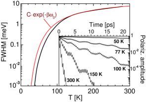
Figure 4: Spectral linewidth of the ground exciton state in a CdSe QD, set (B), as a function of temperature (solid curve) and the exponential fit with $C=20$ meV (dashed curve). Inset: Polarization amplitude at different temperatures.

structure. Thus, changes in the exciton level structure modify the spectrum but obviously do not affect our principal conclusion on the finite spectral width, and even do not alter much the linewidth itself.

Since the decay is not strictly exponential (see the inset in Fig. 4), we have extracted the linewidth directly from the absorption and plotted in Fig. 4 the full width at half maximum (FWHM) as a function of temperature. At high temperatures, the FWHM varies from few to ten meV and can be well approximated by an exponential law with $\hbar\omega_{0}$ being the activation energy. Below 50 K the linewidth is practically unaffected by LO phonons, and the dephasing in QDs is determined by some other mechanisms like coupling to acoustic phonons Muljarov04 , phonon anharmonicity Machnikowski06 , and radiative decay.

In conclusion, we have calculated the time-dependent optical polarization and the absorption spectrum of a quantum dot using the exactly solvable model of excitons quadratically coupled to LO phonons. We have extended this model to an arbitrary number of excitonic states in a quantum dot and (using its exact solution) demonstrated that taking into account infinitely many states results in an LO phonon-induced exciton dephasing and spectral broadening.

Financial support by DFG Sonderforschungsbereich 296 is gratefully acknowledged. E. A. M. acknowledges partial support by Russian Foundation for Basic Research and Russian Academy of Sciences.

References

- (1) U. Bockelmann and G. Bastard, Phys. Rev. B 42, 8947 (1990).
- (2) P. Borri et al., Phys. Rev. Lett. 87, 157401 (2001).
- (3) U. Bockelmann, Phys. Rev. B 48, 17637 (1993).
- (4) E. A. Muljarov and R. Zimmermann, Phys. Rev. Lett. 93, 237401 (2004).
- (5) S. Hameau et al., Phys. Rev. Lett. 83, 4152 (1999).
- (6) T. Stauber, R. Zimmermann, and H. Castella, Phys. Rev. B 62, 7336 (2000).
- (7) O. Verzelen, R. Ferreira, and G. Bastard, Phys. Rev. Lett. 88, 146803 (2002).
- (8) L. Jacak, J. Krasnyj, D. Jacak, and P. Machnikowski, Phys. Rev. B 67, 035303 (2003).
- (9) T. Stauber and R. Zimmermann, Phys. Rev. B 73, 115303 (2006).
- (10) T. Inoshita and H. Sakaki, Phys. Rev. B 56, R4355 (1997).
- (11) K. Král and Z. Khás, Phys. Rev. B 57, R2061 (1998).
- (12) A. V. Uskov et al., Phys. Rev. Lett. 85, 1516 (2000).
- (13) E. A. Muljarov and R. Zimmermann, Phys. Rev. Lett. 96, 019703 (2006).
- (14) P. J. Dean, D. D. Manchon Jr., and J. J. Hopfield, Phys. Rev. Lett. 25, 1027 (1970).
- (15) L. Jacak, P. Machnikowski, J. Krasnyj, and P. Zoller, Eur. Phys. J. D 22, 319 (2003).
- (16) J. Seebeck, T. R. Nielsen, P. Gartner, and F. Jahnke, Phys. Rev. B 71, 125327 (2005).
- (17) Electron (hole) energy levels are given by , where meV and meV Stauber06 in case (B); 30 levels are produced by taking and .
- (18) P. Machnikowski, Phys. Rev. Lett. 96, 140405 (2006).