Frequency-dependent current correlation functions from scattering theory

Abstract

We present a general formalism based on scattering theory to calculate quantum correlation functions involving several time-dependent current operators. A key ingredient is the causality of the scattering matrix, which allows one to deal with arbitrary correlation functions. Our formalism might be useful in view of recent developments in full counting statistics of charge transfer, where detecting schemes have been proposed for measurement of frequency dependent spectra of higher moments. Some of these schemes are different from the well-known fictitious spin-detector and therefore generally involve calculation of non-Keldysh-contour-ordered correlation functions. As an illustration of our method we consider various third order correlation functions of current, including the usual third cumulant of current statistics. We investigate the frequency dependence of these correlation functions explicitly in the case of energy-independent scattering. The results can easily be generalized to the calculation of arbitrary $n$-th order correlation functions, or to include the effect of interactions.

I Introduction

Dynamical noise properties of mesoscopic systems have been studied for more than a decade, both theoretically and experimentally blanter00 . By now it is well understood that noise measurements can reveal information on the system that is not contained in its DC conductance. So far, most experiments concentrated on measurement of zero-frequency noise. However, several proposals have considered the possibility of detecting finite-frequency noise, for instance through emission and absorption measurements using quantum few level systems like quantum dots aguado00 or small Josephson junctions schoelkopf03 as noise detectors. Successful experiments of this type have been reported recently deblock0306 ; astafiev04 . Finite frequency noise is interesting, first of all as one expects the noise to probe the intrinsic dynamics of the conductor and hence the noise spectral function should be sensitive to the dwell time $\tau_{D}$ of the carriers. Second, at finite frequency, current is no longer spatially homogeneous, and charge piles up in the conductor. Coulomb interaction screens this pile-up of charge, at a characteristic charge relaxation frequency $1/\tau$ which may well be different from $1/\tau_{D}$. These issues have been studied theoretically for diffusive contacts in Refs. naveh97 ; nagaev98 . Recent calculations of current noise in chaotic cavities nagaev04 ; hekking05 that take both the energy-dependence of scattering and Coulomb interactions into account show that the frequency-dependent noise spectrum is determined solely by the time $\tau$, as long as quantum corrections like weak-localization can be ignored. In view of recent interest in the theory of the full counting statistics (FCS) of charge transfer nazarov03 , attention shifted from the conventional noise to the study of the properties of the higher moments. Recent measurements have probed the zero-frequency third cumulant reulet03 ; bomze05 ; gustavsson:076605 . As far as the frequency dependence of the higher cumulants is concerned, the situation changes drastically as compared to conventional noise spectra. Calculations of the frequency-dependent third cumulant for a chaotic cavity nagaev04 and for a diffusive conductor pilgram04 show marked differences from the conventional noise: it is not only determined by the charge-relaxation time $\tau$ but also shows a low-frequency dispersion that is determined by the dwell time $\tau_{D}$.

A properly designed experiment, capable of measuring the frequency-dependent third cumulant, would thus enable one to determine the two relevant time scales separately in a mesoscopic conductor. The question as to how to design such an experiment brings us to one of the key problems of this field: what is an adequate detector to measure frequency-dependent noise spectra, and which noise spectral function is it actually measuring? Most of the applications of FCS discussed so far concentrate on the use of a fictitious spin detector, introduced by Levitov and coworkers levitov94 ; levitov96 . This detector measures Keldysh contour-ordered correlation functions of current. Powerful theoretical tools have been developed to calculate these correlation functions; therefore this detector is amenable to straightforward analysis. However, the spin detector might not be the most suitable one for detecting finite frequency noise. Detectors that interact with the noise source through emission and absorption, like the abovementioned quantum detectors might be more suitable for this task. The measured spectra are then not directly related to Keldysh-ordered correlation functions, and different methods are required to determine these spectra theoretically.

In this paper we develop a method capable of handling arbitrarily ordered correlation functions. The formalism we adopt is based on scattering theory buttiker92 , pioneered in lesovik89 ; yurke90 ; buttiker90 . It is the natural approach to discuss transport and noise in mesoscopic devices. The operator for electric current $\hat{I}$ is written as the difference between the current carried by incident particles $\hat{I}_{\text{in}}$ and the current carried by scattered particles $\hat{I}_{\text{out}}$: $\hat{I}=\hat{I}_{\text{in}}-\hat{I}_{\text{out}}$. The central quantity of the scattering approach is the energy-dependent scattering matrix. It must satisfy the causality condition in real-time representation, which has immediate consequences for the commutation relations between the operators $\hat{I}_{\text{in}}$ and $\hat{I}_{\text{out}}$ at different times beenakker01 . As a result, any (anti) time-ordered product of current operators can be conveniently rewritten as products of currents $\hat{I}_{\text{in}}$ and $\hat{I}_{\text{out}}$ with all in-currents ordered to the right (left) of the out-currents. Denoting (anti) time-ordering by $T$ ($\tilde{T}$) this implies $T[\hat{I}_{\text{in}}(t_{1})\hat{I}_{\text{out}}(t_{2})]=\hat{I}_{\text{out}}(t_{2})\hat{I}_{\text{in}}(t_{1})$ and $\tilde{T}[\hat{I}_{\text{in}}(t_{1})\hat{I}_{\text{out}}(t_{2})]=\hat{I}_{\text{in}}(t_{1})\hat{I}_{\text{out}}(t_{2})$ independent of the ordering of $t_{1}$ and $t_{2}$. This way, the cumbersome time-ordering can be avoided and the remaining in-out -ordered products can be readily calculated using the scattering theory.

We apply the in-out -ordering method to the well-studied case of the third cumulant of charge transfer in a mesoscopic conductor. We treat energy-independent scattering, and present the time-dependent cumulant in the cases of a tunnel barrier (a quantum point contact), a diffusive wire, and a chaotic cavity. First of all, this enables a direct check on the validity of our method. Second, we believe that the zero frequency limit of the calculation provides a demonstration of the validity of the result for the third cumulant of a tunnel barrier presented in levitov04 . This result had given rise to some discussion in the literature levitov92 ; levitov94 ; levitov96 and methods have been developed to settle the issue in a frequency-dependent context lesovik03 ; galaktionov03 . Thirdly, our calculation of the frequency-dependent third cumulant enables us to find the asymptotic time-dependence of the third cumulant of the charge transfer, both in the short and the long time limits.

The paper is organized as follows: we first summarize the scattering formalism in order to define the notation used later, and use the causality of the scattering matrix to derive important commutation relations between in- and out-current operators. They are used to establish operator transformation rules, such as $T[\hat{I}_{\text{in}}(t_{1})\hat{I}_{\text{out}}(t_{2})]=\hat{I}_{\text{out}}(t_{2})\hat{I}_{\text{in}}(t_{1})$, which allow one to resolve time-ordered products of currents in terms of in-out -ordered products. Their main application is to find multi-current correlation functions, and we explicitly present all three-current correlations, which are written in terms of three-current spectral functions of two frequency arguments. To keep the presentation transparent, we do not address here issues concerning the finite dwell time of carriers nor do we address interaction effects. We thus treat the case of energy-independent scattering where the various spectral functions can be evaluated using only the transmission probabilities of the scatterer, valid in the limit where the above-mentioned characteristic times $\tau_{D}$, $\tau$ vanish. It is important to note that, even though we neglect the energy dependence of the scattering matrix, we do respect its causality through the in-out -ordering properties. We finally discuss several different detection schemes, which all correspond to different three-current correlation functions and, most importantly, use the full-counting statistics approach to derive an expression to the time-dependent third cumulant of transmitted charge distribution.

II Scattering formalism and causality

II.1 Scattering theory

The starting point for our analysis is scattering theory, as developed by Büttiker buttiker92 . In this formalism, the current operator of non-interacting electrons is given by

$$\begin{split}\hat{I}_{\alpha}(t)&=\frac{e}{h}\sum_{n}\int dEdE^{\prime}e^{i(E-E^{\prime})t/\hbar}[\hat{a}^{\dagger}_{\alpha n}(E)\hat{a}_{\alpha n}(E^{\prime})-\hat{b}^{\dagger}_{\alpha n}(E)\hat{b}_{\alpha n}(E^{\prime})].\end{split}$$ (1)

The operators $\hat{a}^{\dagger}_{\alpha n}(E)$ and $\hat{a}_{\alpha n}(E)$ create and annihilate electrons with total energy $E$ in the transverse channel $n$ in lead $\alpha$, incident upon the scatterer. Similarly, the creation $\hat{b}^{\dagger}_{\alpha n}(E)$ and annihilation $\hat{b}_{\alpha n}(E)$ operators refer to electrons in the outgoing states. For the two-terminal set-up depicted in Fig. 1, $\alpha$ takes values $L$ and $R$ for the left and right leads respectively. The results to be presented below can be easily generalized to any multi-terminal case.

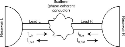
Figure 1: Two-terminal scattering problem. Both reservoirs are assumed to be in thermal equilibrium, characterized by a common temperature $T$ and potentials such that $V_{R}-V_{L}=V$.

The creation and annihilation operators obey the anticommutation relations, for instance,

$$\begin{split}\hat{a}^{\dagger}_{\alpha n}(E)\hat{a}_{\alpha n^{\prime}}(E^{\prime})+\hat{a}_{\alpha n^{\prime}}(E^{\prime})\hat{a}^{\dagger}_{\alpha n}(E)&=\delta_{nn^{\prime}}\delta(E-E^{\prime})\\ \hat{a}^{\dagger}_{\alpha n}(E)\hat{a}^{\dagger}_{\alpha n^{\prime}}(E^{\prime})+\hat{a}^{\dagger}_{\alpha n^{\prime}}(E^{\prime})\hat{a}^{\dagger}_{\alpha n}(E)&=0\\ \hat{a}_{\alpha n}(E)\hat{a}_{\alpha n^{\prime}}(E^{\prime})+\hat{a}_{\alpha n^{\prime}}(E^{\prime})\hat{a}_{\alpha n}(E)&=0.\end{split}$$ (2)

Similar anticommutation relations hold naturally also for operators referring to the outgoing states.

The operators $\hat{a}$ and $\hat{b}$ are related by the scattering matrix $s$,

$$\hat{b}_{\alpha n}(E)=\sum_{\beta,m}s_{\alpha\beta;nm}(E)\hat{a}_{\beta m}(E)$$ (3)

and the creation operators $\hat{a}^{\dagger}$ and $\hat{b}^{\dagger}$ are correspondingly related by the hermitian conjugated matrix, $s^{\dagger}_{\alpha\beta;nm}(E)=s^{*}_{\alpha\beta;mn}(E)$.

The matrix $s$ is quite generally unitary and it has dimensions $(N_{L}+N_{R})\times(N_{L}+N_{R})$. Its size and the matrix elements depend on the total energy $E$. It has the block structure

$$s=\left(\begin{array}[]{cc}r&t^{\prime}\\ t&r^{\prime}\end{array}\right).$$ (4)

Electron reflection back to the left and right reservoirs is described by the square diagonal blocks $r$ (size $N_{L}\times N_{L}$) and $r^{\prime}$ (size $N_{R}\times N_{R}$), respectively, while the off-diagonal, rectangular blocks $t$ (size $N_{R}\times N_{L}$) and $t^{\prime}$ (size $N_{L}\times N_{R}$) determine, in turn, the electron transmission through the sample.

In order to directly benefit from consequences of causality, we present the current operator as the difference between two directed currents, carried by incoming states and outgoing states, respectively beenakker01 . Specializing to the left lead, we thus write

$$\hat{I}_{L}(t)=\hat{I}_{L,\text{in}}(t)-\hat{I}_{L,\text{out}}(t),$$ (5)

where

$$\hat{I}_{L,\text{in}}(t)=\frac{e}{h}\sum_{n}\int dEdE^{\prime}e^{i(E-E^{\prime})t/\hbar}\hat{a}^{\dagger}_{Ln}(E)\hat{a}_{Ln}(E^{\prime}),$$ (6)

and

$$\hat{I}_{L,\text{out}}(t)=\frac{e}{h}\sum_{n}\int dEdE^{\prime}e^{i(E-E^{\prime})t/\hbar}\hat{b}^{\dagger}_{Ln}(E)\hat{b}_{Ln}(E^{\prime}).$$ (7)

Now, using Eq. (3) as well as its hermitian conjugated version, $\hat{I}_{L,\text{out}}(t)$ can also be written as

$$\begin{split}\hat{I}_{L,\text{out}}(t)=\frac{e}{h}\sum_{\alpha,\beta}\sum_{mnk}\int dEdE^{\prime}e^{i(E-E^{\prime})t/\hbar}\hat{a}^{\dagger}_{\alpha m}(E)s^{\dagger}_{L\alpha;mk}(E)s_{L\beta;kn}(E^{\prime})\hat{a}_{\beta n}(E^{\prime}),\end{split}$$ (8)

where indices $\alpha$ and $\beta$ may take values $L$ or $R$. This result makes the dependence of the current operator $\hat{I}_{\mathrm{out}}$ on the energy-dependent scattering matrix $s(E)$ explicit. As we will detail below, the commutation properties of directed current operators at different times are completely determined by the analytical properties of $s(E)$.

II.2 Causality

In real time, the scattering matrix connects operators of an incoming state with those of an outgoing state by the convolution relation

$$\hat{b}_{\alpha n}(t)=\sum_{\beta,m}\int_{-\infty}^{\infty}s_{\alpha\beta;nm}(t-\tau)\hat{a}_{\beta m}(\tau){\rm d}\tau.$$ (9)

By causality, the scattering matrix must vanish for negative arguments since otherwise an incident current at $t_{1}$ would cause an outgoing current at $t_{2}<t_{1}$. This is equivalent to requiring that the Fourier transform of the scattering matrix, $s_{\alpha\beta;nm}(\omega)$ be analytic in the entire upper half plane, since then

$$s_{\alpha\beta;nm}(\omega)=\lim_{\eta\rightarrow 0^{+}}\int_{-\infty}^{\infty}\frac{d\omega^{\prime}}{2\pi i}\frac{s_{\alpha\beta;nm}(\omega^{\prime})}{(\omega^{\prime}-\omega)-i\eta},$$ (10)

which can be substituted into the inverse Fourier transform of the scattering matrix in order to obtain

$$\begin{split}s_{\alpha\beta;nm}(t)&=\int_{-\infty}^{\infty}\frac{d\omega^{\prime}}{2\pi}s_{\alpha\beta;nm}(\omega^{\prime})\int_{-\infty}^{\infty}\frac{d\omega}{2\pi i}e^{-i\omega t}\frac{1}{(\omega^{\prime}-\omega)-i\eta}=\theta(t)s_{\alpha\beta;nm}(t).\end{split}$$ (11)

Hence the analytical structure of $s(\omega)$ as a function of $\omega$ (analyticity in the entire upper half plane) implies causality shepard91 ; buttiker93 , i.e., $s(t-t^{\prime})=0$ if $t<t^{\prime}$. Similarly, the hermitian conjugated scattering matrix, $s^{\dagger}_{\alpha\beta;nm}(\omega)$, must be analytic in the entire lower half plane.

II.3 Commutation relations

We will use the analytical structure of the scattering matrix established in the previous subsection, Eq. (11), to obtain the commutation relations for directed current operators $\hat{I}_{\mathrm{in}}$ and $\hat{I}_{\mathrm{out}}$ at different times beenakker01 . Consider the commutation relation of $\hat{I}_{L,\text{in}}(t_{1})$ and $\hat{I}_{L,\text{out}}(t_{2})$. Starting from

$$\begin{split}&[\hat{I}_{L,\text{in}}(t_{1}),\hat{I}_{L,\text{out}}(t_{2})]\\ &=\left(\frac{e}{h}\right)^{2}\sum\limits_{n_{1},n_{2}}\int dE_{1}dE_{2}dE_{3}dE_{4}e^{i(E_{1}-E_{2})t_{1}/\hbar}e^{i(E_{3}-E_{4})t_{2}/\hbar}[\hat{a}^{\dagger}_{Ln_{1}}(E_{1})\hat{a}_{Ln_{1}}(E_{2}),\hat{b}^{\dagger}_{Ln_{2}}(E_{3})\hat{b}_{Ln_{2}}(E_{4})],\end{split}$$ (12)

and applying the commutation relations as given in (2) we find that

$$\begin{split}&[\hat{I}_{L,\text{in}}(t_{1}),\hat{I}_{L,\text{out}}(t_{2})]\\ &=\left(\frac{e}{h}\right)^{2}\sum_{n_{1},n_{2}}\int dE_{1}dE_{2}dE_{3}\big{[}e^{i(E_{1}-E_{3})t_{1}/\hbar}e^{i(E_{3}-E_{2})t_{2}/\hbar}\hat{a}^{\dagger}_{Ln_{1}}(E_{1})s^{\dagger}_{LL;n_{1}n_{2}}(E_{3})\hat{b}_{Ln_{2}}(E_{2})\\ &\qquad\qquad\qquad\qquad\qquad\qquad\qquad-e^{i(E_{3}-E_{2})t_{1}/\hbar}e^{i(E_{1}-E_{3})t_{2}/\hbar}\hat{b}^{\dagger}_{Ln_{2}}(E_{1})s_{LL;n_{2}n_{1}}(E_{3})\hat{a}_{Ln_{1}}(E_{2})\big{]}.\end{split}$$ (13)

Integrating over all energies we obtain

$$\begin{split}[\hat{I}_{L,\text{in}}(t_{1}),\hat{I}_{L,\text{out}}(t_{2})]=he^{2}\sum_{n_{1},n_{2}}\hat{a}^{\dagger}_{Ln_{1}}(t_{1})s^{\dagger}_{LL;n_{1}n_{2}}(t_{2}-t_{1})\hat{b}_{Ln_{2}}(t_{2})-\hat{b}^{\dagger}_{Ln_{2}}(t_{2})s_{LL;n_{2}n_{1}}(t_{2}-t_{1})\hat{a}_{Ln_{1}}(t_{1}).\end{split}$$ (14)

According to Eq. (11) the commutator (14) vanishes identically if $t_{1}$ is a later instant of time than $t_{2}$ beenakker01 . We thus conclude that

$$[\hat{I}_{L,\text{in}}(t_{1}),\hat{I}_{L,\text{out}}(t_{2})]\propto\theta(t_{2}-t_{1}).$$ (15)

We obtain the commutation relations for $\hat{I}_{L,\text{in}}(t_{1})$ and $\hat{I}_{L,\text{in}}(t_{2})$, and for $\hat{I}_{L,\text{out}}(t_{1})$ and $\hat{I}_{L,\text{out}}(t_{2})$ using the same procedure: both these vanish identically,

$$[\hat{I}_{L,\text{in}}(t_{1}),\hat{I}_{L,\text{in}}(t_{2})]=0$$ (16)

and

$$[\hat{I}_{L,\text{out}}(t_{1}),\hat{I}_{L,\text{out}}(t_{2})]=0.$$ (17)

These commutation relations have important consequences for the calculation of time-ordered correlation functions involving the operators $\hat{I}_{\text{in}}(t)$ and $\hat{I}_{\text{out}}(t)$, as we will now show.

II.4 Time-ordered correlation functions

We denote the time-ordering of operators by $T[A(t_{1})B(t_{2})C(t_{3})\dots]$, where the operators appear in descending order of times, and the anti-time-ordering by $\tilde{T}[A(t_{1})B(t_{2})C(t_{3})\dots]$, with the opposite order of times. Specifically, making use of (15), (16), and (17), we find the following operator identities:

$$\begin{split}T[\hat{I}_{\text{in}}(t_{1})\hat{I}_{\text{in}}(t_{2})]&=\hat{I}_{\text{in}}(t_{1})\hat{I}_{\text{in}}(t_{2}),\\ T[\hat{I}_{\text{out}}(t_{1})\hat{I}_{\text{out}}(t_{2})]&=\hat{I}_{\text{out}}(t_{1})\hat{I}_{\text{out}}(t_{2}),\\ T[\hat{I}_{\text{in}}(t_{1})\hat{I}_{\text{out}}(t_{2})]&=\hat{I}_{\text{out}}(t_{2})\hat{I}_{\text{in}}(t_{1}),\\ T[\hat{I}_{\text{out}}(t_{1})\hat{I}_{\text{in}}(t_{2})]&=\hat{I}_{\text{out}}(t_{1})\hat{I}_{\text{in}}(t_{2}).\end{split}$$ (18)

One therefore concludes beenakker01 : time-ordering a product of directed current operators corresponds to an ordering in which all the out-currents $\hat{I}_{\mathrm{out}}$ are placed to the left of the in-currents $\hat{I}_{\mathrm{in}}$.

As an example, let us consider the two lowest time-ordered correlation functions. Using $\hat{I}(t)=\hat{I}_{\text{in}}(t)-\hat{I}_{\text{out}}(t)$, one obtains

$$\begin{split}&T[\hat{I}(t_{1})\hat{I}(t_{2})]=\hat{I}_{\text{in}}(t_{1})\hat{I}_{\text{in}}(t_{2})-\hat{I}_{\text{out}}(t_{2})\hat{I}_{\text{in}}(t_{1})-\hat{I}_{\text{out}}(t_{1})\hat{I}_{\text{in}}(t_{2})+\hat{I}_{\text{out}}(t_{1})\hat{I}_{\text{out}}(t_{2}),\end{split}$$ (19)

and

$$\begin{split}T[\hat{I}(t_{1})\hat{I}(t_{2})\hat{I}(t_{3})]&=\hat{I}_{\text{in}}(t_{1})\hat{I}_{\text{in}}(t_{2})\hat{I}_{\text{in}}(t_{3})-\hat{I}_{\text{out}}(t_{3})\hat{I}_{\text{in}}(t_{1})\hat{I}_{\text{in}}(t_{2})-\hat{I}_{\text{out}}(t_{2})\hat{I}_{\text{in}}(t_{1})\hat{I}_{\text{in}}(t_{3})\\ &\quad-\hat{I}_{\text{out}}(t_{1})\hat{I}_{\text{in}}(t_{2})\hat{I}_{\text{in}}(t_{3})+\hat{I}_{\text{out}}(t_{2})\hat{I}_{\text{out}}(t_{3})\hat{I}_{\text{in}}(t_{1})+\hat{I}_{\text{out}}(t_{1})\hat{I}_{\text{out}}(t_{3})\hat{I}_{\text{in}}(t_{2})\\ &\quad+\hat{I}_{\text{out}}(t_{1})\hat{I}_{\text{out}}(t_{2})\hat{I}_{\text{in}}(t_{3})-\hat{I}_{\text{out}}(t_{1})\hat{I}_{\text{out}}(t_{2})\hat{I}_{\text{out}}(t_{3}).\end{split}$$ (20)

For the ordered $n$-current correlation function, the number of terms containing $p$ out-currents and $n-p$ in-currents is just the binomial factor $n!/[p!(n-p)!]$. The sign of such a term is $(-1)^{p}$. The anti-time-ordering $\tilde{T}$ can be dealt with analogously, but here the in and out currents are ordered oppositely: all the out-currents stand to the right of the in-currents.

The important point here, and one of the central conclusions of Ref. beenakker01 , is that using in-out ordering one gets rid of the cumbersome limits of time integration, normally present in time-ordered expressions. This will enable us in the following to straightforwardly calculate Fourier transforms and hence directly obtain the frequency-dependent spectral functions of the relevant correlation functions. Moreover, the idea of ordering currents using the in-out formalism is quite natural in scattering theory.

III In-out three-current spectral functions

III.1 General results

We now turn to consider various three-current correlation functions of the form $\langle\delta\hat{I}_{L,x}(t_{1})\delta\hat{I}_{L,y}(t_{2})\delta\hat{I}_{L,z}(t_{3})\rangle$, where each of the $x$, $y$, and $z$ refers to the directed component of the current, either in or out, and $\delta\hat{I}=\hat{I}-\langle\hat{I}\rangle$. In the time-independent case, they can be expressed using the Fourier transform given by

$$\begin{split}&\langle\delta\hat{I}_{L,x}(t_{1})\delta\hat{I}_{L,y}(t_{2})\delta\hat{I}_{L,z}(t_{3})\rangle\equiv\int\frac{d\omega_{1}}{2\pi}e^{-i\omega_{1}(t_{1}-t_{2})}\int\frac{d\omega_{2}}{2\pi}e^{-i\omega_{2}(t_{2}-t_{3})}S_{xyz}(\omega_{1},\omega_{2}),\end{split}$$ (21)

where $S_{xyz}(\omega_{1},\omega_{2})$ are the corresponding three-current spectral functions. (Note that another convention is to take the transform with respect to $t_{1}-t_{2}$ and $t_{1}-t_{3}$, which leads to slightly redefined parameterization of the spectral functions.) Specializing to the case of equilibrium reservoirs, the spectral functions $S_{xyz}(\omega_{1},\omega_{2})$ are obtained by applying Wick’s theorem; we refer the reader to Appendix A for details. Specifically, we present results for the three-current spectral functions in the general case of an arbitrary energy-dependent scattering matrix in Table 2 of Appendix B, and for energy-independent scattering in Table 3 in the same Appendix. Here we just note that for the particular case of $S_{\text{in,in,in}}$, the energy integral contains Fermi functions of only one reservoir, and its value vanishes then identically. This is due to the fact that the in-in-in term does not contain the possibly energy-dependent scattering matrix. Spectral functions containing two in-currents also only depend on the Fermi function of the left reservoir, but the energy-dependence of the scattering matrix may render the integrals nonzero. Such terms, however, vanish in the case of energy-independent scattering so that four spectral functions out of the eight are identically zero. The four remaining spectra at zero temperature are depicted in Fig. 2 as functions of the two frequencies $\omega_{1}$ and $\omega_{2}$.

III.2 Limiting cases of in-out -ordered spectral functions

Although the true advantage of in-out ordering comes when dealing with general correlation functions, we demonstrate here that it also provides a straightforward way to obtain the spectral functions in some special cases which have been discussed in literature already earlier. In particular, we investigate here the case of energy-independent scattering in the limiting cases in terms of temperature, voltage, and the two frequencies.

As mentioned above, in the case of energy-independent scattering only four three-current spectral functions out of eight possible ones remain nonzero. At zero frequencies, $\omega_{1}=\omega_{2}=0$, only $S_{\text{out,in,out}}$ and $S_{\text{out,out,out}}$ are finite, with their values given by

$$\begin{split}S_{\text{out,in,out}}&=-eV\frac{e^{3}}{h}\sum_{n}T_{n}(1-T_{n})\equiv-\Gamma_{\text{A}}\\ S_{\text{out,out,out}}&=-eV\frac{e^{3}}{h}\sum_{n}T_{n}(1-T_{n})(1-2T_{n})\equiv-\Gamma_{\text{B}}\end{split}$$ (22)

where $\Gamma_{\text{A}}=e^{2}GVF_{2}$ and $\Gamma_{\text{B}}=e^{2}GVF_{3}$ are expressed in terms of the conductance, $G=\frac{e^{2}}{h}\sum_{n}T_{n}$, and the Fano factors of the second and third order, $F_{2}=\sum_{n}T_{n}(1-T_{n})/\sum_{n}T_{n}$ and $F_{3}=\sum_{n}T_{n}(1-T_{n})(1-2T_{n})/\sum_{n}T_{n}$. The transmission eigenvalues $\{T_{n}\}$ are the eigenvalues of the transmission matrix $t^{\dagger}t$. In the high-frequency limit, $|\omega_{1}|,|\omega_{2}|\gg eV/\hbar$, the non-vanishing terms are in turn $S_{\text{in,out,out}}$ and $S_{\text{out,out,in}}$, whose values equal $2\Gamma_{\text{A}}$ in the second and first octants, respectively, and $S_{\text{out,in,out}}=-2\Gamma_{\text{A}}$ in the first quadrant.

At finite temperatures such that $\hbar|\omega_{1}|,\hbar|\omega_{2}|\ll k_{B}T$, the spectral functions become independent of $\omega_{1}$ and $\omega_{2}$, and the non-vanishing ones are given by

$$\begin{split}S_{\text{in,out,out}}&=S_{\text{out,out,in}}=\frac{1}{3}\Gamma_{\text{A}}\\ S_{\text{out,in,out}}&=-\frac{2}{3}\Gamma_{\text{A}}.\end{split}$$ (23)

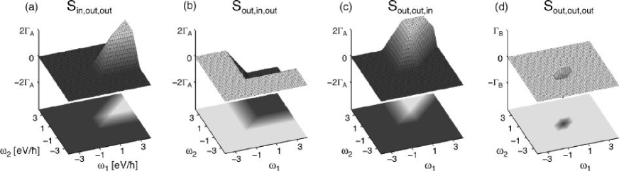
Figure 2: The non-vanishing contributions to zero-temperature three-current spectral functions $S_{\text{in,out,out}}$, $S_{\text{out,in,out}}$, $S_{\text{out,out,in}}$, and $S_{\text{out,out,out}}$ plotted against the frequencies $\omega_{1}$ and $\omega_{2}$. The first three of these have values between $0$ and $\pm 2\Gamma_{\text{A}}=\pm 2eV\frac{e^{3}}{h}\sum_{n}T_{n}(1-T_{n})$ while the last one has the extreme value of $-\Gamma_{\text{B}}=-eV\frac{e^{3}}{h}\sum_{n}T_{n}(1-T_{n})(1-2T_{n})$ at the origin and it vanishes at high frequencies, $|\omega_{1}|,|\omega_{2}|\gg eV/\hbar$.

IV Different physical detector schemes

An arbitrary three-current correlation function can always be decomposed into a sum of various in-out -ordered spectral functions of the type of Eq. (21), whose properties are, at least in principle, known. We will illustrate the usefulness of this decomposition scheme now for various examples of three-current correlation functions which have appeared in the literature. For simplicity we assume energy-independent scattering such that definite results can be obtained for three specific examples. We will first consider accumulated charge by a fictitious spin-detector levitov96 , which directly depends on the Keldysh-ordered correlation functions, and we use the in-out three-current spectral functions to evaluate time-dependent third cumulant of the charge distribution. We also compare this with current statistics derived from an unordered generating function and relate it to some of the results earlier appeared in literature. The second example is a classical detector which would correspond to the standard fully symmetrized three-current correlation function golubev05 , and finally we briefly discuss a partially time-ordered correlation function that appears when the time evolution of the density matrix of a multilevel quantum detector is considered, coupled to a non-gaussian noise source ojanen06 ; brosco06 .

IV.1 Third cumulant of FCS

The third cumulant of the full-counting statistics, i.e. the first correction term describing the deviation from the Gaussian distribution of the charge $q$ transported through the conductor during a time $t$, has been introduced in Refs. levitov94 and levitov96 , and it is given by

$$\begin{split}\langle\langle q^{3}\rangle\rangle=\int\limits_{0}^{t}dt_{1}\int\limits_{0}^{t}dt_{2}\int\limits_{0}^{t}dt_{3}S_{\text{K}}^{(3)}(t_{1},t_{2},t_{3}),\end{split}$$ (24)

where the Keldysh-contour ordered correlation function is given by

$$\begin{split}S_{\text{K}}^{(3)}(t_{1},t_{2},t_{3})&=\frac{1}{8}\langle\tilde{T}[\hat{I}_{L}(t_{1})\hat{I}_{L}(t_{2})\hat{I}_{L}(t_{3})]+T[\hat{I}_{L}(t_{1})\hat{I}_{L}(t_{2})\hat{I}_{L}(t_{3})]+3\tilde{T}[\hat{I}_{L}(t_{1})\hat{I}_{L}(t_{2})]\hat{I}_{L}(t_{3})+3\hat{I}_{L}(t_{1})T[\hat{I}_{L}(t_{2})\hat{I}_{L}(t_{3})]\rangle\\ &\quad-3\langle\hat{I}_{L}(t_{1})\rangle\langle\hat{I}_{L}(t_{2})\hat{I}_{L}(t_{3})\rangle+2\langle\hat{I}_{L}(t_{1})\rangle\langle\hat{I}_{L}(t_{2})\rangle\langle\hat{I}_{L}(t_{3})\rangle.\end{split}$$ (25)

Using the operator relations given by Eqs. (19) and (20), together with their anti-time-ordered counterparts, and regrouping the current operators into deviation operators $\delta\hat{I}_{\text{in,out}}(t)\equiv\hat{I}_{\text{in,out}}(t)-\langle\hat{I}_{\text{in,out}}(t)\rangle$, enables one to express this particular correlation function as

$$\begin{split}S_{\text{K}}^{(3)}(t_{1},t_{2},t_{3})&=\langle\delta\hat{I}_{L,\text{in}}(t_{1})\delta\hat{I}_{L,\text{in}}(t_{2})\delta\hat{I}_{L,\text{in}}(t_{3})-\frac{3}{4}\delta\hat{I}_{L,\text{in}}(t_{1})\delta\hat{I}_{L,\text{in}}(t_{2})\delta\hat{I}_{L,\text{out}}(t_{3})-\frac{3}{2}\delta\hat{I}_{L,\text{in}}(t_{1})\delta\hat{I}_{L,\text{out}}(t_{2})\delta\hat{I}_{L,\text{in}}(t_{3})\\ &\quad-\frac{3}{4}\delta\hat{I}_{L,\text{out}}(t_{1})\delta\hat{I}_{L,\text{in}}(t_{2})\delta\hat{I}_{L,\text{in}}(t_{3})+\frac{3}{2}\delta\hat{I}_{L,\text{in}}(t_{1})\delta\hat{I}_{L,\text{out}}(t_{2})\delta\hat{I}_{L,\text{out}}(t_{3})+\frac{3}{2}\delta\hat{I}_{L,\text{out}}(t_{1})\delta\hat{I}_{L,\text{out}}(t_{2})\delta\hat{I}_{L,\text{in}}(t_{3})\\ &\quad-\delta\hat{I}_{L,\text{out}}(t_{1})\delta\hat{I}_{L,\text{out}}(t_{2})\delta\hat{I}_{L,\text{out}}(t_{3})\rangle.\end{split}$$ (26)

Each term here can now be expressed in terms of the Fourier transform of the spectral function, Eq. (21), and the time integrals of Eq. (24) may be carried out explicitly. This results in

$$\begin{split}&\langle\langle q^{3}\rangle\rangle=2\int\frac{d\omega_{1}}{2\pi}\int\frac{d\omega_{2}}{2\pi}S_{\text{K}}^{(3)}(\omega_{1},\omega_{2})\frac{\sin(\omega_{2}t)-\sin(\omega_{1}t)+\sin[(\omega_{1}-\omega_{2})t]}{\omega_{1}\omega_{2}(\omega_{1}-\omega_{2})}\end{split}$$ (27)

where, for this particular ordering, we have

$$\begin{split}S_{\text{K}}^{(3)}(\omega_{1},\omega_{2})&=-\frac{3}{4}S_{\text{in,in,out}}(\omega_{1},\omega_{2})-\frac{3}{2}S_{\text{in,out,in}}(\omega_{1},\omega_{2})-\frac{3}{4}S_{\text{out,in,in}}(\omega_{1},\omega_{2})\\ &\quad+\frac{3}{2}S_{\text{in,out,out}}(\omega_{1},\omega_{2})+\frac{3}{2}S_{\text{out,out,in}}(\omega_{1},\omega_{2})-S_{\text{out,out,out}}(\omega_{1},\omega_{2}).\end{split}$$ (28)

This result is plotted in Fig. 3 (a) for energy-independent scattering at zero temperature. Note that the multiplier of each term in the sum above is obtained with the help of the binomial distribution. The particular ordering for current operators, like that in Eq. (25), determines the final weight of each $xyz$ spectral function.

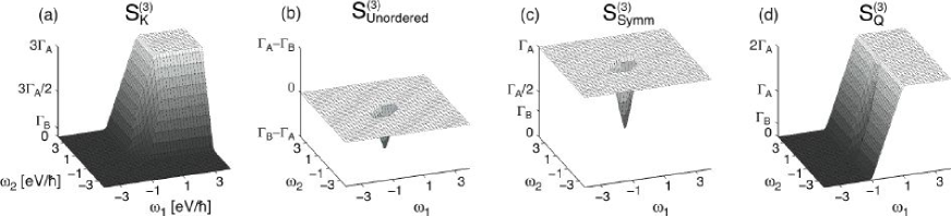
Figure 3: (a) Keldysh-ordered, (b) unordered, (c) symmetrized, and (d) non-symmetrized spectra at zero temperature. The saturated levels of the spectral functions are all proportional to $\Gamma_{\text{A}}$ except for the unordered spectrum, which saturates to zero. For the other spectra the level essentially depends on in which areas of the $(\omega_{1},\omega_{2})$–plane the spectrum has non-zero values. Both $S_{\text{in,out,out}}$ and $S_{\text{out,out,in}}$ vanish at zero frequency, and the spectral functions (a), (c), and (d) are then determined by $\Gamma_{\text{B}}=-S_{\text{out,out,out}}$, while the spectrum (b) is given by $\Gamma_{\text{B}}-\Gamma_{\text{A}}=S_{\text{out,in,out}}-S_{\text{out,out,out}}$, as indicated in the graph.

IV.1.1 Asymptotic values of the third cumulant

The third cumulant of FCS can be evaluated in the limits of both short and long times $t$. For short $t$ the cumulant is determined by the values of $S_{\text{K}}^{(3)}(\omega_{1},\omega_{2})$ at large frequencies where $S_{\text{out,out,out}}(\omega_{1},\omega_{2})$ is zero, and

$$\begin{split}S_{\text{K}}^{(3)}(\omega_{1},\omega_{2})=3eV\frac{e^{3}}{h}\sum_{n}T_{n}(1-T_{n})=3\Gamma_{\text{A}}\end{split}$$ (29)

nearly everywhere in the first quadrant of the $(\omega_{1},\omega_{2})$–plane and zero elsewhere. Therefore, the short-time value of the third cumulant is determined by the $S_{\text{in,out,out}}$ and $S_{\text{out,out,in}}$ spectral functions since only they have non-vanishing high-frequency values. We thus have

$$\begin{split}\langle\langle q^{3}\rangle\rangle&\approx 6teV\frac{e^{3}}{h}\sum_{n}T_{n}(1-T_{n})\int_{0}^{\infty}\frac{{\rm d}x_{1}}{2\pi}\int_{0}^{\infty}\frac{{\rm d}x_{2}}{2\pi}\frac{\sin x_{2}-\sin x_{1}+\sin(x_{1}-x_{2})}{x_{1}x_{2}(x_{1}-x_{2})}\\ &=teV\frac{e^{3}}{h}\sum_{n}T_{n}(1-T_{n})=\Gamma_{\text{A}}t.\end{split}$$ (30)

Value of the third cumulant for large $t$ is obtained in a similar manner. As long as $S_{\text{K}}^{(3)}(0,0)\neq 0$, the leading order is given by

$$\begin{split}&\langle\langle q^{3}\rangle\rangle=2\int\frac{d\omega_{1}}{2\pi}\int\frac{d\omega_{2}}{2\pi}S_{\text{K}}^{(3)}(\omega_{1},\omega_{2})\frac{\sin(\omega_{2}t)-\sin(\omega_{1}t)+\sin[(\omega_{1}-\omega_{2})t]}{\omega_{1}\omega_{2}(\omega_{1}-\omega_{2})}\approx tS_{\text{K}}^{(3)}(0,0).\end{split}$$

For $k_{B}T\ll eV$, only $S_{\text{out,out,out}}(0,0)=-\Gamma_{\text{B}}$ has a non-vanishing value in $S_{\text{K}}^{(3)}$ at $\omega_{1}=\omega_{2}=0$, and the linear growth at long times is then given by

$$\begin{split}\langle\langle q^{3}\rangle\rangle&=\Gamma_{\text{B}}t\end{split}$$ (31)

while, in the opposite regime, $k_{B}T\gg eV$, the directed three-current spectral functions become independent of the frequency arguments, and $S_{\text{K}}^{(3)}=eV\frac{e^{3}}{h}\sum_{n}T_{n}(1-T_{n})$; the long term cumulant is then given by

$$\langle\langle q^{3}\rangle\rangle=\Gamma_{\text{A}}t.$$ (32)

Since the Keldysh-ordered spectral function is independent of frequency as long as $|\omega_{1}|,|\omega_{2}|\ll k_{B}T/\hbar$, this result holds as long as $t\gg\hbar/k_{B}T$.

Both these results, Eqs. (31) and (32), are in agreement with those presented in Ref. levitov04 , and thus constitute a test of the correctness of our approach. Note in particular that we find $\langle\langle q^{3}\rangle\rangle/t=\Gamma_{\text{B}}\sim\sum_{n}T_{n}(1-T_{n})(1-2T_{n})$ for low temperature. This result has given rise to some discussion in the literature, since Ref. levitov92 obtained $\langle\langle q^{3}\rangle\rangle/t\sim\sum_{n}T_{n}^{2}(1-T_{n})$, different from Eq. (31). Several authors galaktionov03 ; lesovik03 subsequently developed methods to analyze frequency-dependent three-current correlation functions in order to assess the correctness of Eq. (31). In Ref. galaktionov03 an effective action approach together with an involved regularization procedure is used to establish Eq. (31). According to Ref. lesovik03 the frequency dependence of $S_{\rm K}$, and hence the result for $\langle\langle q^{3}\rangle\rangle$, depends on the actual position of the spin-detector with respect to the scatterer. Then, both results for $\langle\langle q^{3}\rangle\rangle$ cited above are found, depending on the position of the detector. A drawback is that the specific frequency-dependence of $S_{\rm K}$ postulated in Ref. lesovik03 generally does not conserve current. Let us address the issue here in the framework of the in-out-ordering technique. The $\sum_{n}T_{n}^{2}(1-T_{n})$ proportionality is obtained in Ref. levitov92 by considering a straightforward quantum analogue of the classical generating function, which leads to the cumulant

$$\begin{split}\langle\langle q^{3}\rangle\rangle=\left\langle\left(\int_{0}^{t}d\tau\delta\hat{I}(\tau)\right)^{3}\right\rangle=\int_{0}^{t}dt_{1}\int_{0}^{t}dt_{2}\int_{0}^{t}dt_{3}\left\langle\delta\hat{I}(t_{1})\delta\hat{I}(t_{2})\delta\hat{I}(t_{3})\right\rangle.\end{split}$$ (33)

Note that there is no specific time-ordering in this expression. Use of $\delta\hat{I}=\delta\hat{I}_{\text{in}}-\delta\hat{I}_{\text{out}}$ then leads to the entirely unordered correlation function

$$\begin{split}S_{\text{Unordered}}^{(3)}(t_{1},t_{2},t_{3})&=\langle\delta\hat{I}_{L,\text{in}}(t_{1})\delta\hat{I}_{L,\text{in}}(t_{2})\delta\hat{I}_{L,\text{in}}(t_{3})-\delta\hat{I}_{L,\text{in}}(t_{1})\delta\hat{I}_{L,\text{in}}(t_{2})\delta\hat{I}_{L,\text{out}}(t_{3})-\delta\hat{I}_{L,\text{in}}(t_{1})\delta\hat{I}_{L,\text{out}}(t_{2})\delta\hat{I}_{L,\text{in}}(t_{3})\\ &\quad-\delta\hat{I}_{L,\text{out}}(t_{1})\delta\hat{I}_{L,\text{in}}(t_{2})\delta\hat{I}_{L,\text{in}}(t_{3})+\delta\hat{I}_{L,\text{in}}(t_{1})\delta\hat{I}_{L,\text{out}}(t_{2})\delta\hat{I}_{L,\text{out}}(t_{3})+\delta\hat{I}_{L,\text{out}}(t_{1})\delta\hat{I}_{L,\text{out}}(t_{2})\delta\hat{I}_{L,\text{in}}(t_{3})\\ &\quad+\delta\hat{I}_{L,\text{out}}(t_{1})\delta\hat{I}_{L,\text{in}}(t_{2})\delta\hat{I}_{L,\text{out}}(t_{3})-\delta\hat{I}_{L,\text{out}}(t_{1})\delta\hat{I}_{L,\text{out}}(t_{2})\delta\hat{I}_{L,\text{out}}(t_{3})\rangle.\end{split}$$ (34)

The corresponding spectrum is given by

$$\begin{split}S_{\text{Unordered}}^{(3)}(\omega_{1},\omega_{2})&=-S_{\text{in,in,out}}(\omega_{1},\omega_{2})-S_{\text{in,out,in}}(\omega_{1},\omega_{2})-S_{\text{out,in,in}}(\omega_{1},\omega_{2})\\ &\quad+S_{\text{in,out,out}}(\omega_{1},\omega_{2})+S_{\text{out,in,out}}(\omega_{1},\omega_{2})+S_{\text{out,out,in}}(\omega_{1},\omega_{2})-S_{\text{out,out,out}}(\omega_{1},\omega_{2});\end{split}$$ (35)

it is plotted in Fig. 3 (b) for zero temperature. Here two terms on the right hand side of (35) contribute at zero frequency, namely $S_{\text{out,in,out}}$ and $S_{\text{out,out,out}}$. For the unordered three current correlator, we thus find that the corresponding third cumulant is given asymptotically (for large $t$) by

$$\begin{split}\langle\langle q^{3}\rangle\rangle&\approx(\Gamma_{\text{B}}-\Gamma_{\text{A}})t=-t2eV\frac{e^{3}}{h}\sum_{n}T_{n}^{2}(1-T_{n}),\end{split}$$ (36)

as found in Ref. levitov92 . We therefore conclude that the difference between this result and Eq. (31) is entirely due to the different ordering properties of the two definitions of $\langle\langle q^{3}\rangle\rangle$, Eqs. (33) and (27).

IV.1.2 Time-dependent third cumulant in various cases

$$\begin{array}[]{lcccc}&\text{Tunnel junction,}&\text{Chaotic cavity}&\text{Diffusive wire}\\ &0\leq T\ll 1&P(T)=\frac{1}{\pi}\frac{1}{\sqrt{T(1-T)}}&P(T)=\frac{l}{2L}\frac{1}{T\sqrt{(1-T)}}\\ \hline\cr\frac{1}{N}\langle\sum_{n}T_{n}\rangle&T_{\text{ave}}&\frac{1}{2}&\frac{l}{L}\\ \frac{1}{N}\langle\sum_{n}T_{n}(1-T_{n})\rangle&T_{\text{ave}}&\frac{1}{8}&\frac{1}{3}\frac{l}{L}\\ \frac{1}{N}\langle\sum_{n}T_{n}(1-T_{n})(1-2T_{n})\rangle&T_{\text{ave}}&0&\frac{1}{15}\frac{l}{L}\\ \end{array}$$

Table 1: Values of the averaged transmission parameters for three different types of noise sources: a tunnel junction, a chaotic cavity, and a diffusive wire. Here $N$ is the number of transmission channels, $P(T)$ is the distribution function of transmission eigenvalues. In the case of a diffusive wire, $L$ is the length of the wire and $l\ll L$ is the mean free path of electrons.

We consider separately the time-dependent third cumulant generated by three different kinds of noise sources: a tunnel junction, a chaotic cavity and a diffusive wire blanter00 , in the limit where intrinsic dynamics and interaction effects can be ignored (vanishingly small dwell and charge relaxation times) and scattering can be considered as energy-independent. Then, the transmission properties of these noise sources can be summarized as in Table 1.

In an ideal tunnel junction all the transmission probabilities are small, $T_{n}\ll 1$, and all the three relevant transmission quantities are equal,

$$\sum_{n}T_{n}(1-T_{n})(1-2T_{n})\approx\sum_{n}T_{n}(1-T_{n})\approx\sum_{n}T_{n}\equiv N\,T_{\text{ave}}$$ (37)

Here $N$ is the number of transport modes penetrating the tunnel barrier. Hence, the linear coefficient of the time-dependent third cumulant remains the same in both the small and long time limits. Numerical integration of Eq. (27) demonstrates only this linear increase of the cumulant at all times, as illustrated in Fig. 4 (a).

As can be seen from Table 1, the transmission probabilities of a chaotic cavity on the other hand are symmetrically distributed between 0 and 1. Consequently, the coefficient of the out-out-out noise term vanishes and the increase of the third cumulant with time is slower than linear, see Fig. 4 (b).

Finally, for a diffusive wire the linear growth dominates again for long times, after an initial transient up to several $\hbar/eV$, as can be seen in Fig. 4 (c).

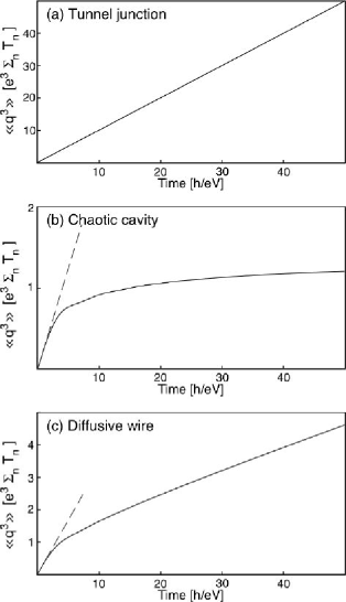
Figure 4: The third cumulant for (a) tunnel junction, (b) chaotic cavity and (c) diffusive wire at zero temperature. Both the tunnel junction and the diffusive wire show a linear growth at large $t$ due to non-vanishing zero-frequency value of $S_{\text{out,out,out}}$.

IV.2 A fully symmetrized three-current correlation function

A classical noise detector measures essentially a signal proportional to the symmetrized two-current correlation function

$$S_{\text{Symm}}^{(2)}(t_{1},t_{2})=\frac{1}{2}\big{\langle}\hat{I}(t_{1})\hat{I}(t_{2})+\hat{I}(t_{2})\hat{I}(t_{1})\big{\rangle}-\big{\langle}\hat{I}\big{\rangle}^{2}.$$ (38)

It is quite plausible to assume that a classical measurement of the third-order correlations would yield a signal proportional to what is essentially a generalization of (38), i.e., a fully symmetrized three-current correlation function golubev05

$$\begin{split}S_{\text{Symm}}^{(3)}(t_{1},t_{2},t_{3})&=\sum_{i\neq j\neq k=1}^{3}\big{\{}\frac{1}{16}\big{\langle}I(t_{i})T[I(t_{j})I(t_{k})]\big{\rangle}+\frac{1}{16}\big{\langle}\tilde{T}[I(t_{i})I(t_{j})]I(t_{k})\big{\rangle}\\ &\qquad\qquad\qquad-\frac{1}{2}\big{\langle}I(t_{i})\big{\rangle}\big{\langle}I(t_{j})I(t_{k})\big{\rangle}+\frac{1}{3}\big{\langle}I(t_{i})\big{\rangle}\big{\langle}I(t_{j})\big{\rangle}\big{\langle}I(t_{k})\big{\rangle}\big{\}}.\end{split}$$ (39)

This correlator is indeed symmetric in all permutations of the time arguments $t_{1}$, $t_{2}$, and $t_{3}$. We can then immediately rewrite the corresponding spectral function with the help of the in-out -ordering technique as

$$\begin{split}&S_{\text{Symm}}^{(3)}(\omega_{1},\omega_{2})\\ &=\frac{1}{2}S_{\rm in,out,out}(\omega_{1},\omega_{2})+\frac{1}{2}S_{\rm in,out,out}(\omega_{2}-\omega_{1},-\omega_{1})\\ &\quad+\frac{1}{2}S_{\rm in,out,out}(-\omega_{2},\omega_{1}-\omega_{2})+\frac{1}{2}S_{\rm out,out,in}(-\omega_{2},-\omega_{1})\\ &\quad+\frac{1}{2}S_{\rm out,out,in}(\omega_{1},\omega_{1}-\omega_{2})+\frac{1}{2}S_{\rm out,out,in}(\omega_{2}-\omega_{1},\omega_{2})\\ &\quad-S_{\rm out,out,out}(\omega_{1},\omega_{2}).\end{split}$$ (40)

Here the presence of various combinations of $\omega_{1}$ and $\omega_{2}$ is due to different orderings of the time arguments $t_{1}$, $t_{2}$, and $t_{3}$, and they also give rise to the hexagonal shape of the spectral function in the $(\omega_{1},\omega_{2})$–plane. This result is plotted in Fig. 3 (c) which coincides with the one found in Ref. golubev05 .

Comparing Eqs. (40) and (28), or Figs. 3 (c) and (a), we see that the symmetrized spectrum is generally quite different from the Keldysh contour ordered one. Nevertheless, the two coincide in the zero temperature, zero frequency limit such that $S_{\text{Symm}}^{(3)}(0,0)=\Gamma_{B}$ and hence corresponds to the usual third cumulant of full counting statistics.

IV.3 Three-current correlation functions of a multi-level quantum detector

As it is well-known aguado00 ; schoelkopf03 , two-level quantum detector responds to two-current correlators such that the direct transition rate to the higher level (absorption), given by the Fermi golden rule, is normally determined by the non-symmetrized spectral function

$$\begin{split}S_{\text{Q}}^{(2)}(\omega)=\int_{-\infty}^{\infty}dte^{i\omega t}\langle\delta\hat{I}(t)\delta\hat{I}(0)\rangle\end{split}$$ (41)

at the frequency $\omega=-\Delta\omega$, where $\Delta\omega$ is the level spacing. The corresponding relaxation rate (emission) is given by the same spectral function but now at the frequency $+\Delta\omega$. This result can be easily generalized to the case of a multilevel detector.

The next-higher order correction to the transition rate, which includes the effect of transitions via an intermediate state of a multi-level detector, depends, among others, on the three-current spectral function $S_{\text{Q}}^{(3)}(\omega_{1},\omega_{2})$, which was recently discussed in ojanen06 ; brosco06

$$\begin{split}S_{\text{Q}}^{(3)}(t_{1},t_{2},t_{3})=\frac{1}{(2\pi)^{2}}\int_{-\infty}^{\infty}d\omega_{1}d\omega_{2}e^{-i\omega_{1}(t_{1}-t_{2})}e^{-i\omega_{2}(t_{2}-t_{3})}S_{\text{Q}}^{(3)}(\omega_{1},\omega_{2}),\end{split}$$ (42)

where the partially time-ordered three-time current correlation function is

$$\begin{split}S_{\text{Q}}^{(3)}(t_{1},t_{2},t_{3})&=\langle\delta I(t_{1})T[\delta I(t_{2})\delta I(t_{3})]\rangle.\end{split}$$ (43)

We analyze this correlation function here using the in-out -ordering technique. Expanding in terms of in-out three current correlation functions yields

$$\begin{split}S_{\text{Q}}^{(3)}(t_{1},t_{2},t_{3})&=\langle\delta I_{\text{in}}(t_{1})\delta I_{\text{in}}(t_{2})\delta I_{\text{in}}(t_{3})-\delta I_{\text{in}}(t_{1})\delta I_{\text{out}}(t_{3})\delta I_{\text{in}}(t_{2})-\delta I_{\text{in}}(t_{1})\delta I_{\text{out}}(t_{2})\delta I_{\text{in}}(t_{3})\\ &\qquad+\delta I_{\text{in}}(t_{1})\delta I_{\text{out}}(t_{2})\delta I_{\text{out}}(t_{3})-\delta I_{\text{out}}(t_{1})\delta I_{\text{in}}(t_{2})\delta I_{\text{in}}(t_{3})+\delta I_{\text{out}}(t_{1})\delta I_{\text{out}}(t_{3})\delta I_{\text{in}}(t_{2})\\ &\qquad+\delta I_{\text{out}}(t_{1})\delta I_{\text{out}}(t_{2})\delta I_{\text{in}}(t_{3})-\delta I_{\text{out}}(t_{1})\delta I_{\text{out}}(t_{2})\delta I_{\text{out}}(t_{3})\rangle\end{split}$$ (44)

such that the corresponding spectral function is

$$\begin{split}S_{\text{Q}}^{(3)}(\omega_{1},\omega_{2})&=S_{\text{in,out,out}}(\omega_{1},\omega_{2})+S_{\text{out,out,in}}(\omega_{1},\omega_{1}-\omega_{2})+S_{\text{out,out,in}}(\omega_{1},\omega_{2})-S_{\text{out,out,out}}(\omega_{1},\omega_{2}),\end{split}$$ (45)

see Fig. 3 (d). The zero temperature, zero frequency limit of this quantity is given by $S_{\text{Q}}^{(3)}(0,0)=\Gamma_{B}$, i.e., it corresponds again to the usual third cumulant of current statistics.

IV.4 Discussion

Apart from the unordered spectral function Eq. (35), the various spectral functions discussed so far share many common features at zero temperature: (i) None of them contains the $S_{\text{out,in,out}}$ contribution. (ii) The sum of the terms containing 0, 1, 2, and 3 out-currents are given by binomial coefficients $(-1)^{k}\left(\begin{array}[]{c}3\\ k\end{array}\right)$, where $k$ is the number of out-currents. For energy-independent scattering, however, terms with $k=0,1$ vanish. (iii) Regions for which $|\omega_{1,2}|\geq eV/\hbar$ are only determined by the $k=2$ terms ($S_{\text{in,out,out}}$ and $S_{\text{out,out,in}}$) while the zero-frequency value is given by the $k=3$ term ($S_{\text{out,out,out}}$). (iv) In regions where $|\omega_{1,2}|\geq eV/\hbar$ the value of the spectral function is either zero or it saturates to a constant, unlike the two-current spectrum which increases linearly. The variously ordered spectral functions differ mainly from each other based on how the ’spectral power’ is distributed in the $(\omega_{1},\omega_{2})$–plane: the quantum detector noise $S_{\text{Q}}^{(3)}$ has twice the value of the symmetrized noise $S_{\text{Symm}}$, but that value is only achieved for $\omega_{1}>0$ while the symmetrized noise has the constant level everywhere in the $(\omega_{1},\omega_{2})$–plane, except in the hexagonal area bound within $|\omega_{1,2}|<eV/\hbar$.

V Conclusions

In this paper we have considered a formalism that facilitates calculation of time-ordered current correlation functions and applied it to current noise generated by a phase-coherent scatterer. Causality of the real-time representation of the scattering matrix causes products of in- and out-current operators, $\hat{I}_{\text{in}}(t_{1})$ and $\hat{I}_{\text{out}}(t_{2})$, to vanish if the in-current is taken later than the out-current; consequently, time-ordering of current operators may be expressed using in-out ordering, in which the out-current operators stand to the left of the in-currents, and vice versa for anti-time-ordering. The in-out ordering can be directly applied to current correlation functions of arbitrary order, and they can be directly evaluated in the case of thermal reservoirs. If the scattering matrix is, furthermore, energy-independent the correlation functions only depend on the transmission eigenvalues of the scatterer.

It is highly case-dependent to which particular current correlator a detector responds, and we evaluate three alternative functions. While a classical noise detector would respond to a fully symmetrized correlator, the spin detector discussed in the case of full counting statistics depends on the Keldysh-contour-ordered correlation function and a multi-level noise detector to a partially or fully time-ordered correlator. We obtain all the answers without cumbersome time-ordered integrations.

Appendix A Calculation of the three-current spectral functions with equilibrium reservoirs

We follow Ref. buttiker92 , and obtain all the three-current spectral functions needed by applying Wick’s theorem:

$$\begin{split}&\left\langle\left(\hat{a}_{k}^{\dagger}\hat{a}_{l}-\langle\hat{a}_{k}^{\dagger}\hat{a}_{l}\rangle\right)\left(\hat{a}_{m}^{\dagger}\hat{a}_{n}-\langle\hat{a}_{m}^{\dagger}\hat{a}_{n}\rangle\right)\left(\hat{a}_{p}^{\dagger}\hat{a}_{q}-\langle\hat{a}_{p}^{\dagger}\hat{a}_{q}\rangle\right)\right\rangle\\ &=\langle\hat{a}_{k}^{\dagger}\hat{a}_{q}\rangle\langle\hat{a}_{l}\hat{a}_{m}^{\dagger}\rangle\langle\hat{a}_{n}\hat{a}_{p}^{\dagger}\rangle-\langle\hat{a}_{k}^{\dagger}\hat{a}_{n}\rangle\langle\hat{a}_{l}\hat{a}_{p}^{\dagger}\rangle\langle\hat{a}_{m}^{\dagger}\hat{a}_{q}\rangle\\ &=\delta_{kq}\delta_{lm}\delta_{np}f_{k}(1-f_{m})(1-f_{p})-\delta_{kn}\delta_{lp}\delta_{mq}f_{k}f_{m}(1-f_{p}).\end{split}$$ (46)

Next we insert this result into the expression of a three-current correlation function, such as $\langle\delta\hat{I}_{L,\text{in}}(t_{1})\delta\hat{I}_{L,\text{in}}(t_{2})\delta\hat{I}_{L,\text{in}}(t_{3})\rangle$:

$$\begin{split}&\langle\delta\hat{I}_{L,\text{in}}(t_{1})\delta\hat{I}_{L,\text{in}}(t_{2})\delta\hat{I}_{L,\text{in}}(t_{3})\rangle\\ &=\frac{e}{h}\sum_{l}\int dE_{1}dE_{2}e^{i(E_{1}-E_{2})t_{1}/\hbar}\frac{e}{h}\sum_{n}\int dE_{3}dE_{4}e^{i(E_{3}-E_{4})t_{2}/\hbar}\frac{e}{h}\sum_{p}\int dE_{5}dE_{6}e^{i(E_{5}-E_{6})t_{3}/\hbar}\\ &\qquad\times\bigg{\langle}\left(\hat{a}^{\dagger}_{L,l}(E_{1})\hat{a}_{L,l}(E_{2})-\langle\hat{a}^{\dagger}_{L,l}(E_{1})\hat{a}_{L,l}(E_{2})\rangle\right)\left(\hat{a}^{\dagger}_{L,n}(E_{3})\hat{a}_{L,n}(E_{4})-\langle\hat{a}^{\dagger}_{L,n}(E_{3})\hat{a}_{L,n}(E_{4})\rangle\right)\times\\ &\qquad\qquad\qquad\times\left(\hat{a}^{\dagger}_{L,p}(E_{5})\hat{a}_{L,p}(E_{6})-\langle\hat{a}^{\dagger}_{L,p}(E_{5})\hat{a}_{L,p}(E_{6})\rangle\right)\bigg{\rangle}\\ &=-\left(\frac{e}{h}\right)^{3}\sum_{l}\int dE_{1}dE_{3}dE_{5}e^{i(E_{1}-E_{5})t_{1}/\hbar}e^{i(E_{3}-E_{1})t_{2}/\hbar}e^{i(E_{5}-E_{3})t_{3}/\hbar}f_{L}(E_{1})f_{L}(E_{3})(1-f_{L}(E_{5}))\\ &\quad+\left(\frac{e}{h}\right)^{3}\sum_{l}\int dE_{1}dE_{3}dE_{5}e^{i(E_{1}-E_{3})t_{1}/\hbar}e^{i(E_{3}-E_{5})t_{2}/\hbar}e^{i(E_{5}-E_{1})t_{3}/\hbar}f_{L}(E_{1})(1-f_{L}(E_{3}))(1-f_{L}(E_{5}))\\ &=\int\frac{d\omega_{1}}{2\pi}\frac{d\omega_{2}}{2\pi}e^{-i[\omega_{1}(t_{1}-t_{2})+\omega_{2}(t_{2}-t_{3})]}\\ &\qquad\qquad\times\frac{e^{3}}{h}N_{L}\int dE\ f_{L}(E)[1-f_{L}(E+\hbar\omega_{1})][1-f_{L}(E+\hbar\omega_{2})-f_{L}(E+\hbar\omega_{1}-\hbar\omega_{2})].\\ \end{split}$$ (47)

from which we can infer that

$$\begin{split}S_{\text{in,in,in}}(\omega_{1},\omega_{2})&=\frac{e^{3}}{h}N_{L}\int dE\ f_{L}(E)[1-f_{L}(E+\hbar\omega_{1})][1-f_{L}(E+\hbar\omega_{2})-f_{L}(E+\hbar\omega_{1}-\hbar\omega_{2})],\end{split}$$ (48)

cf. Eq. (21). We make next use of the following results valid for Fermi functions:

$$\begin{split}&\int dEf(E)[1-f(E+\delta E_{1})]=\frac{\delta E_{1}}{1-e^{-\beta\delta E_{1}}}\\ &\int dEf(E)[1-f(E+\delta E_{1})][1-f(E+\delta E_{2})]=\frac{1}{1-e^{-\beta\delta E_{1}}}\left[\frac{\delta E_{2}}{1-e^{-\beta\delta E_{2}}}-\frac{\delta E_{2}-\delta E_{1}}{1-e^{-\beta(\delta E_{2}-\delta E_{1})}}\right]\\ &\int dEf(E)[1-f(E+\delta E_{1})]f(E+\delta E_{2})=\frac{1}{1-e^{-\beta\delta E_{1}}}\bigg{[}\delta E_{1}-\frac{\delta E_{2}}{1-e^{-\beta\delta E_{2}}}+\frac{\delta E_{2}-\delta E_{1}}{1-e^{-\beta(\delta E_{2}-\delta E_{1})}}\bigg{]}.\\ \end{split}$$ (49)

The integration over energy $E$ can then be performed explicitly. In this particular case of $S_{\text{in,in,in}}(\omega_{1},\omega_{2})$, the energy integral contains Fermi functions of just one reservoir, and therefore its value vanishes:

$$\begin{split}\langle\delta\hat{I}_{L,\text{in}}(t_{1})\delta\hat{I}_{L,\text{in}}(t_{2})\delta\hat{I}_{L,\text{in}}(t_{3})\rangle=S_{\text{in,in,in}}(\omega_{1},\omega_{2})=0.\end{split}$$ (50)

This is generally true only for $S_{\text{in,in,in}}$ since it does not depend on the possibly energy-dependent scattering matrix. Spectral functions containing two in currents also have Fermi functions of just the left reservoir, but the energy-dependence of the scattering matrix may render the integrals non-zero. Yet in the case of energy-independent scattering such spectral functions vanish.

Appendix B In-out spectral functions of three currents

In Table 2 all the eight different three-current spectral functions are listed in the general case of energy-dependent scattering and assuming equilibrium reservoirs. The corresponding spectral functions for energy-independent scattering are given in Table 3, where $\{T_{n}\}$ denotes the set of energy-independent eigenvalues of the matrix $t^{\dagger}t$.

$$\begin{array}[]{rl}&S_{\text{in,in,in}}(\omega_{1},\omega_{2})=0\\ &S_{\text{in,in,out}}(\omega_{1},\omega_{2})\\ &=\frac{e^{3}}{h}\int{\rm d}E\ \bigg{\{}{\text{Tr}}[s^{\dagger}_{LL}(E+\hbar\omega_{2})s_{LL}(E)]f_{L}(E)[1-f_{L}(E+\hbar\omega_{1})][1-f_{L}(E+\hbar\omega_{2})]\\ &\qquad\qquad-{\text{Tr}}[s^{\dagger}_{LL}(E+\hbar\omega_{1})s_{LL}(E+\hbar\omega_{1}-\hbar\omega_{2})]f_{L}(E)[1-f_{L}(E+\hbar\omega_{1})]f_{L}(E+\hbar\omega_{1}-\hbar\omega_{2})]\bigg{\}}\\ &S_{\text{in,out,in}}(\omega_{1},\omega_{2})\\ &=\frac{e^{3}}{h}\int{\rm d}E\ \bigg{\{}{\text{Tr}}[s^{\dagger}_{LL}(E+\hbar\omega_{1})s_{LL}(E+\hbar\omega_{2})]f_{L}(E)[1-f_{L}(E+\hbar\omega_{1})][1-f_{L}(E+\hbar\omega_{2})]\\ &\qquad\qquad-{\text{Tr}}[s^{\dagger}_{LL}(E+\hbar\omega_{1}-\hbar\omega_{2})s_{LL}(E)]f_{L}(E)[1-f_{L}(E+\hbar\omega_{1})]f_{L}(E+\hbar\omega_{1}-\hbar\omega_{2})]\bigg{\}}\\ &S_{\text{out,in,in}}(\omega_{1},\omega_{2})\\ &=\frac{e^{3}}{h}\int{\rm d}E\ \bigg{\{}{\text{Tr}}[s^{\dagger}_{LL}(E)s_{LL}(E+\hbar\omega_{1})]f_{L}(E)[1-f_{L}(E+\hbar\omega_{1})][1-f_{L}(E+\hbar\omega_{2})]\\ &\qquad\qquad-{\text{Tr}}[s^{\dagger}_{LL}(E)s_{LL}(E+\hbar\omega_{1})]f_{L}(E)[1-f_{L}(E+\hbar\omega_{1})]f_{L}(E+\hbar\omega_{1}-\hbar\omega_{2})]\bigg{\}}\\ &S_{\text{in,out,out}}(\omega_{1},\omega_{2})\\ &=\frac{e^{3}}{h}\sum_{\alpha}\int dE\bigg{\{}{\text{Tr}}[s^{\dagger}_{LL}(E+\hbar\omega_{1})s_{L\alpha}(E+\hbar\omega_{2})s^{\dagger}_{L\alpha}(E+\hbar\omega_{2})s_{LL}(E)]f_{L}(E)[1-f_{L}(E+\hbar\omega_{1})][1-f_{\alpha}(E+\hbar\omega_{2})]\\ &\qquad\qquad-{\text{Tr}}[s^{\dagger}_{LL}(E+\hbar\omega_{1})s_{L\alpha}(E+\hbar\omega_{1}-\hbar\omega_{2})s_{L\alpha}^{\dagger}(E+\hbar\omega_{1}-\hbar\omega_{2})s_{LL}(E)]f_{L}(E)[1-f_{L}(E+\hbar\omega_{1})]f_{\alpha}(E+\hbar\omega_{1}-\hbar\omega_{2})]\bigg{\}}\\ &S_{\text{out,in,out}}(\omega_{1},\omega_{2})\\ &=\frac{e^{3}}{h}\sum_{\alpha}\int{\rm d}E\ \bigg{\{}{\text{Tr}}\left[s_{L\alpha}(E+\hbar\omega_{1})s^{\dagger}_{\alpha L}(E)s_{LL}(E+\hbar\omega_{1})s^{\dagger}_{LL}(E)\right]f_{\alpha}(E)(1-f_{L}(E+\hbar\omega_{1}))(1-f_{L}(E+\hbar\omega_{2}))\\ &\qquad\qquad-{\text{Tr}}\left[s_{LL}(E+\hbar\omega_{1})s^{\dagger}_{LL}(E)s_{L\beta}(E+\hbar\omega_{1})s^{\dagger}_{\beta L}(E)\right]f_{L}(E)(1-f_{\beta}(E+\hbar\omega_{1}))f_{L}(E+\hbar\omega_{1}-\hbar\omega_{2})\bigg{\}}\\ &S_{\text{out,out,in}}(\omega_{1},\omega_{2})\\ &=\frac{e^{3}}{h}\sum_{\alpha}\int dE\bigg{\{}{\text{Tr}}[s^{\dagger}_{LL}(E)s_{L\alpha}(E+\hbar\omega_{1})s^{\dagger}_{L\alpha}(E+\hbar\omega_{1})s_{LL}(E+\hbar\omega_{2})]f_{L}(E)[1-f_{\alpha}(E+\hbar\omega_{1})][1-f_{L}(E+\hbar\omega_{2})]\\ &\qquad\qquad-{\text{Tr}}[s^{\dagger}_{L\alpha}(E)s_{LL}(E+\hbar\omega_{1})s_{LL}^{\dagger}(E+\hbar\omega_{1}-\hbar\omega_{2})s_{L\alpha}(E)]f_{\alpha}(E)[1-f_{L}(E+\hbar\omega_{1})]f_{L}(E+\hbar\omega_{1}-\hbar\omega_{2})]\bigg{\}}\\ &S_{\text{out,out,out}}(\omega_{1},\omega_{2})\\ &=\frac{e^{3}}{h}\sum_{\alpha\beta\gamma}\int{\rm d}E\bigg{\{}{\text{Tr}}[s^{\dagger}_{L\alpha}(E)s_{L\beta}(E+\hbar\omega_{1})s^{\dagger}_{L\beta}(E+\hbar\omega_{1})s_{L\gamma}(E+\hbar\omega_{2})s_{L\gamma}^{\dagger}(E+\hbar\omega_{2})s_{L\alpha}(E)]\\ &\qquad\qquad\qquad\qquad\times f_{\alpha}(E)[1-f_{\beta}(E+\hbar\omega_{1})][1-f_{\gamma}(E+\hbar\omega_{2})]\\ &\qquad\qquad-{\text{Tr}}[s^{\dagger}_{L\alpha}(E)s_{L\beta}(E+\hbar\omega_{1})s^{\dagger}_{L\beta}(E+\hbar\omega_{1})s_{L\gamma}(E+\hbar\omega_{1}-\hbar\omega_{2})s_{L\gamma}^{\dagger}(E+\hbar\omega_{1}-\hbar\omega_{2})s_{L\alpha}(E)]\\ &\qquad\qquad\qquad\qquad\times f_{\alpha}(E)[1-f_{\beta}(E+\omega_{1})]f_{\gamma}(E+\omega_{1}-\omega_{2})]\bigg{\}}.\end{array}$$

Table 2: Three-current spectral functions for a general energy-dependent scatterer.

$$\begin{array}[]{ll}S_{\text{in,in,in}}(\omega_{1},\omega_{2})&=0\\ S_{\text{in,in,out}}(\omega_{1},\omega_{2})&=0\\ S_{\text{in,out,in}}(\omega_{1},\omega_{2})&=0\\ S_{\text{out,in,in}}(\omega_{1},\omega_{2})&=0\\ S_{\text{in,out,out}}(\omega_{1},\omega_{2})&=\frac{e^{3}}{h}\sum_{n}T_{n}(1-T_{n})\int dE\bigg{\{}f_{L}(E)[1-f_{L}(E+\hbar\omega_{1})][1-f_{R}(E+\hbar\omega_{2})]\\ &\qquad\qquad\qquad\qquad\qquad\qquad-f_{L}(E)[1-f_{L}(E+\hbar\omega_{1})]f_{R}(E+\hbar\omega_{1}-\hbar\omega_{2})]\bigg{\}}\\ S_{\text{out,in,out}}(\omega_{1},\omega_{2})&=\frac{e^{3}}{h}\sum_{n}T_{n}(1-T_{n})\int dE\bigg{\{}f_{R}(E)[1-f_{L}(E+\hbar\omega_{1})][1-f_{L}(E+\hbar\omega_{2})]\\ &\qquad\qquad\qquad\qquad\qquad\qquad-f_{L}(E)[1-f_{R}(E+\hbar\omega_{1})]f_{L}(E+\hbar\omega_{1}-\hbar\omega_{2})\bigg{\}}\\ S_{\text{out,out,in}}(\omega_{1},\omega_{2})&=\frac{e^{3}}{h}\sum_{n}T_{n}(1-T_{n})\int dE\bigg{\{}f_{L}(E)[1-f_{R}(E+\hbar\omega_{1})][1-f_{L}(E+\hbar\omega_{2})]\\ &\qquad\qquad\qquad\qquad\qquad\qquad-f_{R}(E)[1-f_{L}(E+\hbar\omega_{1})]f_{L}(E+\hbar\omega_{1}-\hbar\omega_{2})]\bigg{\}}\\ S_{\text{out,out,out}}(\omega_{1},\omega_{2})&=\frac{e^{3}}{h}\sum_{n}T_{n}(1-T_{n})^{2}\int dE\bigg{\{}f_{L}(E)[1-f_{L}(E+\hbar\omega_{1})][1-f_{R}(E+\hbar\omega_{2})-f_{R}(E+\hbar\omega_{1}-\hbar\omega_{2})]\\ &\qquad\qquad\qquad\qquad\qquad\qquad\qquad+f_{L}(E)[1-f_{R}(E+\hbar\omega_{1})][1-f_{L}(E+\hbar\omega_{2})-f_{L}(E+\hbar\omega_{1}-\hbar\omega_{2})]\\ &\qquad\qquad\qquad\qquad\qquad\qquad\qquad+f_{R}(E)[1-f_{L}(E+\hbar\omega_{1})][1-f_{L}(E+\hbar\omega_{2})-f_{L}(E+\hbar\omega_{1}-\hbar\omega_{2})]\bigg{\}}\\ &\quad+\frac{e^{3}}{h}\sum_{n}T_{n}^{2}(1-T_{n})\int dE\bigg{\{}f_{L}(E)[1-f_{R}(E+\hbar\omega_{1})][1-f_{R}(E+\hbar\omega_{2})-f_{R}(E+\hbar\omega_{1}-\hbar\omega_{2})]\\ &\qquad\qquad\qquad\qquad\qquad\qquad\qquad+f_{R}(E)[1-f_{L}(E+\hbar\omega_{1})][1-f_{R}(E+\hbar\omega_{2})-f_{R}(E+\hbar\omega_{1}-\hbar\omega_{2})]\\ &\qquad\qquad\qquad\qquad\qquad\qquad\qquad+f_{R}(E)[1-f_{R}(E+\hbar\omega_{1})][1-f_{L}(E+\hbar\omega_{2})-f_{L}(E+\hbar\omega_{1}-\hbar\omega_{2})]\bigg{\}}\end{array}$$

Table 3: Three-current spectral functions for an energy-independent scatterer.

References

- (1) Ya.M. Blanter and M. Büttiker, Phys. Rep. 336, 1 (2000).
- (2) R. Aguado and L.P. Kouwenhoven, Phys. Rev. Lett. 84, 1986 (2000).
- (3) R.J. Schoelkopf, A.A. Clerk, S.M. Girvin, K.W. Lehnert, and M.H. Devoret, in Ref. nazarov03 .
- (4) R. Deblock, E. Onac, L. Gurevich, and L.P. Kouwenhoven, Science 301, 203 (2003); P.-M. Billangeon, F. Pierre, H. Bouchiat, and R. Deblock, Phys. Rev. Lett. 96, 136804 (2006).
- (5) O. Astafiev, Yu.A. Pashkin, Y. Nakamura, T. Yamamoto, and J.S. Tsai, Phys. Rev. Lett. 93, 267007 (2004).
- (6) Y. Naveh, D.V. Averin, and K.K. Likharev, Phys. Rev. Lett. 79, 3482 (1997); Phys. Rev. B 59, 2848 (1999).
- (7) K.E. Nagaev, Phys. Rev. B 57, 4628 (1998). 176804 (2004).
- (8) K.E. Nagaev, S. Pilgram, and M. Büttiker, Phys. Rev. Lett. 92, 176804 (2004).
- (9) F.W.J. Hekking and J.P. Pekola, Phys. Rev. Lett. 96, 056603 (2006).
- (10) Quantum Noise in Mesoscopic Physics, edited by Yu. V. Nazarov (Kluwer, Dordrecht, 2003).
- (11) B. Reulet, J. Senzier and D. Prober, Phys. Rev. Lett. 91, 196601 (2003).
- (12) Yu. Bomze, G. Gershon, D. Shovkun, L.S. Levitov, and M. Reznikov, Phys. Rev. Lett. 95, 176601 (2005).
- (13) S. Gustavsson, R. Leturcq, B. Simovic, R. Schleser, T. Ihn, P. Studerus, K. Ensslin, D. C. Driscoll, and A. C. Gossard, Phys. Rev. Lett. 96, 076605 (2006).
- (14) S. Pilgram, K. E. Nagaev, and M. Büttiker, Phys. Rev. B 70, 045304 (2004).
- (15) L.S. Levitov and G.B. Lesovik, cond-mat/9401004 (unpublished).
- (16) L.S. Levitov, H. Lee, and G.B. Lesovik, J. Math. Phys. 37, 4845 (1996).
- (17) M. Büttiker, Phys. Rev. B 46, 12485 (1992).
- (18) G.B. Lesovik, Pis’ma Zh. Eksp. Teor. Fiz. 49, 513 (1989) [JETP Lett. 49, 592 (1989)].
- (19) B. Yurke and G.P. Kochanski, Phys. Rev. B 41, 8184 (1990).
- (20) M. Büttiker, Phys. Rev. Lett. 65, 2901 (1990).
- (21) C.W.J. Beenakker and H. Schomerus, Phys. Rev. Lett. 86, 700 (2001).
- (22) L.S. Levitov and M. Reznikov, Phys. Rev. B 70, 115305 (2004).
- (23) L.S. Levitov and G.B. Lesovik, Pis’ma Zh. Éksp. Teor. Fiz. 55, 534 (1992) [JETP Lett. 55, 555 (1992)].
- (24) G.B. Lesovik and N.M. Chtchelkatchev, Pis’ma Zh. Éksp. Teor. Fiz. 77, 464 (2003) [JETP Lett. 77, 393 (2003)].
- (25) A.V. Galaktionov, D.S. Golubev, and A.D. Zaikin, Phys. Rev. B 68, 085317 (2003); Phys. Rev. B 68, 235333 (2003).
- (26) K. Shepard, Phys. Rev. B 43, 11623 (1991).
- (27) M. Büttiker, A. Prêtre, and H. Thomas, Phys. Rev. Lett. 70, 4114 (1993).
- (28) D. Golubev, A.V. Galaktionov, and A.D. Zaikin, Phys. Rev. B 72, 205417 (2005).
- (29) T. Ojanen and T. T. Heikkilä, Phys. Rev. B 73, 020501(R) (2006).
- (30) V. Brosco, R. Fazio, F.W.J. Hekking, and J.P. Pekola, cond-mat/0603844 (unpublished).