The effect of the Abrikosov vortex phase on spin and charge states in magnetic semiconductor-superconductor hybrids

Abstract

We explore the possibility of using the inhomogeneous magnetic field carried by an Abrikosov vortex in a type-II superconductor to localize spin-polarized textures in a nearby magnetic semiconductor quantum well. We show how Zeeman-induced localization induced by a single vortex is indeed possible, and use these results to investigate the effect of a periodic vortex array on the transport properties of the magnetic semiconductor. In particular, we find an unconventional Integer Quantum Hall regime, and predict directly testable experimental consequences due to the presence of the periodic spin polarized structure induced by the superconducting vortex lattice in the magnetic semiconductor.

I Introduction

The possibility of exploring both charge and spin degrees of freedom in carriers has attracted the attention of the condensed matter community in recent years. The discovery of ferromagnetism in diluted magnetic semiconductors (DMS) like GaMnAs Ohno (1996), opened the opportunity to explore precisely such independent spin and charge manipulations. A fundamental property of diluted magnetic semiconductors (DMS) (both new III-Mn-V and the more established II-Mn-VI systems) is that a relatively small external magnetic field can cause enormous Zeeman splittings of the electronic energy levels, even when the material is in the paramagnetic state Furdyna (1988); Lee (2000). This feature can be used in spintronics applications as it allows separating states with different spin. For instance, Fiederling et al. had successfully used a II-Mn-VI DMS under effect of low magnetic fields in spin-injection experiments  Fiederling et al. (1999).

Another utilization of this feature has been discussed by us Berciu and Janko (2003); Redlinski et al. (2005a, b); Berciu et al. (2005): Due to the giant Zeeman splitting, a magnetic field with considerable spatial variation can be a very effective confining agent for spin polarized carriers in these DMS systems.

Producing a non-uniform magnetic field with nanoscale spatial variation inside DMS systems can be an experimental challenge. One option is the use of nanomagnets deposited on the top of a DMS layer. In fact, nanomagnets have already been used as a source of non-homogeneous magnetic field Peeters and Matulis (1993); Freire et al. (2000). Freire et al. Freire et al. (2000), for example, have analyzed the case of a normal semiconductor in the vicinity of nanomagnets. In such case, the non-homogeneous magnetic field modifies the exciton kinetic-energy operator and can weakly confine excitons in the semiconductor. In contrast, we have examined a DMS in the vicinity of nanomagnets with a variety of shapes Berciu and Janko (2003); Redlinski et al. (2005a, b). In these cases, the confinement is due the Zeeman interaction which is hundreds of times stronger than the variation of kinetic-energy in DMS.

Another possibility for obtaining the inhomogeneous magnetic fields is the use of superconductors. Nanoscale field singularities appear naturally in the vortex phase of superconducting (SC) films. Above the lower critical field B${}_{c_{1}}$, in the Abrikosov vortex phase, superconducting vortices populate the bulk of the sample, forming a flux lattice, each vortex carrying a quantum of magnetic flux $\phi_{0}/2=h/(2e)$. The field of a single vortex is non-uniformly distributed around a core of radius $r\sim\xi$ (where $\xi$ is the coherence length) decaying away from its maximum value at the vortex center over a length scale $\lambda$ (where $\lambda$ is the penetration depth).

A regular two dimensional electron gas (2DEG) in the vicinity of superconductors in a vortex phase has already been the subject of both theoretical Rammer and Shelankov (1987); Brey and Fertig (1993); Chang and Niu (1994); Nielsen and Hedegrd (1995); Gumbs et al. (1995); Oh (1999); Matulis and Peeters (2000); Wang et al. (2004) and experimental studies Bending et al. (1990); Geim et al. (1992); Danckwerts et al. (2000). In this context, because the Landé $g$ factor (and thus the Zeeman interaction) is very small in normal semiconductors, the main consequence of the inhomogeneous magnetic fields is a change in the kinetic-energy term of the Hamiltonian. The flux tubes do not produce bound states, but act basically as scattering centers Bending et al. (1990); Nielsen and Hedegrd (1995). The Zeeman interaction was either neglected or treated as a small perturbation whose main consequence was to broaden the already known Hofstadter butterfly subbands.

In the work presented here, we consider the case where the 2DEG is confined inside a DMS. Due to the giant Zeeman interaction in paramagnetic DMSs (whose origin is briefly explained in Section II), the Zeeman interaction becomes the dominant term in these systems, leading to appearance of bound states inside the flux tubes. These play a central role in our work and qualitatively change the nature of the magnetotransport in these systems, compared to the ones previously studied.

In this article we study a SC film deposited on top of a diluted magnetic semiconductor quantum well under the influence of an external magnetic field $\vec{B}_{0}=B_{0}\vec{e}_{z}$ (see Fig. 1), for all values of $B_{0}$ between the two possible asymptotic limits. For very low applied fields, the SC film is populated with few isolated vortices, each vortex producing a highly inhomogeneous magnetic field which localizes spin polarized states in the DMS. In section III we obtain numerically the energy spectrum and the wave functions for the bound states localized by the vortex field of an isolated vortex in the DMS QW.

However, the main advantage of using SC vortices to generate confining potentials in the DMSs is the possibility of varying the distance between them by adjusting the external magnetic field. For increasing values of the external magnetic field $B_{0}$, the vortices in the SC are organized in a triangular lattice. The lattice spacing $a$ is related to the applied magnetic field by $B_{0}=\phi_{0}/(\sqrt{3}a^{2})$. In this limit, the triangular vortex lattice in the SC leads to a periodically modulated magnetic field inside the neighboring DMS layer.

Since the magnetic field produced by the SC flux lattice creates an effective spin dependent confinement potential for the carriers in the DMS, the properties of the superconductors will be reflected in the energy spectrum of the DMS. In particular, as the lattice spacing and spatial dependence of the non-uniform magnetic field (our confining potentials) change with $B_{0}$, we have a peculiar system in the DMS where both the lattice spacing and the depth of the potentials are modified by an applied magnetic field.

For low external magnetic fields, the overlap between the magnetic fields of independent vortices is small and as a consequence, the giant Zeeman effect produces deep effective potentials. The trapped states of the isolated vortex discussed in section III widen into energy bands of spin polarized states. The width of the bands is defined by the exponentially small hopping $t$ between neighboring trapped states. However, since the flux through each unit cell is $\phi/\phi_{0}=q/p=1/2$, the energy bands will be those of a triangular Hofstadter butterfly Claro and Wannier (1979). As long as the hopping $t$ is small compared to the spacing between consecutive trapped states, this Hofstadter problem corresponds to the regime of a dominant periodic modulation, which can be treated within a simple tight-binding model Hofstadter (1976); Claro and Wannier (1979) and each band is expected to split into $p$ (in this case, $p=2$) magnetic subbands. This band-structure has unique signatures in the magnetotransport, as discussed below. Its measurement would provide a clear signature of the Hofstadter butterfly, which is currently a matter of considerable experimental interest Schlosser et al. (1996); Albrecht et al. (2001); Melinte et al. (2004).

On the other hand, for a high applied external magnetic field $B_{0}$, the magnetic fields of different vortices begin to overlap significantly. In this limit, the total magnetic field in the DMS layer is almost homogeneous. Its average is $B_{0}\vec{e}_{z}$, but it has a small additional periodic modulation (the same effect can be achieved at a fixed $B_{0}$ by increasing the distance $z$ between the SC and DMS layers). For such quasi-homogeneous magnetic fields, the Zeeman interaction can no longer induce trapping; instead it reverts to its traditional role of lifting the spin degeneracy. The small periodic modulation insures the fact that the system still corresponds to a $\phi/\phi_{0}=1/2$ Hofstadter butterfly, but now in the other asymptotic limit, namely that of a weak periodic modulation. In this case, each Landau level is expected to split into $q$ subbands, with a bandwidth controlled by the amplitude of the weak modulation. The case $\phi/\phi_{0}=1/2$ has $q=1$ and there are no additional gaps in the bandstructure. As a result, one expects to see the usual IQHE in magnetotransport in this regime. To summarize, as long as there is a vortex lattice, the setup corresponds to a $\phi/\phi_{0}=1/2$ Hofstadter butterfly irrespective of the value of external magnetic field $B_{0}$. Instead, $B_{0}$ controls the amplitude of the periodic modulation, from being the large energy scale (small $B_{0}$) to being a small perturbation (large $B_{0}$).

In section IV, we use a unified theoretical approach to analyze how the 2-D modulated magnetic field produced by the vortex lattice affects the free carries in the DMS QW, and the resulting bandstructures. We obtain the energy spectrum going from the asymptotic limit of a very small periodic modulation to the asymptotic limit of isolated vortices. In the later case, we are able to reproduce the results obtained in the Section III.

As one of the most direct signatures of the Hofstadter butterfly, in Section V we discuss the fingerprints of the band structures obtained in section IV on the magnetotransport properties of these 2DEG, in particular their Hall (transversal) conductance. This is shown to change significantly as one tunes the external magnetic field between the two asymptotic limits. Finally, in Section VI we discuss the significance of these results.

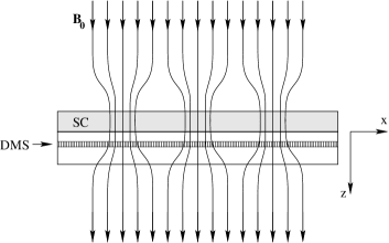
Figure 1: Sketch of the type-II SC - DMS heterostructure in a uniform external magnetic field.

II Giant Zeeman effect in paramagnetic Diluted Magnetic Semiconductors

One of the most remarkable properties of the DMS is the giant Zeeman effect they exhibit in their paramagnetic state, with effective Landé factors of the charge carriers on the order of 10² - 10³. Since this effect plays a key role in determining the phenomenology we analyze in this work, we briefly review its origin in this section, using a simple mean-field picture.

The exchange interaction of an electron with the impurity spins $\vec{S}_{i}$ located at positions $\mathbf{R}_{i}$, is:

$$H_{ex}=\sum_{i}J(\vec{r}-\vec{R}_{i})\vec{S}_{i}\cdot\vec{s}.$$ (1)

where $J(\vec{r})$ is the exchange interaction. Within a mean-field approximation (justified since each carrier interacts with many impurity spins) $\vec{S}_{i}\cdot\vec{s}\rightarrow\langle\vec{S}_{i}\rangle\vec{s}+\vec{S}_{i}\langle\vec{s}\rangle$, and the average exchange energy felt by the electron becomes:

$$E_{ex} = N_{0}x\alpha\langle\vec{S}\rangle\vec{s}$$ (2)

Here, $x$ is the molar fraction of Mn dopants, $N_{0}$ is the number of unit cells per unit volume, $\langle\vec{S}\rangle$ is the average expectation value of the Mn spins, and $\alpha=\int d\vec{r}u^{*}_{c,\vec{k}=0}(\vec{r})J(\vec{r})u_{c,\vec{k}=0}(\vec{r})$ is an integral over one unit cell, with $u_{c,\vec{k}=0}(\vec{r})$ being the periodic part of the conduction band Bloch wave-functions. The usual virtual crystal approximation, which averages over all possible location of Mn impurities, has been used. Exchange fields for holes can be found similarly; they are somewhat different due to the different valence-band wave-functions.

In a ferromagnetic DMS, this terms explains the appearance of a finite magnetization below $T_{C}$: as the Mn spins begin to polarize, $\langle\vec{S}\rangle\neq 0$, this exchange interaction induces a polarization of the charge carrier spins $\langle\vec{s}\rangle\neq 0$. In turn, exchange terms like $\vec{S}_{i}\langle\vec{s}\rangle$ further polarize the Mn, until self-consistency is reached.

In paramagnetic DMS, however, $\langle\vec{S}\rangle=0$ and charge carrier states are spin-degenerate. The spin-degeneracy can be lifted if an external magnetic field $\vec{B}$ is applied. Of course, the usual Zeeman interaction $-g\mu_{B}\vec{s}\cdot\vec{B}$ is present, although this is typically very small. Much more important is the indirect coupling of the charge carrier spin to the external magnetic field, mediated by the Mn spins. The origin of this is the exchange energy of Eq. (2), and the fact that in an external magnetic field, the impurity spins acquire a finite polarization $\langle\vec{S}\rangle\parallel\vec{B}$, $|\langle\vec{S}\rangle|=S{\cal B}_{S}(g\mu_{B}SB/(k_{B}T))$, where $S$ is the value of the impurity spins ($5/2$ for Mn) and ${\cal B}_{S}$ is the Brillouin function (for simplicity of notation, we assume the same bare $g$-factor for both charge carriers and Mn spins; also, here we neglect the supplementary contribution coming from the $\vec{S}_{i}\langle\vec{s}\rangle$ terms, since typically an impurity spin interacts with few charge carriers). The total spin-dependent interaction of the charge-carriers is, then:

$${\cal H}_{ex}=-g\mu_{B}\vec{s}\cdot\vec{B}+N_{0}x\alpha\langle\vec{S}\rangle\vec{s}=g_{\rm eff}\mu_{B}\vec{s}\cdot\vec{B}$$ (3)

where

$$g_{\rm eff}=-g+\frac{N_{0}x\alpha}{\mu_{B}B}S{\cal B}_{S}\left(\frac{g\mu_{B}SB}{k_{B}T}\right)$$ (4)

for electrons, with an equivalent expression for holes. For low magnetic fields, $g_{\rm eff}$ becomes independent of the value of $B$, although it is a function of $T$ and $x$. Its large effective value is primarily due to the strong coupling $\alpha$ (large $J(\vec{r})$) between charge carriers and Mn spins.

In the calculations shown here, we use as DMS parameters an effective charge-carrier mass $m=0.5m_{e}$ and $g_{\rm eff}=500$, unless otherwise specified. Such values are reasonable for holes in several DMS, such as GaMnAs and CdMnTe.

III Isolated vortex

In this section we discuss the case where the free carriers in a narrow DMS quantum well are subjected to the magnetic field created by a single SC vortex. This situation is relevant for very low applied fields, when the density of SC vortices is very low.

We first need to know the magnetic field induced by the SC vortex in the DMS QW. For an isotropic superconductor, this problem was solved by Pearl Pearl (1964). The field outside of the SC is the free space solution matching the appropriate boundary conditions at the SC surface. Let $r=\sqrt{x^{2}+y^{2}}$ be the radial distance measured from the vortex center, while $z$ is the distance away from the edge of the superconductor (here, $z$ is the distance between the SC film and the DMS QW, see Fig. 1). The radial and transversal components of the magnetic field created by a single vortex in the DMS layer are Pearl (1964); Kirtley et al. (1999); Carneiro and Brandt (2000); Brandt (1995):

$$B^{(v)}_{r}(r,z)=\frac{\phi_{0}}{4\pi\lambda^{2}}\int_{0}^{\infty}{kdk\frac{J_{1}(kr)\exp(-kz-\frac{1}{2}\xi^{2}k^{2})}{\tau(k+\tau)}}$$ (5)

$$B^{(v)}_{z}(r,z)=\frac{\phi_{0}}{4\pi\lambda^{2}}\int_{0}^{\infty}{kdk\frac{J_{0}(kr)\exp(-kz-\frac{1}{2}\xi^{2}k^{2})}{\tau(k+\tau)}}$$ (6)

$\phi_{0}=h/e$ is the quantum of magnetic flux, $\lambda$ and $\xi$ are the penetration depth and the correlation length of the superconductor, $\tau=\sqrt{k^{2}+\lambda^{-2}}$ and $J_{\nu}(\zeta)$ are Bessel functions. The term $e^{-\frac{1}{2}\xi^{2}k^{2}}$ is a cut-off introduced in order to account for the effects of the finite vortex core size, which are not included in the London theoryBrandt (1995).

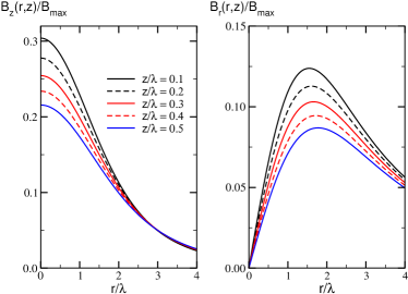
Figure 2: The transversal (left) and radial (right) components of the magnetic field created by a single vortex in Nb ($\xi=35$ nm, $\lambda=40$ nm), at different distances $z$ (in units of $\lambda$). $B_{\rm max}={\phi_{0}}/{(4\pi\lambda^{2})}\sim 0.207$ T.

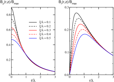
Figure 3: The transversal (left) and radial (right) components of the magnetic field created by a single vortex at a distance z=0.1$\lambda$, for different values of the coherence length (in units of $\lambda$. Here, $\lambda=40$ nm and $B_{\rm max}={\phi_{0}}/{(4\pi\lambda^{2})}\sim 0.207$ T.

In Figs. 2 and 3 we show typical magnetic field distributions for different ratios of $\xi/\lambda$ and of $z/\lambda$. As expected, the transversal component is largest under the vortex core, and decreases with increasing $z$ (see Fig. 2). The radial component is zero for $r=0$, has a maximum for $r\sim\xi$ and then decays fast. This magnetic field is qualitatively similar to that created by cylindrical nanomagnets Berciu and Janko (2003). The field distribution depends significantly on the properties of the SC. Its maximum value is bounded by $B_{max}={\phi_{0}}/{(4\pi\lambda^{2})}$. For a fixed $\lambda$, higher values of $B$ and larger gradients (which are desirable for our problem) occur for smaller ratios $\xi/\lambda$ (see Fig. 3). It follows that the ideal SC candidates would be extreme type-II (with $\xi/\lambda\ll 1$), and also have small penetration depths $\lambda$. In order to avoid unnecessary complications due to pinning, the superconductor should also have low intrinsic pinning (e.g., NbSe₂ Bhattacharya and Higgins (1993) or MgB₂ Bugoslavsky et al. (2001)). Incidentally, NbSe₂ is also attractive since it was shown that it can be deposited via MBE onto GaAs Yamamoto et al. (1994). In the calculations shown here, we use SC parameters characteristic of Nb: $\lambda=40\ {\rm nm}$, $\xi=35{\rm nm}$.

We now analyze the effects of this magnetic field on the DMS charge carriers. Using a parabolic band approximation, the effective Hamiltonian of a charge carrier inside the DMS QW, in the presence of the magnetic field $\vec{B}^{(v)}(r,z)$ of the SC vortex, is [see Eq. (3)]:

$${\cal H}={1\over 2{m}}\left[\vec{p}-q\vec{A}^{(v)}(r,z)\right]^{2}-{1\over 2}g_{\rm eff}\mu_{B}\vec{\sigma}\cdot\vec{B}^{(v)}(r,z)$$ (7)

where $m$ and $q$ are the effective mass and the charge of the carrier, and $\vec{A}^{(v)}(r,z)$ is the vector potential, $\vec{B}^{(v)}(r,z)=\nabla\times\vec{A}^{(v)}(r,z)$. For simplicity, we consider a narrow QW, so that the motion is effectively two-dimensional. As a result, $z$ is just a parameter controlling the value of the magnetic field. Generalization to a finite width QW has no qualitative effects.

As discussed in Ref. Berciu and Janko, 2003, for a dipole-like magnetic field such as the one created by the isolated SC vortex, the eigenfunctions have the general structure:

$$\psi_{\rm m}(r,\phi)=\exp{(i{\rm m}\phi)}\left(\begin{array}[c]{c}\psi_{\uparrow}^{({\rm m})}(r)\\ \psi_{\downarrow}^{({\rm m})}(r)\exp{[i\phi]}\\ \end{array}\right)$$ (8)

where ${\rm m}$ is an integer and $\phi=\tan^{-1}(y/x)$ is the polar angle. The radial equations satisfied by the up and down spin components can be derived straightforwardly:

$$\left[\!-\frac{1}{r}\!\frac{d}{dr}\!\left(\!r\frac{d}{dr}\!\right)+\!\frac{{\rm m}^{2}}{r^{2}}-\tilde{g}b_{z}(r)-e\right]\!\!\psi_{\uparrow}(r)=\tilde{g}b_{r}(r)\psi_{\downarrow}(r)$$

$$\left[\!-\frac{1}{r}\!\frac{d}{dr}\!\left(\!r\frac{d}{dr}\!\right)\!+\!\frac{({\rm m}\!+\!1)^{2}}{r^{2}}\!+\!\tilde{g}b_{z}(r)\!-\!e\right]\!\!\psi_{\downarrow}(r)\!=\!\tilde{g}b_{r}(r)\psi_{\uparrow}(r)$$

all lengths are in units of $\lambda$. The unit of energy is $E_{0}={\hbar^{2}}/(2m\lambda^{2})=0.05$ meV if we use $m=0.5m_{e}$ and $\lambda=40$ nm. $e=E/E_{0}$ is the eigenenergy. The magnetic fields have been rescaled, $\vec{B}^{(v)}(r,z)=\phi_{0}/(4\pi\lambda^{2})\cdot\vec{b}(r)$ (from now on, the distance $z$ between the DMS and QW is no longer explicitly specified). Finally, $\tilde{g}=g_{\rm eff}\mu_{B}\phi_{0}/(8\pi\lambda^{2}E_{0})=g_{\rm eff}/8$ if $m=0.5m_{e}$. The $\vec{A}^{(v)}(\vec{r})$ terms were left out. This is justified since they are negligible compared to the Zeeman term, which is enhanced by $g_{\rm eff}\sim 10^{2}$ (this was verified numerically). The bound eigenstates $e<0$ are found numerically, by expanding the up and down spin components in terms of a complete basis set of functions (cubic B-splines).

The energies of the ground state (${\rm m}=0$) and the first two excited trapped states (${\rm m}=\pm 1$) are shown in Fig. 4, as a function of (a) the ratio $\xi/\lambda$, (b) the distance $z/\lambda$ to the quantum well, and (c) the ratio $g_{\rm eff}m/m_{e}$. As expected, the binding energies are largest when the magnetic fields and therefore the Zeeman potential well are largest, in the limit $z\rightarrow 0$ and $\xi/\lambda\rightarrow 0$. Since $\xi/\lambda$ controls the spatial extent of the Zeeman trap, the distance between the ground and first excited states increase for decreasing $\xi/\lambda$. All binding energies increase basically linearly with increasing $g_{\rm eff}$.

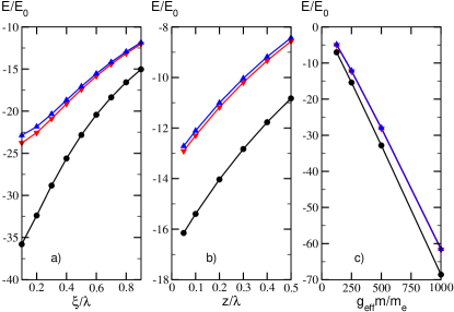
Figure 4: Energy of the ground state (circles) and of the first two excited states (triangles), for a charge carrier trapped in the Zeeman potential created by an isolated vortex, as a function of (a) the coherence length of the SC; here $z=0.1\lambda$, $m=0.5m_{e}$ and $g_{\rm eff}=500$; (b) the distance between the DMS layer and the SC. Here $\xi/\lambda=35/40$, and the other parameters are as in (a); and (c) the value of $g_{\rm eff}m/m_{e}$. Here $\xi/\lambda=35/40$. In all cases, $E_{0}=\hbar^{2}/(2m\lambda^{2})=0.05$ meV, for $\lambda=40$ nm.

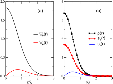
Figure 5: (a)$\psi^{(0)}_{\uparrow}(r)$ and $\psi^{(0)}_{\downarrow}(r)$ of Eq. (8), for the ground-state, when $z=0.1\lambda$(b) The corresponding density of charge $\rho(r)=|\psi^{(0)}_{\uparrow}(r)|^{2}+|\psi^{(0)}_{\downarrow}(r)|^{2}$, transversal spin density $s_{z}(r)={1\over 2}(|\psi^{(0)}_{\uparrow}(r)|^{2}-|\psi^{(0)}_{\downarrow}(r)|^{2})$ and radial spin density $s_{r}(r)={\rm Re}(\psi^{(0)*}_{\downarrow}(r)\psi^{(0)}_{\uparrow}(r))$.

The ground-state wavefunction, corresponding to ${\rm m}=0$ in Eq. (8), is shown in Fig. 5a. While $\psi^{(0)}_{\downarrow}(r)\neq 0$ because of the presence of the radial component, its value is significantly smaller than that of the spin-up component $\psi^{(0)}_{\uparrow}(r)$ which is favored by the Zeeman interaction with the large transversal magnetic field. The expectation value of the trapped charge carrier spin has a “hedgehog”-like structure, primarily polarized along the $z$-axis, but also having a small radial component (see Fig. 5b). The general structure of these eigenfunctions [Eq. (8)] has been shown to be responsible for allowing coupling to only one circular polarization of photons which are normally incident on the DMS layer, suggesting possible optical manipulation of these trapped, highly spin-polarized charge carriers Berciu and Janko (2003). After using quite drastic analytic simplifications, the results of Ref. Berciu and Janko (2003) also suggested that depending on the orientation (sign) of the $B_{z}$ component, only one set of excited state (either ${\rm m>0}$ or ${\rm m<0}$) is present. Numerically, we find both sets of states present, with a small lifting of their degeneracy.

IV Two-dimensional vortex lattice

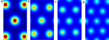
Figure 6: Modulation of the transversal component of the magnetic field $\vec{B}_{L}(\vec{r};z)$ of the flux lattice in a given area of a type II superconductor, for an applied external field $B_{0}=0.07$ T, $B_{0}=0.10$ T, $B_{0}=0.15$ T and $B_{0}=0.19$ T respectively in (a), (b), (c) and (d). As the applied field $B_{0}$ increases, the distance between vortices and the modulation of the total field decreases.

When placed in a finite external magnetic field $B_{c1}<B_{0}<B_{c2}$, the SC creates a finite density of vortices arranged in an ordered triangular lattice Abrikosov (1957). Since each unit cell encloses the magnetic flux $B_{0}a^{2}\sqrt{3}/2=\phi_{0}/2$ of its vortex, the lattice constant $a\sim 1/\sqrt{B_{0}}$ is controlled by the external field $B_{0}$, see Fig. 6. Consequently, $a$ can be varied considerably, depending on the ratio $T/T_{C}$ of the temperature $T$ to the SC critical temperature $T_{C}$, which sets the value of $B_{c1}$, and the ratio $B_{0}/B_{c1}$. The corresponding Hamiltonian for the free carriers in the DMS quantum well, in the presence of a SC vortex lattice, is given by:

$${\cal H}={1\over 2m}\left[\vec{p}+e\vec{A}_{L}(\vec{r};z)\right]^{2}-{1\over 2}g_{\rm eff}\mu_{B}\vec{\sigma}\cdot\vec{B}_{L}(\vec{r};z)$$ (9)

Here, $-e$ is the charge of the charge carriers, assumed to be electrons. Holes can be treated similarly. We use $\vec{r}=(x,y)$ to describe the 2D position of the charge carrier inside the narrow (2D) DMS QW. The magnetic field $\vec{B}_{L}(\vec{r})$ created by the triangular vortex lattice is the sum of the fields created by single vortices [see Eqs. (5), (6)]:

$$\vec{B}_{\rm L}(\vec{r};z)=\sum_{\vec{R}}\vec{B}^{(v)}(\vec{r}-\vec{R};z)=B_{0}\hat{z}+\sum_{\vec{G}\neq 0}e^{i\vec{G}\cdot\vec{r}}\vec{B}_{\vec{G}}(z)$$ (10)

where the triangular lattice is defined by $\vec{R}=na(1,0)+m{a\over 2}(1,\sqrt{3})$, $n,m\in Z$, and $\vec{G}$ are the reciprocal lattice vectors. The first term is the average field per unit cell, which equals the applied external field $B_{0}\hat{z}$. The second term is the periodic field induced by the screening supercurrents. This term has zero flux through any unit cell and decreases rapidly as the distance $z$ between the SC and the DMS layers increases. As in the previous section, $z$ is here just a parameter, and we will not write it explicitly from now on.

Likewise, we separate the vector potential in two parts, corresponding to each contribution of the magnetic field:

$$\vec{A}_{\rm L}(\vec{r})=\vec{A}_{0}(\vec{r})+\vec{a}(\vec{r}).$$

In the Landau gauge, $\vec{A}_{0}(\vec{r})=(0,B_{0}x,0)$ and $\vec{a}(\vec{r})=\sum_{\vec{G}\neq 0}e^{i\vec{G}\cdot\vec{r}}\vec{a}_{\vec{G}}$, with $a_{\vec{G}}=[i\vec{G}\times\vec{B}_{\bar{G}}(z)]/|\vec{G}|^{2}$.

Before constructing the solutions for the full Hamiltonian of Eq. (9), we first briefly review the solutions in the presence of only a homogeneous field $B_{0}$, in order to fix the notation. In this case the Zeeman term lifts the spin degeneracy, but it is the orbital coupling that essentially determines the energy spectrum of the carriers, which consists of spin-polarized Landau Levels (LL):

$$E_{N,\sigma}=\hbar\omega_{c}\left(N+{1\over 2}\right)-{1\over 2}g_{\rm eff}\mu_{B}B_{0}\sigma.$$ (11)

In the Landau gauge the corresponding eigenstates are:

$$\phi_{N,k_{y},\sigma}(\vec{r})={e^{ik_{y}y}e^{-{1\over 2}\left({x\over l}+lk_{y}\right)^{2}}\over\sqrt{b}\sqrt{l\sqrt{\pi}2^{N}N!}}H_{N}\left({x\over l}+lk_{y}\right)\chi_{\sigma},$$ (12)

where $l=\sqrt{\hbar/(eB_{0})}$ is the magnetic length and $\omega_{c}=eB_{0}/m$ is the cyclotron frequency. $N\geq 0$ is the index of the LL, $H_{N}(\zeta)$ are Hermite polynomials and $k_{y}$ is a momentum. $\chi_{\sigma}$ are spin eigenstates, $\sigma_{z}\chi_{\sigma}=\sigma\chi_{\sigma}$, $\sigma=\pm 1$. Each LL is highly degenerate and can accommodate up to one electron per $2\pi l^{2}$ sample area. The filling factor $\nu=n2\pi l^{2}$, where $n$ is the 2D electron density in the DMS QW, counts how many LL are fully or partially filled.

This spectrum of highly degenerate LLs is very different from that arising if only the periodic part of the magnetic field and vector potentials are present in the Hamiltonian. In this case, the system is invariant to the discrete lattice translations. As a result, one finds the spectrum to consist of electronic bands defined in a Brillouin zone determined by the periodic Zeeman potential, the eigenfunctions being regular Bloch states. One can roughly think of these states as arising from nearest-neighbor hopping between the states trapped under each individual vortex, discussed in the previous section.

In order to construct solutions that include both the periodic and the homogeneous part of the magnetic field, we need to first consider the symmetries of Hamiltonian (9). Because of the orbital coupling to the non-periodic part of the vector potential $\vec{A}_{0}$, the ordinary lattice translation operators $T(\vec{R})=e^{{i\over\hbar}\vec{R}\cdot\vec{p}}$ do not commute with the Hamiltonian. Instead, one needs to define so-called magnetic translation operators Zak (1964):

$$T_{M}(\vec{R})=e^{-{ie\over\hbar}B_{0}R_{x}y}e^{{i\over\hbar}\vec{R}\cdot\vec{p}}.$$

It is straightforward to verify that these operators commute with the Hamiltonian, $[{\cal H},T_{M}(\vec{R})]=0$, and that

$$T_{M}(\vec{R})T_{M}(\vec{R^{\prime}})=e^{-{ie\over\hbar}B_{0}R^{\prime}_{x}R_{y}}T_{M}(\vec{R}+\vec{R^{\prime}}).$$

It follows that these operators form an Abelian group provided that we define a magnetic unit cell so that the magnetic flux through it is an integer multiple of $\phi_{0}$. In our case, as already discussed, the magnetic flux through the unit cell of the vortex lattice is precisely $\phi_{0}/2$. We therefore define the magnetic unit cell to be twice the size of the original one. We use a rectangular unit cell, as shown in Fig. 7a. The new lattice vectors are $\vec{a}=(a,0)$ and $\vec{b}=(0,b)$, with $b=a\sqrt{3}$, and $\vec{R}_{nm}=n\vec{a}+m\vec{b}$. The basis consists of two vortices, one placed at the origin and one placed at $\vec{\delta}=(\vec{a}+\vec{b})/2$. The associated magnetic Brillouin zone is $k_{x}\in(-\pi/a,\pi/a];k_{y}\in(-\pi/b,\pi/b]$ and the reciprocal magnetic lattice vectors are $\vec{G}_{n,m}=n(2\pi/a)\hat{x}+m(2\pi/b)\hat{y}$, $n,m\in Z$ (see Fig. 7b).

Figure 7: (a) Rectangular magnetic unit cell containing 2 vortices, and its lattice vectors. (b) The associated magnetic Brillouin zone and the location of the special, high-symmetry points $\Gamma$, X and M.

With this choice, the wave-functions must also be eigenstates of the magnetic translation operators:

$$T_{M}(\vec{R})\psi_{\vec{k}}(\vec{r})=e^{i\vec{k}\cdot\vec{R}}\psi_{\vec{k}}(\vec{r}).$$ (13)

We thus need to expand the eigenstates in a complete basis set of wavefunctions which satisfy Eq. (13). Such a basis can be constructed from the LL eigenstates, since the large degeneracy of each LL allows one to construct linear combinations satisfying Eq. (13) Thouless et al. (1982):

$$\Psi_{N,\vec{k},\sigma}(\vec{r})={1\over\sqrt{N_{T}}}\sum_{n=-\infty}^{\infty}e^{ik_{x}na}\phi_{N,k_{y}+{2\pi\over b}n,\sigma}(\vec{r})$$ (14)

where $N_{T}$ is the number of magnetic unit cells and $\vec{k}$ is a wavevector in the magnetic Brillouin zone.

As a result, we search for eigenstates of Hamiltonian (9) of the general form:

$$\psi_{\vec{k}}(\vec{r})=\sum_{N,\sigma}d_{N\sigma}(\vec{k})\Psi_{N,\vec{k},\sigma}(\vec{r})$$ (15)

Here, $d_{N\sigma}(\vec{k})$ are complex coefficients characterizing the contribution of states from various LLs to the true eigenstates. Spin-mixing is necessary because $[{\cal H},\hat{\sigma_{z}}]\neq 0$.

Note that since the periodic potential may be large (due to the large Landé factor) we cannot make the customary assumption that it is much smaller than the cyclotron frequency, and thus assume that there is no LL mixing Thouless et al. (1982); Pfannkuche and Gerhardts (1992); Demikhovskii and Khomitsky (2003); Usov (1988). Instead, we mix a large number of LLs, so that we can find the exact solutions even in the case when the cyclotron frequency is much smaller than the amplitude of the periodic potential.

The problem is now reduced to finding the coefficients $d_{N\sigma}(\vec{k})$, constrained by the normalization condition $\sum_{N,\sigma}|d_{N\sigma}(\vec{k})|^{2}=1$. The Schrödinger equation reduces to a system of linear equations:

$$\left[E_{\vec{k}}-\!E_{N,\sigma}\right]\!d_{N\sigma}(\vec{k})\!=\!-{g_{\rm eff}\mu_{B}\over 2}\!\!\sum_{N^{\prime}\sigma^{\prime}}d_{N^{\prime}\sigma^{\prime}}(\vec{k}){\vec{\sigma}}_{\sigma\sigma^{\prime}}\cdot\vec{b}_{N,N^{\prime}}$$ (16)

where

$$\vec{b}_{N,N^{\prime}}=\int d\vec{r}\Psi^{*}_{N,\vec{k}}(\vec{r})\left[\vec{B}_{\rm L}(\vec{r};z)-B_{0}\hat{z}\right]\Psi_{N^{\prime},\vec{k}}(\vec{r})$$

$$=\sum_{\vec{G}\neq 0}\vec{B}_{\vec{G}}(z)\exp[{-i(k_{x}G_{y}-k_{y}G_{x})l^{2}}]I_{N,N^{\prime}}^{\vec{G}}$$

Here (see Ref.  Pfannkuche and Gerhardts, 1992):

$$I_{N,N^{\prime}}^{\vec{G}}=\sqrt{{m!\over M!}}\!\left(i\sqrt{\tilde{G}}\right)^{\!M-m}\!\!\!\!\!e^{-{\tilde{G}\over 2}}L_{m}^{\!M-m}(\tilde{G})\left[{G_{x}-iG_{y}\over G}\right]^{\!N-N^{\prime}}$$

where $m=\min(N,N^{\prime})$, $M=\max(N,N^{\prime})$, $\tilde{G}=l^{2}G^{2}/2$. $L_{n}^{m}(x)$ are associated Laguerre polynomials. The Fourier components $\vec{B}_{\vec{G}}(z)$ of the magnetic field can be calculated straightforwardly, see Eqs. (5), (6) and (10). For the reciprocal vectors of the magnetic unit cell, we find that $\vec{B}_{\vec{G}_{nm}}(z)=0$ if $n+m$ is an even number, otherwise:

$$\vec{B}_{\vec{G}}(z)=(-iG_{x},-iG_{y},G)\cdot\frac{B_{0}e^{-Gz-\frac{1}{2}G^{2}\xi^{2}}}{G\tau(G\lambda+\tau)}$$

where $\tau=\sqrt{G^{2}\lambda^{2}+1}$.

Eq. (16) neglects the periodic terms proportional to $\vec{a}(\vec{r};z)$. These are small compared to the periodic terms related to $\vec{B}_{\rm L}(\vec{r};z)$, since the latter are multiplied by $g_{\rm eff}\gg 1$ (we verified this explicitly). We numerically solve Eq. (16), typically mixing LL up to $N=40$ and truncating the sum over reciprocal lattice vectors in $\vec{b}_{N,N^{\prime}}$, to the shortest 1600. These cutoffs are such that the lowest bands eigenstates $\psi^{(\alpha)}_{\vec{k}}(\vec{r})$ and dispersion $E^{(\alpha)}_{\vec{k}}$ ($\alpha$ is the band index) are converged and do not change if more LL and/or reciprocal lattice vectors are included in the calculation.

A first test for our numerical results is to compare results obtained in the lattice limit $B_{0}\rightarrow 0$, $a\rightarrow\infty$, with the energy spectrum of the isolated vortices, obtained in the previous section. One such comparison is shown in Fig. 8, where the band dispersion for a lattice with $a=8.5\lambda$ is shown to have the location of the lowest bands in good agreement with the eigenenergies of the isolated vortex. The agreement improves for larger $a$ values.

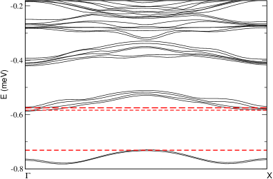
Figure 8: The energy spectrum in the lattice case with $a=8.5\lambda$ (solid lines) compared to lowest energy eigenstates of the isolated vortex (dashed lines). SC parameters correspond to Nb and $z=0.1\lambda$.

Another check on our results is to investigate the dispersion of the lowest-energy bands, in this limit. As discussed before, in the absence of the orbital coupling to the $\vec{A}_{0}$ component of the vector potential, one expects a simple tight-binding dispersion for the lowest bands, with an effective hopping $t$ characterizing the overlap between eigenfunctions trapped under neighboring vortexes. In the presence of the orbital coupling, the hopping matrices pick up an additional phase phase factor proportional to the enclosed flux (the Peierls prescription). This is responsible for lifting the degeneracy of each tight-binding band. The resulting sub-band structure, and in particular the number of sub-gaps opened in each tight-binding band, are known to depend only on the ratio $\phi/\phi_{0}$, where $\phi$ is the flux of the applied magnetic field through the unit cell of the periodic potential. In fact, for $\phi/\phi_{0}=p/q$, where $p$ and $q$ are mutually prime integers, each tight-binding band splits into precisely $q$ subbands Hofstadter (1976). This problem has been well studied as one of the asymptotic limits of the Hofstadter butterfly, corresponding to a large periodic modulation and a small applied magnetic field.

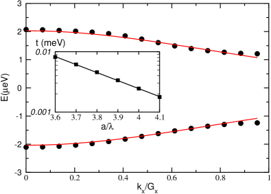
Figure 9: Fit of the energy spectrum of the two lowest energy sub-bands (circles) with the expressions of Eq. (17) appropriate in the asymptotic limit $a\gg\lambda$ (lines). This energy spectrum corresponds $B_{x}=B_{y}=0$ (see text) and $a=4\lambda$, and it is shown as a function of $k_{x}$, with $k_{y}=0$. Its overall energy values have been shifted for convenience. The inset shows the effective hopping $t$ extracted from this fit, which decreases exponentially with increasing distance between vortices.

In our case, $\phi/\phi_{0}=1/2$ and we expect each tight-binding band to split into two sub-bands. This is indeed verified in all the asymptotic limits $a\gg\lambda$ where the tight-binding approximation is appropriate (in some of the plots that we show, such as Fig. 8, this splitting is too small for the lowest band and is not visible on this scale). In fact, we can even fit the dispersion of the bands, in this asymptotic limit. For a triangular lattice with nearest neighbor hopping $t$ (real number), it is straightforward to show that the dispersion when a magnetic field with $\phi/\phi_{0}=1/2$ is added is (see Ref. Hatsugai and Kohmoto, 1990):

$$E(k_{x},k_{y})=\pm 2t\sqrt{1+\cos^{2}(k_{x}a)-\cos(k_{x}a)\cos(k_{y}b)}.$$ (17)

In our case, the hopping $t$ between states trapped under neighboring vortices is not a real number, even if we set $\vec{A}_{0}(\vec{r})=0$ . The reason is that the wave-functions have a non-trivial spinor structure (see Eq. (8)) which leads to a complex value of $t$ ($t$ is just a matrix element related to the overlap of neighboring wavefunctions). To avoid complications coming from dealing with the phase of $t$ and the changes induced by it on the simple dispersion of Eq. (17), we test the fit for a “toy model” in which we set the in-plane magnetic field to zero: $B_{x}(x,y)=B_{y}(x.y)=0$. In this case, the spin is a good quantum number, the ground-state wavefunctions are simple $s$-type waves, the corresponding hopping $t$ is real and Eq. (17) holds. We show a fit for such a case in Fig. 9, along the $k_{y}=0$ line in the Brillouin zone. This fit allows us to extract a value for the effective hopping $t$. As expected (see inset of Fig. 9), $t$ decreases exponentially with increasing distance $a$ between neighboring vortices.

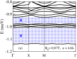
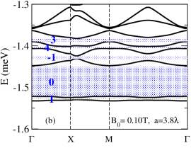
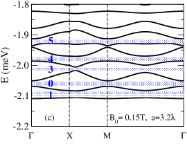
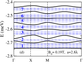
Figure 10: Band structure for the carriers in the DMS QW for $B_{0}$ of (a) $0.07T$;(b) $0.10T$; (a) $0.15T$;(a) $0.19T$. The gaps are marked by shaded regions, and each is labelled with its Chern number (see text).

The presence of the in-plane components changes the structure of the wavefunctions and leads to complex values of $t$, modifying the dispersion from the simple Eq. (17) form. Indeed, as one can see from Fig. 8, the dispersion is now quite different in shape than the one shown for the toy model in Fig. 9. In fact, although there are two distinct subbands $E(k_{x},k_{y})$ for any point in the Brillouin zone, their gaps do not overlap and so there is no true subgap appearing in the band-structure.

These results, corresponding to the asymptotic limit of a large modulation and small applied field, show that our numerical scheme based on expansion in terms of multiple LLs is working well even in this most unfavorable limit. The other asymptotic limit where our results can be easily verified against known predictions is the limit of a large applied field and small periodic modulation. In this case, the small modulation is expected to lift the degeneracy of each LL, but not to lead to mixing amongst the LL. This problem has also been studied extensively Claro and Wannier (1979); Thouless et al. (1982); Pfannkuche and Gerhardts (1992) and the resulting spectrum is also known to depend only on the ratio $\phi/\phi_{0}=p/q$. Unlike in the tight-binding limit, here each LL splits into $p$ subbands.

In our case, $p=1$ and therefore we expect no supplementary structure in the LLs. This is indeed verified, as shown, for example, in Fig. 10 where we plot the evolution of the electronic band structure as $a$ is varied. For $a\gg\lambda$ (panel (a)) we see the emergence of the tight-binding structure discussed above. As $a$ decreases with increasing $B_{0}$ (panel (d)), we indeed see the emergence of nearly equidistant Landau levels, which still exhibit some dispersion due to the weak periodic potential. Because of the large, quasi-uniform Zeeman interaction in this limit, all these states are mostly spin-up and the splitting between consecutive bands corresponds to the cyclotron energy. The intermediary cases (panels (b) and (c)) correspond to situations where neither asymptotic limit is appropriate. In such cases one needs to perform numerical simulations to find the resulting band-structure. The most direct signature of this strongly field-dependent band-structure is obtained in magnetotransport measurements, which we proceed to discuss now.

V Integer Quantum Hall Effect

Following the discovery of the integer quantum Hall effect in a two dimensional electron gas (2DEG) in a strong magnetic field, Laughlin demonstrated that the Hall conductance of a non interacting 2DEG is a multiple of $e^{2}/h$ if the Fermi energy lies in a mobility gap between two LL Laughlin (1981). Later, Thouless et al. argued that the quantization of the Hall conductivity $\sigma_{xy}$ in periodically modulated systems has a topological nature and therefore it occurs whenever the Fermi energy lies in an energy gap, even if the gap lies within a Landau level Thouless et al. (1982). Using the Thouless formula, which we discuss below, the Hall conductances corresponding to various types of lattices, in either of the two asymptotic limits of strong or weak periodic potential, have then been investigated Springsguth et al. (1997).

In our case, it is necessary to use a more general method to calculate the Hall conductance. We briefly review it here. This approach is inspired by the work of KohmotoKohmoto (1985) and Usov Usov (1988), who showed that it is possible to use the topology of the band-structure to calculate, in a relatively simple way, the contribution to the Hall conductance of each filled subband.

When the Fermi level is inside a gap, the total Hall conductivity equals the sum of the contributions from all the fully occupied bands: $\sigma_{xy}=\sum_{\alpha}\sigma_{xy}^{(\alpha)}\Theta(E_{F}-E^{(\alpha)}_{\vec{k}})$. The contribution of each occupied band is Thouless et al. (1982):

$$\sigma^{(\alpha)}_{xy}=i{e^{2}\over 2\pi h}\int d\vec{k}\int d\vec{r}\left[\frac{\partial u_{\vec{k}}^{(\alpha)*}}{\partial k_{x}}\frac{\partial u_{\vec{k}}^{(\alpha)}}{\partial k_{y}}-\frac{\partial u_{\vec{k}}^{(\alpha)*}}{\partial k_{y}}\frac{\partial u_{\vec{k}}^{(\alpha)}}{\partial k_{x}}\right]$$ (18)

where the integrals are carried over the magnetic Brillouin zone and the magnetic unit cell, respectively. Here, $u_{\vec{k}}^{(\alpha)}(\vec{r})=\psi^{(\alpha)}_{\vec{k}}(\vec{r})e^{-i\vec{k}\cdot\vec{r}}$ is the Bloch part of the band eigenstate. Using Eqs. (14) and (15) we can perform the real space integrals explicitly to obtain:

$$\sigma^{(\alpha)}_{xy}={e^{2}\over h}\left[1+{1\over 2\pi}\mbox{Im}\int d\vec{k}\sum_{N\sigma}\frac{\partial d_{N\sigma}^{(\alpha)*}(\vec{k})}{\partial k_{y}}\frac{\partial d_{N\sigma}^{(\alpha)}(\vec{k})}{\partial k_{x}}\right].$$ (19)

The first term is the unit conductance contribution of each LL (band), expected in the absence of the periodic modulation – the usual IQHE. The second term can be rewritten as

$$\Delta\sigma^{(\alpha)}_{xy}={e^{2}\over h2\pi i}\int d\vec{k}\hat{e_{z}}\cdot\left[\nabla_{\vec{k}}\times\vec{A}^{(\alpha)}(\vec{k})\right]$$ (20)

where

$$\vec{A}^{(\alpha)}(\vec{k})=\sum_{N\sigma}d_{N\sigma}^{(\alpha)}(\vec{k})\nabla_{\vec{k}}d_{N\sigma}^{(\alpha)*}(\vec{k}).$$ (21)

This term can be calculated using Kohmoto’s arguments Kohmoto (1985). The magnetic Brillouin zone is a $T^{2}$ torus and has no boundaries. As a result, if the gauge field $\vec{A}^{(\alpha)}(\vec{k})$ is uniquely defined everywhere, Stoke’s theorem shows that this integral vanishes. The gauge field is related to the global phase of the band eigenstates: if $\psi^{(\alpha)}_{\vec{k}}(\vec{r})\rightarrow e^{if(\vec{k})}\psi^{(\alpha)}_{\vec{k}}(\vec{r})$, then $\vec{A}^{(\alpha)}(\vec{k})\rightarrow\vec{A}^{(\alpha)}(\vec{k})-i\nabla_{\vec{k}}f(\vec{k})$. It follows that the gauge field can be uniquely defined if the phase of any one of the components $d_{N\sigma}^{(\alpha)}(\vec{k})$ (and thus, the global phase of the band eigenfunction) can be uniquely defined in the entire magnetic Brillouin zone. This is possible only if the chosen component $d_{N\sigma}^{(\alpha)}(\vec{k})$ has no zeros inside the magnetic Brillouin zone, in which case we can fix the global phase by requesting that this component be real everywhere. In this case, as discussed, $\sigma^{(\alpha)}_{xy}=e^{2}/h$. If there is at least one point $\vec{k}_{0}$ where $d_{N\sigma}^{(\alpha)}(\vec{k}_{0})=0$, in its vicinity the global phase must be defined from the condition that some other component $d_{N^{\prime}\sigma^{\prime}}^{(\alpha)}(\vec{k})$, which is finite in this region, is real. The definitions of the global phase inside and outside this vicinity of $\vec{k}_{0}$ are related through a gauge transformation; moreover, the torus now has a boundary separating the two areas. Applying Stokes’ theorem, it follows immediately Kohmoto (1985) that $\Delta\sigma^{(\alpha)}_{xy}={e^{2}\over h}S_{0}$. The integer $S_{0}$ is the winding number in the phase of $d_{N^{\prime}\sigma^{\prime}}^{(\alpha)}(\vec{k})$ (when $d_{N\sigma}^{(\alpha)}(\vec{k})$ is real) on any contour surrounding $\vec{k}_{0}$. If $d_{N\sigma}^{(\alpha)}(\vec{k})$ has several zeros inside the Brillouin zone, then one has to sum the winding numbers associated with each zero:

$$\sigma^{(\alpha)}_{xy}=\frac{e^{2}}{h}\left[1+\sum_{m}S_{m}\right]$$ (22)

Thus, once the coefficients $d_{N\sigma}^{(\alpha)}(\vec{k})$ are known, one can immediately find the contribution of the band $\alpha$ to $\sigma_{xy}$ by studying their zeros and their vorticities.

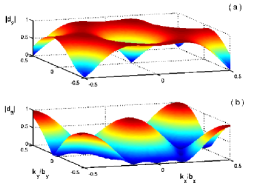
Figure 11: Values in the magnetic Brillouin zone of the $d^{(\alpha)}_{N,\sigma}(\vec{k})$ coefficients corresponding to the second band $\alpha=2$, in the band-structure obtained for $B_{0}=0.095T$, $z=8$ nm and $g=500$. a) $d^{(2)}_{2,\uparrow}(\vec{k})$ is chosen to be real everuwhere. It has zeros in the corners and center of the magnetic Brillouin zone. b) $|d^{(2)}_{3,\uparrow}(\vec{k})|$ has maxima where $d^{(2)}_{2,\uparrow}(\vec{k})$ has zeroes.

As an illustration of this method, we calculate the contribution of the second band $\alpha=2$, for $B_{0}=0.095T$, $z=8$ nm and $g=500$. We first choose the overall phasefactor for the corresponding coefficients $d^{(2)}_{N,\sigma}(\vec{k})$ defining this band so that one of them (specifically, here we chose $N=2$) is real throughout the Brillouin zone, see Fig. 11. We see that this component has zeros in some high-symmetry points, signalling a potentially non-trivial contribution to $\sigma_{xy}$. In order to find the corresponding vorticities, we investigate any other component that has no zeros at the positions of the singular points of $d^{(2)}_{2,\uparrow}$. In general, this other component will have complex values. In the lower panel of Fig. 11 we plot the absolute value of $d^{(2)}_{3,\uparrow}$, which is indeed finite at all zeros of $d^{(2)}_{2,\uparrow}$.

The vorticities can be found by investigating the variation in the phase of $d^{(2)}_{3,\uparrow}$ around the zeros of $d^{(2)}_{2,\uparrow}$. The phase-map of $d^{(2)}_{3,\uparrow}$ is shown in Fig. (12), where red represents a phase of $\pi$ and blue a phase of $-\pi$. Any boundary red-blue indicated a non-zero winding number. These winding numbers $S_{m}$ (in units of 2$\pi$) are the phase incursions of $d^{(2)}_{3,\uparrow}$ upon going anticlockwise around the singular points. In this case, it is clear that the phase incursions are of $-2\pi$. As there are two singular points in the MBZ (the corners count as 1/4 each), the conductance of the subband 2 is $\sigma^{(2)}_{xy}=(\frac{e^{2}}{h})(1-2)=-(\frac{e^{2}}{h})$. The same overall value is obtained by looking at the vorticities of any other wavefunction that is finite at the zeros of $d^{(2)}_{2,\uparrow}$.

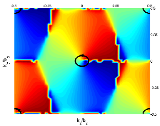
Figure 12: Phase map of $d^{(2)}_{3,\uparrow}$ inside the MBZ. Blue represents $-\pi$ and red represents $\pi$. The phase winds by $-2\pi$ around both the center and the corner points.

Larger winding numbers are also possible. As a second example, in Fig. 13 we show the phase map for the component $d^{(6)}_{8,\uparrow}$ for the sixth band. In this case, we requested that the component $d^{(6)}_{6\uparrow}$ be real, and we found its zeros to be again in the center and corners of the Brillouin zone. Now, the phase incursion about the zeros are $-2\times 2\pi$ and therefore the conductance of the 6^th subband is, in this case, $\sigma^{(6)}_{xy}=(\frac{e^{2}}{h})(1-4)=-3(\frac{e^{2}}{h})$. These integers are called Chern numbers.

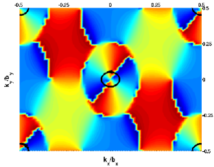
Figure 13: Same as in Fig. 12 but for component $d^{(6)}_{8,\uparrow}(\vec{k})$.

As discussed by Avron et al. Avron et al. (1983), based on the topological nature of the Hall conductance it can be shown that the Chern number of a subband does not change unless the subband merges with a neighboring subband. In this case, the Chern number of the newly formed band equals the sum of the Chern numbers of the two subbands. Similarly, if a band splits into one or more subbands, its Chern number is re-distributed over the two or more subbands. In the system discussed here, a variation of the applied magnetic field $B_{0}$ changes the band structure, opening and closing energy gaps. By calculating the energy spectrum of the system for a given range of the magnetic field, we map the opening and closing of the gaps between the few lowest mini-bands as a function of $B_{0}$ (see Fig. 10). We than calculate the Hall conductance of each of the lowest seven mini-band for each configuration of gaps using this method.

It is important to point out that we recover the expected values of the Hall conductance of the minibands in both limits of strong and weak modulation for a triangular lattice and $p/q=1/2$. In Fig. 10, we see in panel (b) that the first two jumps in the conductivity are $1e^{2}/h$ and then $-1e^{2}/h$, as expected for the $p=2$ subbands of tight-binding limit of the triangular Hofstadter butterfly Hatsugai and Kohmoto (1990). In the limit of weak modulation, we obtain the usual IQHE, as expected, since $p=1$.

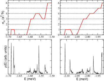
Figure 14: Density of states and hall conductivity as a function of the Fermi Energy for two different applied magnetic fields B₀.

Such a calculation allows us to predict the sequence of plateaus in the IQHE if one keeps $B_{0}$ fixed and varies the concentration of electrons in the DMS (for instance, by varying the value of a back-gate voltage). Such predictions are shown in Fig. 14, where we plot the density of states (lower panels) and the corresponding Hall conductivity (upper panels) as a function of the Fermi energy for band-structure corresponding to two different values of $B_{0}$. Of course, one needs disorder in order to observe the IQHE. We did not include disorder in this calculation, but we know from Laughlin’s arguments that the value of the Chern numbers remains the same, in its presence. The plots in the upper pannels of Fig. 14 are thus only sketches of the expected Hall conductances, in these cases. The main observation is that the Hall conductivity does not increase monotonically as a function of $E_{F}$, as is the case in the usual IQHE. This, of course, is due to the presence of the periodic potential induced by the vortex lattice, and clearly signals the formation of the Hofstadter butterfly.

We can summarize more efficiently the information shown in plots like Fig. 14 in the following way. The two important parameters are the values of the electron concentration when the Fermi level is in a gap, and the value of $\sigma_{xy}$ expected for that gap. Such a plot is shown in Fig. 15. The various colored regions are centered on the values of the electron concentrations where the Fermi energy should be in a gap. These regions are assigned an arbitrary width (calculations involving realistic disorder are needed to find the widths of these plateaus) and are labelled with the integer $i$ defining the quantized value of $\sigma_{xy}=i(e^{2}/h)$. As the external magnetic field is varied, some subbands merge and then separate, changing their individual Chern numbers in the process. This plot allows us to predict the sequence of Hall plateaus for a constant value of the electron density $n$ and varying external field, as shown in the inset for $n=5.5\times 10^{10}$ cm^-2. The non-monotonic sequences of plateaus as $B_{0}$ decreases clearly signals the appearance of tight-binding bands, which in turn show that the Zeeman potential is strong enough to localize spin-polarized charge carries under individual vortices.

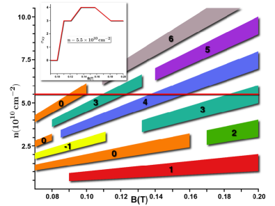
Figure 15: conductivity $\sigma_{xy}$ in units of $e^{2}/h$, as a function of the magnetic field $B$ and the charge carrier density $n$. The colored areas mark the gaps between the bands. For some ranges of $B$, neighboring bands touch and some of the gaps close. The integers give the quantized values of the $\sigma_{xy}$ plateaus. For example, $\sigma_{xy}$ as a function of $B$, at a constant density n$=5.5\times 10^{10}$cm^-2 (red line) is shown in the inset. It is quantized every time the Fermi level is inside a gap. The parameters are the same as for Fig. 6.

VI Concluding remarks

In this paper we presented detailed numerical and analytical calculations aimed at investigating the novel spin and charge properties of a magnetic semiconductor quantum well in close proximity of a superconducting flux line lattice. First we have shown how the single superconducting vortex localizes spin polarized states, with binding energies within the accessible range of several local spectroscopic probes, as well as transport measurements. We then turned our attention to the case of a periodic flux line lattice, and presented the results of a numerical framework able to interpolate between the inhomogeneous (low) field regime of dilute vortex lattice and the homogeneous (high) field regime characterized by Landau level quantization. Our numerical scheme not only reproduces the energy spectrum of the isolated vortex limit, but the spin-polarized electronic band structure we obtain within this framework also matches with the analytical tight binding calculations applied for the dilute vortex lattice limit as well. Between the two extreme field limits we investigated the momentum-space topology of the Bloch wave functions associated with the spin polarized bands. By using the connection between the wave function topology and quantum Hall conductance, we showed how the consequences of the 1/2 Hofstadter butterfly spectrum can lead to experimentally observable effects, such as a non-monotonic ’staircase’ of Hall plateaus as they appear under a varying magnetic field or carrier concentration. We paid special attention to provide realistic systems and materials parameters for each experimental configuration we suggested. All indications from our theory seem to suggest that the magnetic semiconductor-superconductor hybrids can be fabricated with presently available molecular-beam epitaxy will provide us with a rich variety of transport and spectroscopic phenomena.

VII Acknowledgements

We would like to thank A. Abrikosov, J.K. Furdyna, T. Wojtowicz, P. Redlinski, G. Mihaly, and G. Zarand for useful discussions. T.G.R. acknowledges partial financial support by Brazilian agencies CNPq (research grant 55.6552/2005-9) and Instituto do Milênio para Nanociência. B.J. was supported by NSF-NIRT award DMR02-10519 and the Alfred P. Sloan Foundation.

References

- Ohno (1996) H. Ohno, Applied Physics Letters 69, 262 (1996).
- Furdyna (1988) J. K. Furdyna, Journal Of Applied Physics 64, R29 (1988).
- Lee (2000) S. Lee, Physical Review B 61, 2120 (2000).
- Fiederling et al. (1999) R. Fiederling, M. Keim, G. Reuscher, W. Ossau, G. Schmidt, A. Waag, and L. W. Molenkamp, Nature 402, 787 (1999).
- Berciu and Janko (2003) M. Berciu and B. Janko, Physical Review Letters 90, 246804 (2003).
- Redlinski et al. (2005a) P. Redlinski, T. G. Rappoport, A. Libal, J. K. Furdyna, B. Janko, and T. Wojtowicz, Applied Physics Letters 86, 113103 (2005a).
- Redlinski et al. (2005b) P. Redlinski, T. Wojtowicz, T. G. Rappoport, A. Libal, J. K. Furdyna, and B. Janko, Physical Review B 72, 085209 (2005b).
- Berciu et al. (2005) M. Berciu, T. G. Rappoport, and B. Janko, Nature 435, 71 (2005).
- Peeters and Matulis (1993) F. M. Peeters and A. Matulis, Physical Review B 48, 15166 (1993).
- Freire et al. (2000) J. A. K. Freire, A. Matulis, F. M. Peeters, V. N. Freire, and G. A. Farias, Physical Review B 61, 2895 (2000).
- Rammer and Shelankov (1987) J. Rammer and A. L. Shelankov, Physical Review B 36, 3135 (1987).
- Brey and Fertig (1993) L. Brey and H. A. Fertig, Physical Review B 47, 15961 (1993).
- Chang and Niu (1994) M. C. Chang and Q. Niu, Physical Review B 50, 10843 (1994).
- Nielsen and Hedegrd (1995) M. Nielsen and P. Hedegrd, Physical Review B 51, 7679 (1995).
- Gumbs et al. (1995) G. Gumbs, D. Miessein, and D. Huang, Physical Review B 52, 14755 (1995).
- Oh (1999) G.-Y. Oh, Physical Review B 60, 1939 (1999).
- Matulis and Peeters (2000) A. Matulis and F. M. Peeters, Physical Review B (Condensed Matter and Materials Physics) 62, 91 (2000).
- Wang et al. (2004) X. F. Wang, P. Vasilopoulos, and F. M. Peeters, Physical Review B 70, 155312 (2004).
- Bending et al. (1990) S. J. Bending, K. Vonklitzing, and K. Ploog, Physical Review Letters 65, 1060 (1990).
- Geim et al. (1992) A. K. Geim, S. J. Bending, and I. V. Grigorieva, Physical Review Letters 69, 2252 (1992).
- Danckwerts et al. (2000) M. Danckwerts, A. R. Goni, C. Thomsen, K. Eberl, and A. G. Rojo, Physical Review Letters 84, 3702 (2000).
- Claro and Wannier (1979) F. H. Claro and G. H. Wannier, Physical Review B 19, 6068 (1979).
- Hofstadter (1976) D. R. Hofstadter, Physical Review B 14, 2239 (1976).
- Schlosser et al. (1996) T. Schlosser, K. Ensslin, J. P. Kotthaus, and M. Holland, Europhysics Letters 33, 683 (1996).
- Albrecht et al. (2001) C. Albrecht, J. H. Smet, K. von Klitzing, D. Weiss, V. Umansky, and H. Schweizer, Physical Review Letters 86, 147 (2001).
- Melinte et al. (2004) S. Melinte, M. Berciu, C. Zhou, E. Tutuc, S. J. Papadakis, C. Harrison, E. P. De Poortere, M. Wu, P. M. Chaikin, M. Shayegan, et al., Physical Review Letters 92, 036802 (2004).
- Pearl (1964) J. Pearl, Applied Physics Letters 5, 65 (1964).
- Kirtley et al. (1999) J. R. Kirtley, V. G. Kogan, J. R. Clem, and K. A. Moler, Physical Review B 59, 4343 (1999).
- Carneiro and Brandt (2000) G. Carneiro and E. H. Brandt, Physical Review B 61, 6370 (2000).
- Brandt (1995) E. H. Brandt, Reports On Progress In Physics 58, 1465 (1995).
- Bhattacharya and Higgins (1993) S. Bhattacharya and M. J. Higgins, Physical Review Letters 70, 2617 (1993).
- Bugoslavsky et al. (2001) Y. Bugoslavsky, G. K. Perkins, X. Qi, L. F. Cohen, and A. D. Caplin, Nature 410, 563 (2001).
- Yamamoto et al. (1994) H. Yamamoto, K. Yoshii, K. Saiki, and A. Koma, Journal of Vacuum Science and Technology A: Vacuum, Surfaces, and Films 12, 125 (1994).
- Abrikosov (1957) A. A. Abrikosov, Soviet Physics JETP 5, 1174 (1957).
- Zak (1964) J. Zak, Physical Review 136, A776 (1964).
- Thouless et al. (1982) D. J. Thouless, M. Kohmoto, M. P. Nightingale, and M. Dennijs, Physical Review Letters 49, 405 (1982).
- Pfannkuche and Gerhardts (1992) D. Pfannkuche and R. R. Gerhardts, Physical Review B 46, 12606 (1992).
- Demikhovskii and Khomitsky (2003) V. Y. Demikhovskii and D. V. Khomitsky, Physical Review B 67 (2003).
- Usov (1988) N. A. Usov, Soviet Physics JETP 67, 2565 (1988).
- Hatsugai and Kohmoto (1990) Y. Hatsugai and M. Kohmoto, Physical Review B 42, 8282 (1990).
- Laughlin (1981) R. B. Laughlin, Physical Review B 23, 5632 (1981).
- Springsguth et al. (1997) D. Springsguth, R. Ketzmerick, and T. Geisel, Physical Review B 56, 2036 (1997).
- Kohmoto (1985) M. Kohmoto, Annals Of Physics 160, 343 (1985).
- Avron et al. (1983) J. E. Avron, R. Seiler, and B. Simon, Physical Review Letters 51, 51 (1983).