First-Principles Perturbative Computation of Phonon Properties of Insulators
in Finite Electric Fields

Abstract

We present a perturbative method for calculating phonon properties of an insulator in the presence of a finite electric field. The starting point is a variational total-energy functional with a field-coupling term that represents the effect of the electric field. This total-energy functional is expanded in small atomic displacements within the framework of density-functional perturbation theory. The linear response of field-polarized Bloch functions to atomic displacements is obtained by minimizing the second-order derivatives of the total-energy functional. In the general case of nonzero phonon wavevector, there is a subtle interplay between the couplings between neighboring k-points introduced by the presence of the electric field in the reference state, and further-neighbor k-point couplings determined by the wavevector of the phonon perturbation. As a result, terms arise in the perturbation expansion that take the form of four-sided loops in k-space. We implement the method in the ABINIT code and perform illustrative calculations of the field-dependent phonon frequencies for III-V semiconductors.

I Introduction

The understanding of ferroelectric and piezoelectric materials, whose physics is dominated by soft phonon modes, has benefited greatly from the availability of first-principles methods for calculating phonon properties. In general, these methods can be classified into two main types, the direct or frozen-phonon approachdirect1 ; direct2 and the linear-response approach.dfpt3 ; dfpt2 In the former approach, the properties of phonons at commensurate wavevectors are obtained from supercell calculations of forces or total-energy changes between between equilibrium and distorted structures. In the latter approach, based on density-functional perturbation theory (DFPT), expressions are derived for the second derivatives of the total energy with respect to atomic displacements, and these are calculated by solving a Sternheimer equationdfpt3 or by using minimization methods.dfpt2 ; dfpt1 Compared to the direct approach, the linear-response approach has important advantages in that time-consuming supercell calculations are avoided and phonons of arbitrary wavevector can be treated with a cost that is independent of wavevector. However, existing linear-response methods work only at zero electric field.

The development of first-principles methods for treating the effect of an electric field ${\cal E}$ in a periodic system has been impeded by the presence of the electrostatic potential ${\cal E}\cdot{\bf r}$ in the Hamiltonian. This potential is linear in real space and unbounded from below, and thus is incompatible with periodic boundary conditions. The electronic bandstructure becomes ill-defined after application of a potential of this kind. Many attempts have been made to overcome this difficulty. For example, linear-response approaches have been used to treat the electric field as a perturbation.dfpt1 ; baroni01 It is possible to formulate these approaches so that only the off-diagonal elements of the position operator, which remain well defined, are needed, thus allowing for the calculation of Born effective charges, dielectric constants, etc. Since it is a perturbative approach, a finite electric field cannot be introduced.

Recently, a total-energy method for treating insulators in nonzero electric fields has been proposed.souza02 ; umari02 In this approach, an electric enthalpy functional is defined as a sum of the usual Kohn-Sham energy and an ${\cal E}\cdot{\bf P}$ term expressing the linear coupling of the electric field to the polarization $\bf P$. The enthalpy functional is minimized with respect to field-polarized Bloch states, and the information on the response to the electric field is contained in these optimized Bloch states. Using this approach, it is possible to carry out calculations of dynamical effective charges, dielectric susceptibilities, piezoelectric constants, etc., using finite-difference methods.souza02 ; umari02 It would also be possible to use it to study phonon properties in finite electric field, but with the aforementioned limitations (large supercells, commensurate wavevectors) of the direct approach.

In this work, we build upon these recent developments by showing how to extend the linear-response methods so that they can be applied to the finite-field case. That is, we formulate DFPT for the case in which the unperturbed system is an insulator in a finite electric field. Focusing on the case of phonon perturbations, we derive a tractable computational scheme and demonstrate its effectiveness by carrying out calculations of phonon properties of polar semiconductors in finite electric fields.

This paper is organized as follows. In Sec. II we review the total-energy functional appropriate for describing an insulator in an electric field, and discuss the effect of the electric field on the phonon frequencies both for our exact theory and for a previous approximate theory. The second-order expansion of the total-energy functional is derived in Sec. III, and expressions for the force-constant matrix are given, first for phonons at the Brillouin zone center and then for arbitrary phonons. In Sec. IV we report some test calculations of field-induced changes of phonon frequencies in the III-V semiconductors GaAs and AlAs. Section V contains a brief summary and conclusion.

II Background and definitions

II.1 Electrical enthalpy functional

We start from the electric enthalpy functional souza02

$$F[{\bf R};\psi;{\cal E}]=E_{\rm KS}[{\bf R};\psi]-\Omega{\cal E}\cdot{\bf P}_{\rm mac}[\psi],$$ (1)

where $E_{\rm KS}$ has the same form as the usual Kohn-Sham energy functional in the absence of an electric field. Here $\Omega$ is the cell volume, ${\bf P}_{\rm mac}$ is the macroscopic polarization, ${\cal E}$ is the homogeneous electric field, ${\bf R}$ are the atomic positions, and $\psi$ are the field-polarized Bloch functions. Note that ${\bf P}_{\rm mac}$ has both ionic and electronic contributions. The former is an explicit function of ${\bf R}$, while the latter is an implicit function of ${\bf R}$ through the Bloch functions, which also depend on the atomic positions. When an electric field is present, a local minimum of this functional describes a long-lived metastable state of the system rather than a true ground state (indeed, a true ground state does not exist in finite electric field).souza02

According to the modern theory of polarization,smith93 the electronic contribution to the macroscopic polarization is given by

$${\bf P}_{\rm mac}=\frac{ief}{(2\pi)^{3}}\sum_{n=1}^{M}\int_{\rm BZ}d{\bf k}\langle u_{{\bf k}n}|\nabla_{k}|u_{{\bf k}n}\rangle,$$ (2)

where $e$ is the charge of an electron ($e<0$), $f$=2 for spin degeneracy, $M$ is the number of occupied bands, $u_{{\bf k}n}$ are the cell-periodic Bloch functions, and the integral is over the Brillouin zone (BZ). Making the transition to a discretized k-point mesh, this can be written in a form

$${\bf P}_{\rm mac}=\frac{ef}{2\pi\Omega}\sum_{i=1}^{3}\frac{{\bf a}_{i}}{N_{\perp}^{(i)}}\sum_{l=1}^{N_{\perp}^{(i)}}\textrm{Im}\ln\prod_{j=1}^{N_{i}}\det S_{{\bf k}_{lj},{\bf k}_{l,j+1}}$$ (3)

that is amenable to practical calculations. In this expression, for each lattice direction $i$ associated with primitive lattice vector ${\bf a}_{i}$, the BZ is sampled by $N_{\perp}^{(i)}$ strings of k-points, each with $N_{i}$ points spanning along the reciprocal lattice vector conjugate to ${\bf a}_{i}$, and

$$(S_{{\bf k}{\bf k}^{\prime}})_{mn}=\langle u_{m{\bf k}}|u_{n{\bf k}^{\prime}}\rangle$$ (4)

are the overlap matrices between cell-periodic Bloch vectors at neighboring locations along the string. Because Eqs. (2-3) can be expressed in terms of Berry phases, this is sometimes referred to as the “Berry-phase theory” of polarization.

II.2 Effect of electric field on phonon frequencies

II.2.1 Exact theory

We work in the framework of a classical zero-temperature theory of lattice dynamics, so that quantum zero-point and thermal anharmonic effects are neglected. In this context, the phonon frequencies of a crystalline insulator depend upon an applied electric field in three ways: (i) via the variation of the equilibrium lattice vectors (i.e., strain) with applied field; (ii) via the changes in the equilibrium atomic coordinates, even at fixed strain; and (iii) via the changes in the electronic wavefunctions, even at fixed atomic coordinates and strain. Effects of type (i) (essentially, piezoelectric and electrostrictive effects) are beyond the scope of the present work, but are relatively easy to include if needed. This can be done by computing the relaxed strain state as a function of electric field using the approach of Ref. souza02, , and then computing the phonon frequencies in finite electric field for these relaxed structures using the methods given here. Therefore, in the remainder of the paper, the lattice vectors are assumed to be independent of electric field unless otherwise stated, and we will focus on effects of type (ii) (“lattice effects”) and type (iii) (“electronic effects”).

In order to separate these two types of effects, we first write the change in phonon frequency resulting from the application of the electric field as

$$\Delta\omega({\bf q};{\cal E})=\omega({\bf q};{\bf R}_{\cal E},{\cal E})-\omega({\bf q};{\bf R}_{0},0),$$ (5)

where $\omega({\bf q};{\bf R},{\cal E})$ is the phonon frequency extracted from the second derivative of the total energy of Eq. (1) with respect to the phonon amplitude of the mode of wavevector ${\bf q}$, evaluated at displaced coordinated $\bf R$ and with electrons experiencing electric field ${\cal E}$. Also, ${\bf R}_{\cal E}$ are the relaxed atomic coordinates at electric field ${\cal E}$, while ${\bf R}_{0}$ are the relaxed atomic coordinates at zero electric field. Then Eq. (5) can be decomposed as

$$\Delta\omega({\bf q};{\cal E})=\Delta\omega_{\rm el}({\bf q};{\cal E})+\Delta\omega_{\rm ion}({\bf q};{\cal E})$$ (6)

where the electronic part of the response is defined to be

$$\Delta\omega_{\rm el}({\bf q};{\cal E})=\omega({{\bf q};\bf R}_{0},{\cal E})-\omega({\bf q};{\bf R}_{0},0)$$ (7)

and the lattice (or “ionic”) part of the response is defined to be

$$\Delta\omega_{\rm ion}({\bf q};{\cal E})=\omega({\bf q};{\bf R}_{\cal E},{\cal E})-\omega({\bf q};{\bf R}_{0},{\cal E}).$$ (8)

In other words, the electronic contribution reflects the influence of the electric field on the wavefunctions, and thereby on the force-constant matrix, but evaluated at the zero-field equilibrium coordinates. By contrast, the ionic contribution reflects the additional frequency shift that results from the field-induced ionic displacements.

The finite-electric-field approach of Refs. souza02, -umari02, provides the methodology needed to compute the relaxed coordinates ${\bf R}_{\cal E}$, and the electronic states, at finite electric field ${\cal E}$. The remainder of this work is devoted to developing and testing the techniques for computing $\omega({\bf q};{\bf R},{\cal E})$ for given ${\bf q}$, $\rm R$, and ${\cal E}$, needed for the evaluation of Eq. (5). We shall also use these methods to calculate the various quantities needed to perform the decomposition of Eqs. (6-8), so that we can also present results for $\Delta\omega_{\rm el}$ and $\Delta\omega_{\rm ion}$ separately in Sec. IV.

II.2.2 Approximate theory

Our approach above is essentially an exact one, in which Eq. (5) is evaluated by computing all needed quantities at finite electric field. However, we will also compare our approach with an approximate scheme that has been developed in the literature over the last few years,sai02 ; fu03 ; naumov05 ; antons05 in which the electronic contribution is neglected and the lattice contribution is approximated in such a way that the finite-electric-field approach of Refs. souza02, -umari02, is not needed.

This approximate theory can be formulated by starting with the approximate electric enthalpy functionalsai02

$$F[{\bf R};{\cal E}]=E^{(0)}_{\rm KS}[{\bf R}]-\Omega{\cal E}\cdot{\bf P}_{\rm mac}^{(0)}[{\bf R}],$$ (9)

where $E^{(0)}_{\rm KS}[{\bf R}]$ is the zero-field ground-state Kohn-Sham energy at coordinates $\bf R$, and ${\bf P}_{\rm mac}^{(0)}$ is the corresponding zero-field electronic polarization. In the presence of an applied electric field ${\cal E}$, the equilibrium coordinates that minimize Eq. (9) satisfy the force-balance equation

$$-\frac{dE^{(0)}_{\rm KS}}{d{\bf R}}+{\bf Z}^{(0)}\cdot{\cal E}=0$$ (10)

where ${\bf Z}^{(0)}=\Omega\,d{\bf P}_{\rm mac}^{(0)}/d{\bf R}$ is the zero-field dynamical effective charge tensor. That is, the sole effect of the electric field is to make an extra contribution to the atomic forces that determine the relaxed displacements; the electrons themselves do not “feel” the electric field except indirectly through these displacements. In Ref. sai02, , it was shown that this theory amounts to treating the coupling of the electric field to the electronic degrees of freedom in linear order only, while treating the coupling to the lattice degrees of freedom to all orders. Such a theory has been shown to give good accuracy in cases where the polarization is dominated by soft polar phonon modes, but not in systems in which the electronic and lattice polarizations are comparable.sai02 ; fu03 ; naumov05 ; antons05 ; dieguez06

In this approximate theory, the effect of the electric field on the lattice dielectric propertiesantons05 and phonon frequenciesnaumov05 comes about through the field-induced atomic displacements. Thus, in the notation of Eqs. (5-8), the frequency shift (relative to zero field) is

$$\Delta\omega_{\rm ion}^{\prime}({\bf q};{\cal E})=\omega({\bf q};{\bf R}^{\prime}_{\cal E},0)-\omega({\bf q};{\bf R}_{0},0)$$ (11)

in this approximation, where ${\bf R}^{\prime}_{\cal E}$ is the equilibrium position according to Eq. (10). We will make comparisons between the exact ${\bf R}_{\cal E}$ and the approximate ${\bf R}^{\prime}_{\cal E}$, and the corresponding frequency shifts $\Delta\omega_{\rm ion}({\bf q},{\cal E})$ and $\Delta\omega_{\rm ion}^{\prime}({\bf q},{\cal E})$ later in Sec. IV.

III Perturbation expansion of the electric enthalpy functional

We consider an expansion of the properties of the system in terms of small displacements $\lambda$ of the atoms away from their equilibrium positions, resulting in changes in the charge density, wavefunctions, total energy, etc. We will be more precise about the definition of $\lambda$ shortly. We adopt a notation in which the perturbed physical quantities are expanded in powers of $\lambda$ as

$$Q(\lambda)=Q^{(0)}+\lambda Q^{(1)}+\lambda^{2}Q^{(2)}+\lambda^{3}Q^{(3)}+...$$ (12)

where $Q^{(n)}=(1/n!)d^{n}Q/d\lambda^{n}$. The immediate dependence upon atomic coordinates is through the external potential $v_{{\rm ext}}(\lambda)$, which has no electric-field dependence and thus depends upon coordinates and pseudopotentials in the same way as in the zero-field case. The changes in electronic wavefunctions, charge density, etc. can then be regarded as being induced by the changes in $v_{{\rm ext}}$.

III.1 Zero q wavevector case

The nuclear positions can be expressed as

$${\bf R}_{n\nu}={\bf t}_{n}+{\bf d}_{\nu}+{\bf b}_{n\nu},$$ (13)

where ${\bf t}_{n}$ is a lattice vector, ${\bf d}_{\nu}$ is a basis vector within the unit cell, and ${\bf b}_{n\nu}$ is the instantaneous displacement of atom $\nu$ in cell $n$. We consider in this section a phonon of wavevector ${\bf q}={\bf 0}$, so that the perturbation does not change the periodicity of the crystal, and the perturbed wavefunctions satisfy the same periodic boundary condition as the unperturbed ones. To be more precise, we choose one sublattice $\nu$ and one Cartesian direction $\alpha$ and let $b_{n\nu\alpha}=\lambda$ (independent of $n$), so that we are effectively moving one sublattice in one direction while while freezing all other sublattice displacements. Since the electric enthalpy functional of Eq. (1) is variational with respect to the field-polarized Bloch functions under the constraints of orthonormality, a constrained variational principle exists for the second-order derivative of this functional with respect to atomic displacements.gonze95 In particular, the correct first-order perturbed wavefunctions $\psi^{(1)}_{m{\bf k}}$ can be obtained by minimizing the second-order expansion of the total energy with respect to atomic displacements,

$$F^{(2)}[\psi_{m{\bf k}}^{(0)};{\cal E}] = \min_{\psi^{(1)}}\bigg{(}E_{\rm KS}[\psi^{(0)}_{m{\bf k}};\psi^{(1)}_{m{\bf k}}]$$ (14)

$$-\Omega{\bf P}_{\rm mac}[\psi^{(0)}_{m{\bf k}};\psi^{(1)}_{m{\bf k}}]\cdot{\cal E}\bigg{)}^{(2)},$$

subject to the constraints

$$\langle\psi_{m{\bf k}}^{(0)}|\psi_{n{\bf k}}^{(1)}\rangle=0$$ (15)

(where $m$ and $n$ run over occupied states). The fact that only zero-order and first-order wavefunctions appear in Eq. (14) is a consequence of the “2$n$+1 theorem.”gonze95

Recalling that $|\psi_{n{\bf k}}^{(1)}\rangle$ is the first-order wavefunction response to a small real displacement $\lambda$ of basis atom ${\nu}$ along Cartesian direction $\alpha$, we can expand the external potential as

$$v_{{\rm ext}}({\bf r})=v_{{\rm ext}}^{(0)}({\bf r})+v^{(1)}_{{\rm ext},\nu\alpha}({\bf r})\lambda+v^{(2)}_{{\rm ext},\nu\alpha}({\bf r})\lambda^{2}+...$$ (16)

where

$$v^{(1)}_{\rm ext,\nu\alpha}({\bf r})=\sum_{n}\frac{\partial v_{\rm ext}({\bf r})}{\partial R_{n\nu\alpha}}\;,$$ (17)

$$v^{(2)}_{\rm ext,\nu\alpha}({\bf r})=\sum_{n}\frac{\partial^{2}v_{\rm ext}({\bf r})}{\partial R_{n\nu\alpha}^{2}}\;,$$ (18)

etc. From this we shall construct the second-order energy $F^{(2)}$ of Eq. (14), which has to be minimized in order to find $|\psi_{n{\bf k}}^{(1)}\rangle$. The minimized value of $F^{(2)}$ gives, as a byproduct, the diagonal element of the force-constant matrix associated with displacement $\nu\alpha$. Once the $|\psi_{n{\bf k}}^{(1)}\rangle$ have been computed for all $\nu\alpha$, the off-diagonal elements of the force-constant matrix can be calculated using a version of the $2n+1$ theorem as will be described in Sec. III.1.3.

III.1.1 Discretized k mesh

In practice, we always work on a discretized mesh of k-points, and we have to take into account the orthogonality constraints among wavefunctions at a given k-point on the mesh. Here, we are following the “perturbation expansion after discretization” (PEAD) approach introduced in Ref. nunes01, . That is, we write down the energy functional in its discretized form, and then consistently derive perturbation theory from this energy functional. Introducing Lagrange multipliers $\Lambda_{{\bf k},mn}$ to enforce the orthonormality constraints

$$\langle\psi_{m{\bf k}}|\psi_{n{\bf k}}\rangle=\delta_{mn},$$ (19)

where $\psi_{n{\bf k}}$ are the Bloch wavefunctions, and letting $N$ be the number of k-points, the effective total-energy functional of Eq. (1) can be written as

$$F=F_{\rm KS}+F_{\rm BP}+F_{\rm LM}$$ (20)

where $F_{\rm KS}=E_{\rm KS}$, $F_{\rm BP}=-\Omega{\bf P}_{\rm mac}\cdot{\cal E}$, and $F_{\rm LM}$ are the Kohn-Sham, Berry-phase, and Lagrange-multiplier terms, respectively. The first and last of these are given by

$$F_{\rm KS}=\frac{f}{N}\sum_{{\bf k}n}^{\rm occ}\langle\psi_{n{\bf k}}|T+v_{{\rm ext}}|\psi_{n{\bf k}}\rangle+E_{\rm Hxc}[n],$$ (21)

and

$$F_{\rm LM}=-\frac{f}{N}\sum_{{\bf k},mn}^{\rm occ}\Lambda_{{\bf k},mn}(\langle\psi_{m{\bf k}}|\psi_{n{\bf k}}\rangle-\delta_{mn}),$$ (22)

where $N$ is the number of k-points in the BZ. As for the Berry-phase term, we modify the notation of Eq. (3) slightly to write this as

$$F_{\rm BP}=-\frac{ef}{2\pi}\sum_{i=1}^{3}\frac{{\cal E}\cdot{\bf a}_{i}}{N_{\perp}^{(i)}}\sum_{{\bf k}}D_{{\bf k},{\bf k}+{\bf g}_{i}}$$ (23)

where

$$D_{{\bf k}{\bf k}^{\prime}}=\textrm{Im}\ln\det S_{{\bf k}{\bf k}^{\prime}}$$ (24)

and ${\bf g}_{i}$ is the reciprocal lattice mesh vector in lattice direction $i$. (That is, ${\bf k}$ and ${\bf k}+{\bf g}_{i}$ are neighboring k-points in one of the $N_{\perp}^{(i)}$ strings of k-points running in the reciprocal lattice direction conjugate to ${\bf a}_{i}$.) Recall that the matrix of Bloch overlaps was defined in Eq. (4).

We now expand all quantities in orders of the perturbation, e.g., $\Lambda(\lambda)=\Lambda^{(0)}+\lambda\Lambda^{(1)}+\lambda^{2}\Lambda^{(2)}+...$, etc. Similarly, we expand $S_{{\bf k}{\bf k}^{\prime}}(\lambda)=S_{{\bf k}{\bf k}^{\prime}}^{(0)}+\lambda S_{{\bf k}{\bf k}^{\prime}}^{(1)}+\lambda^{2}S_{{\bf k}{\bf k}^{\prime}}^{(2)}+...$, and we also define

$$Q^{\phantom{()}}_{{\bf k}^{\prime}{\bf k}}=[S_{{\bf k}{\bf k}^{\prime}}^{(0)}]^{-1}$$ (25)

to be the inverse of the zero-order $S$ matrix. Applying the $2n+1$ theorem to Eq. (20), the variational second-order derivative of the total-energy functional is

$$F^{(2)}=F^{(2)}_{\rm KS}+F^{(2)}_{\rm BP}+F^{(2)}_{\rm LM}$$ (26)

where

$$F^{(2)}_{\rm KS} = \frac{1}{N}\sum_{{\bf k},m}^{\rm occ}\Big{[}\langle\psi_{m{\bf k}}^{(1)}|T^{(0)}+v_{{\rm ext}}^{(0)}|\psi_{m{\bf k}}^{(1)}\rangle+\langle\psi_{m{\bf k}}^{(0)}|v_{{\rm ext}}^{(1)}|\psi_{m{\bf k}}^{(1)}\rangle$$ (27)

$$\hskip 28.45274pt+\langle\psi_{m{\bf k}}^{(1)}|v_{{\rm ext}}^{(1)}|\psi_{m{\bf k}}^{(0)}\rangle\Big{]}+E_{\rm Hxc}^{(2)}[n]\;,$$

$$F^{(2)}_{\rm BP} = -\frac{ef}{4\pi}\sum_{i=1}^{3}\frac{{\cal E}\cdot a_{i}}{N_{\perp}^{(i)}}\sum_{{\bf k}}D^{(2)}_{{\bf k},{\bf k}+{\bf g}_{i}}\;,$$ (28)

$$F^{(2)}_{\rm LM} = \frac{1}{N}-\sum_{{\bf k},mn}\Big{[}\,\Lambda^{(1)}_{{\bf k},mn}\,\big{(}\,\langle\psi_{m{\bf k}}^{(1)}|\psi_{n{\bf k}}^{(0)}\rangle+\langle\psi_{m{\bf k}}^{(0)}|\psi_{n{\bf k}}^{(1)}\rangle\,\big{)}$$ (29)

$$\hskip 73.97733pt+\Lambda^{(0)}_{{\bf k},mn}\langle\psi_{m{\bf k}}^{(1)}|\psi_{n{\bf k}}^{(1)}\rangle\,\Big{]}\;.$$

In the Berry-phase term, Eq. (28), we use the approach of Ref. nunes01, to obtain the expansion of $\ln\textrm{det}S_{{\bf k}{\bf k}^{\prime}}$ with respect to the perturbation. It then follows that

$$D^{(2)}_{{\bf k}{\bf k}^{\prime}}=\textrm{Im}\,{\rm Tr}\,[\,2S_{{\bf k}{\bf k}^{\prime}}^{(2)}Q^{\phantom{()}}_{{\bf k}^{\prime}{\bf k}}-S_{{\bf k}{\bf k}^{\prime}}^{(1)}Q^{\phantom{()}}_{{\bf k}^{\prime}{\bf k}}S_{{\bf k}{\bf k}^{\prime}}^{(1)}Q^{\phantom{()}}_{{\bf k}^{\prime}{\bf k}}\,]$$ (30)

where $S^{(2)}$, $S^{(1)}$ and $Q$ are regarded as $L\times L$ matrices ($L$ is the number of occupied bands), matrix products are implied, and Tr is a matrix trace running over the occupied bands. Finally, in the Lagrange-multiplier term, Eq. (29), a contribution $\Lambda^{(2)}_{{\bf k},mn}(\langle\psi_{m{\bf k}}^{(0)}|\psi_{n{\bf k}}^{(0)}\rangle-\delta_{mn})$ has been dropped from Eq. (29) because the zero-order wavefunctions, which have been calculated in advance, always satisfy the orthonormality constraints $\langle\psi_{m{\bf k}}^{(0)}|\psi_{n{\bf k}}^{(0)}\rangle=\delta_{mn}$. Moreover, the zero-order Lagrange multipliers are made diagonal by a rotation among zero-order wavefunctions at each k point, and the first-order wavefunctions are made orthogonal to the zero-order ones at each iterative step, so that Eq. (29) simplifies further to become just

$$F^{(2)}_{\rm LM}=-\epsilon_{m{\bf k}}\langle\psi_{m{\bf k}}^{(1)}|\psi_{m{\bf k}}^{(1)}\rangle\;.$$ (31)

Here, we have restored the notation $\epsilon_{m{\bf k}}=\Lambda^{(0)}_{{\bf k},mm}$ for the diagonal zero-order Lagrange multipliers.

III.1.2 Conjugate-gradient minimization

The second-order expansion of the electric enthalpy functional in Eq. (26) is minimized with respect to the first-order wavefunctions using a “band-by-band” conjugate-gradient algorithm.dfpt1 ; payne92 For a given point ${\bf k}$ and band $m$, the steepest-descent direction at iteration $j$ is $|\zeta_{m{\bf k},j}\rangle=\partial F^{(2)}/\partial\langle u^{(1)}_{m{\bf k}}|$, where $F^{(2)}$ is given by Eqs. (27-28) and (31). The derivatives of $F^{(2)}_{\rm KS}$ and $F^{(2)}_{\rm LM}$ are straightforward; the new element in the presence of an electric field is the term

$$\frac{\partial E_{\rm BP}^{(2)}}{\partial\langle u_{m{\bf k}}^{(1)}|}=-\frac{ief}{4\pi}\sum_{i=1}^{3}\frac{{\cal E}\cdot{\bf a}_{i}}{N_{\perp}^{(i)}}\,\big{(}\,|{\cal D}_{m{\bf k},{\bf k}+{\bf g}_{i}}\rangle-|{\cal D}_{m{\bf k},{\bf k}-{\bf g}_{i}}\rangle\,\big{)}$$ (32)

where

$${\cal D}_{m{\bf k}{\bf k}^{\prime}}=\left(\,|u_{{\bf k}^{\prime}}^{(1)}\rangle Q^{\phantom{()}}_{{\bf k}^{\prime}{\bf k}}-|u_{{\bf k}^{\prime}}^{(0)}\rangle Q^{\phantom{()}}_{{\bf k}^{\prime}{\bf k}}S_{{\bf k}{\bf k}^{\prime}}^{(1)}Q^{\phantom{()}}_{{\bf k}^{\prime}{\bf k}}\,\right)_{m}\;.$$ (33)

In this equation, $|u_{{\bf k}^{\prime}}^{(1)}\rangle$ and $|u_{{\bf k}^{\prime}}^{(0)}\rangle$ are regarded as vectors of length $L$ (e.g., $|u_{m{\bf k}^{\prime}}^{(1)}\rangle$, $m=1,L$), and vector-matrix and matrix-matrix products of dimension $L$ are implied inside the parentheses. Also,

$$S_{{\bf k}{\bf k}^{\prime},mn}^{(1)}=\langle u_{m{\bf k}}^{(0)}|u_{n{\bf k}^{\prime}}^{(1)}\rangle+\langle u_{m{\bf k}}^{(1)}|u_{n{\bf k}^{\prime}}^{(0)}\rangle$$ (34)

are the first-order perturbed overlap matrices at neighboring k-points. The standard procedure translates the steepest-descent directions $|\zeta_{m{\bf k},j}\rangle$ into preconditioned conjugate-gradient search directions $|\varphi_{m{\bf k},j}\rangle$. An improved wavefunction for iteration $j+1$ is then obtained by letting

$$|u^{(1)}_{m{\bf k},j+1}\rangle=|u^{(1)}_{m{\bf k},j}\rangle+\theta|\varphi_{m{\bf k},j}\rangle\;,$$ (35)

where $\theta$ is a real number to be determined. Since the $\theta$-dependence of $F^{(2)}(\theta)$ is quadratic, the minimum of $F^{(2)}$ along the conjugate-gradient direction is easily determined to be

$$\theta_{\rm min}=-\frac{1}{2}\,\frac{dF^{(2)}}{d\theta}\bigg{|}_{\theta=0}\,\bigg{(}\frac{d^{2}F^{(2)}}{d\theta^{2}}\bigg{|}_{\theta=0}\bigg{)}^{-1}\;.$$ (36)

III.1.3 Construction of the force-constant matrix

To calculate phonon frequencies, we have to construct the force-constant matrix

$$\Phi_{\nu\alpha,\mu\beta}=\frac{\partial^{2}F}{\partial R_{\nu\alpha}\partial R_{\mu\beta}}\;.$$ (37)

Each diagonal element $\Phi_{\mu\beta,\mu\beta}$ has already been obtained by minimizing the $F^{(2)}$ in Eq. (26) for the corresponding perturbation $\mu\beta$. The off-diagonal elements $\Phi_{\nu\alpha,\mu\beta}$ can also be determined using only the first-order wavefunctions $u^{(1)}_{m{\bf k},\mu\beta}$ using the (non-variational) expression

$$\Phi_{\nu\alpha,\mu\beta} = \frac{2\Omega}{(2\pi)^{3}}\int_{\rm BZ}\sum_{m}^{\rm occ}\bigg{(}\langle u_{m{\bf k}}^{(0)}|v_{{\rm ext},\nu\alpha}^{(1)}+v_{{\rm Hxc},\nu\alpha}^{(1)}|u^{(1)}_{m{\bf k},\mu\beta}\rangle$$ (38)

$$+\langle u_{m{\bf k}}^{(0)}|v_{{\rm ext},\nu\alpha,\mu\beta}^{(2)}|u_{m{\bf k}}^{(0)}\rangle\bigg{)}d{\bf k}+\frac{1}{2}E_{\rm Hxc,\nu\alpha,\mu\beta}^{(2)}\$$

where $v_{{\rm ext},\nu\alpha}^{(1)}=\partial v_{\rm ext}/\partial R_{\nu\alpha}$ etc.

III.2 Nonzero wavevector case

In the case of a phonon of arbitrary wavevector ${\bf q}$, the displacements of the atoms are essentially of the form ${b}_{n\nu\alpha}=\lambda\ \exp(i{\bf q}\cdot{\bf t}_{n})$, where $\lambda$ is a complex number. However, a perturbation of this form does not lead by itself to a Hermitian perturbation of the Hamiltonian. This is unacceptable, because we want the second-order energy to remain real, so that it can be straightforwardly minimized. Thus, we follow the approach of Ref. dfpt1, and take the displacements to be

$${b}_{n\nu\alpha}=\lambda\,e^{i{\bf q}\cdot{\bf t}_{n}}+\lambda^{*}\,e^{-i{\bf q}\cdot{\bf t}_{n}}\;,$$ (39)

leading to

$$v_{{\rm ext}}({\bf r}) = v_{{\rm ext}}^{(0)}({\bf r})+\lambda\,v^{(1)}_{{\rm ext},\nu\alpha,{\bf q}}({\bf r})+\lambda^{*}\,v^{(1)}_{{\rm ext},\nu\alpha,-{\bf q}}({\bf r})$$ (40)

$$+ \lambda^{2}\,v^{(2)}_{{\rm ext},\nu\alpha,{\bf q},{\bf q}}({\bf r})+{\lambda^{*}}^{2}\,v^{(2)}_{{\rm ext},\nu\alpha,-{\bf q},-{\bf q}}({\bf r})$$

$$+ \lambda\lambda^{*}\,v^{(2)}_{{\rm ext},\nu\alpha,{\bf q},-{\bf q}}({\bf r})+\lambda^{*}\lambda\,v^{(2)}_{{\rm ext},\nu\alpha,-{\bf q},{\bf q}}({\bf r})$$

$$+ ...$$

where

$$v^{(1)}_{{\rm ext},\nu\alpha,\pm{\bf q}}({\bf r})=\sum_{n}\frac{\partial v_{\rm ext}({\bf r})}{\partial R_{n\nu\alpha}}e^{\pm i{\bf q}\cdot{\bf t}_{n}}\;,$$ (41)

$$v^{(2)}_{{\rm ext},\nu\alpha,\pm{\bf q},\pm{\bf q}}({\bf r})=\sum_{nm}\frac{\partial^{2}v_{\rm ext}({\bf r})}{\partial R_{n\nu\alpha}\partial R_{m\nu\alpha}}\,e^{\pm i{\bf q}\cdot{\bf t}_{n}}\,e^{\pm i{\bf q}\cdot{\bf t}_{m}}\;,$$ (42)

etc. Similarly, the field-dependent Bloch wavefunctions $\psi$ and enthalpy functional $F$ can also be expanded in terms of $\lambda$ and its hermitian conjugate as

$$\psi_{m{\bf k}}({\bf r})=\psi_{m{\bf k}}^{(0)}({\bf r})+\lambda\,\psi^{(1)}_{m{\bf k},{\bf q}}({\bf r})+\lambda^{*}\,\psi^{(1)}_{m{\bf k},-{\bf q}}({\bf r})+...$$ (43)

and

$$F[{\cal E}] = \lambda F^{(0)}[{\cal E}]+F_{{\bf q}}^{(1)}[{\cal E}]+\lambda^{*}F_{{-\bf q}}^{(1)}[{\cal E}]$$ (44)

$$+ \lambda^{2}F_{{\bf q},{\bf q}}^{(2)}[{\cal E}]+2\lambda\lambda^{*}F_{{\bf q},{-\bf q}}^{(2)}[{\cal E}]$$

$$+ {\lambda^{*}}^{2}F_{{-\bf q},{-\bf q}}^{(2)}[{\cal E}]+...\;.$$

The first-order wavefunctions in response to a perturbation with wavevector ${\bf q}$ have translational properties

$$\psi^{(1)}_{m{\bf k},{\bf q}}({\bf r+\bf R})=e^{i(\bf k+\bf{\bf q})\cdot\bf r}\psi^{(1)}_{m{\bf k},{\bf q}}({\bf r})$$ (45)

that differ from those of the zero-order wavefunctions

$$\psi^{(0)}_{m{\bf k}}({\bf r+\bf R})=e^{i{\bf k}\cdot\bf r}\psi^{(0)}_{m{\bf k}}({\bf r})\;.$$ (46)

As a result, we cannot simply work in terms of perturbed Bloch functions or use the usual Berry-phase expression in terms of strings of Bloch functions. Also, in contrast to the ${\bf q}$=0 case, in which only one set of first-order wavefunctions was needed, we now need to solve for two sets $\psi^{(1)}_{m{\bf k},\pm{\bf q}}$ corresponding to the non-Hermitian perturbation at wavevector ${\bf q}$ and its Hermitian conjugate at wavevector $-{\bf q}$.dfpt1

We now proceed to write out the second-order energy functional $F^{(2)}[\psi^{(0)}_{m{\bf k}};\psi^{(1)}_{m{\bf k},\pm{\bf q}};{\cal E}]$, corresponding to the sum of the quadratic terms in Eq. (44), and minimize it simultaneously with respect to $\psi^{(1)}_{m{\bf k},{\bf q}}$ and $\psi^{(1)}_{m{\bf k},-{\bf q}}$.

First, making the same decomposition as in Eq. (26), we find that the Kohn-Sham part is

$$F^{(2)}_{\rm KS}=E_{{\bf q},-{\bf q}}^{(2)}[\psi^{(0)}_{m{\bf k}};\psi^{(1)}_{{m{\bf k}},-{\bf q}}]+E_{-{\bf q},{\bf q}}^{(2)}[\psi^{(0)}_{m{\bf k}};\psi^{(1)}_{{m{\bf k}},{\bf q}}]\;,$$ (47)

where

$$E_{-{\bf q},{\bf q}}^{(2)} = \frac{2\Omega}{(2\pi)^{3}}\int_{\rm BZ}\sum_{m}^{\rm occ}\bigg{(}\langle u_{m{\bf k},{\bf q}}^{(1)}|v_{{\rm ext},{\bf k}+{\bf q},{\bf k}+{\bf q}}^{(0)}|u^{(1)}_{m{\bf k},{\bf q}}\rangle$$ (48)

$$+\langle u_{m{\bf k},{\bf q}}^{(1)}|v_{{\rm Hxc},{\bf k}+{\bf q},{\bf k}+{\bf q}}^{(0)}|u^{(1)}_{m{\bf k},{\bf q}}\rangle$$

$$+\langle u_{m{\bf k,{\bf q}}}^{(1)}|v_{{\rm ext},{\bf k+{\bf q}},{\bf k}}^{(1)}+v_{{\rm Hxc},{\bf k+q},{\bf k}}^{(1)}|u^{(0)}_{m{\bf k}}\rangle$$

$$+\langle u_{m{\bf k}}^{(0)}|v_{{\rm ext},{\bf k},{\bf k+q}}^{(1)}+v_{{\rm Hxc},{\bf k},{\bf k+{\bf q}}}^{(1)}|u^{(1)}_{m{\bf k},{\bf q}}\rangle$$

$$+\langle u_{m{\bf k}}^{(0)}|v_{{\rm ext},{\bf k},{\bf k}}^{(2)}|u_{m{\bf k}}^{(0)}\rangle\bigg{)}d{\bf k}+\frac{1}{2}E_{\rm Hxc}^{(2)}\;.$$

Note that terms $E_{{\bf q},{\bf q}}^{(2)}$ and $E_{-{\bf q},-{\bf q}}^{(2)}$ vanish, essentially because such terms transform like perturbations of wavevector $\pm 2{\bf q}$ which, except when $2{\bf q}$ equals a reciprocal lattice vector, are inconsistent with crystal periodicity and thus cannot appear in the energy expression. (If $2{\bf q}$ is equal to a reciprocal lattice vector, $E_{{\bf q},{\bf q}}^{(2)}$ and $E_{-{\bf q},-{\bf q}}^{(2)}$ still vanish, as can be shown using time-reversal symmetry.)

Second, we consider the Berry-phase coupling term. The treatment of this term is rather subtle because, as mentioned above, the perturbed wavefunctions are now admixtures of parts with periodicity as in Eq. (45) and as in Eq. (46), so that the usual Berry-phase formula for the polarizationsmith93 cannot be used. A different approach is needed now in order to express the polarization in terms of the perturbed wavefunctions. For this purpose, we consider a virtual supercell in which the wavevectors ${\bf k}$ and ${\bf q}$ would be commensurate, and make use of the definition introduced by Restaresta98 specialized to the non-interacting case. The details of this treatment are deferred to the Appendix, but the results can be written in the relatively simple form

$$F^{(2)}_{\rm BP}=-\frac{ef}{2\pi}\sum_{i=1}^{3}\frac{{\cal E}\cdot a_{i}}{N_{\perp}^{(i)}}\sum_{{\bf k}}D^{(2)}_{\bf k}({\bf g}_{i})$$ (49)

where

$$D^{(2)}_{\bf k}({\bf g})=\textrm{Tr}\,\big{[}\,S^{(1,1)}_{{\bf k},{\bf k}+{\bf g}}Q^{\phantom{()}}_{{\bf k}+{\bf g},{\bf k}}-S^{(1,0)}_{{\bf k},{\bf k}+{\bf g}-{\bf q}}$$

$$\qquad\times\,Q^{\phantom{()}}_{{\bf k}+{\bf g}-{\bf q},{\bf k}-{\bf q}}S^{(0,1)}_{{\bf k}-{\bf q},{\bf k}+{\bf g}}Q^{\phantom{()}}_{{\bf k}+{\bf g},{\bf k}}\,\big{]}$$ (50)

with $Q_{{\bf k}^{\prime}{\bf k}}$ given by Eq. (25) and the superscript notation $S^{(s,t)}={\partial^{s+t}S}/{\partial({\lambda^{*}})^{s}\partial{\lambda^{t}}}$. From Eqs. (4) and (45), we can write these explicitly as

$$S^{(1,0)}_{{\bf k}{\bf k}^{\prime},mn} = \langle\psi_{m{\bf k}}^{(0)}|e^{-i{\bf g}\cdot{\bf r}}|\psi_{n{\bf k}^{\prime},{\bf q}}^{(1)}\rangle$$ (51)

$$\quad+\langle\psi_{m{\bf k},-{\bf q}}^{(1)}|e^{-i{\bf g}\cdot{\bf r}}|\psi_{n{\bf k}^{\prime}}^{(0)}\rangle\;,$$

$$S^{(0,1)}_{{\bf k}{\bf k}^{\prime},mn} = \langle\psi_{m{\bf k}}^{(0)}|e^{-i{\bf g}\cdot{\bf r}}|\psi_{n{\bf k}^{\prime},-{\bf q}}^{(1)}\rangle$$ (52)

$$\quad+\langle\psi_{m{\bf k},{\bf q}}^{(1)}|e^{-i{\bf g}\cdot{\bf r}}|\psi_{n{\bf k}^{\prime}}^{(0)}\rangle\;,$$

$$S^{(1,1)}_{{\bf k}{\bf k}^{\prime},mn} = \langle\psi_{m{\bf k},{\bf q}}^{(1)}|e^{-i{\bf g}\cdot{\bf r}}|\psi_{n{\bf k}^{\prime},{\bf q}}^{(1)}\rangle$$ (53)

$$\quad+\langle\psi_{m{\bf k},-{\bf q}}^{(1)}|e^{-i{\bf g}\cdot{\bf r}}|\psi_{n{\bf k}^{\prime},-{\bf q}}^{(1)}\rangle\;.$$

Third, the treatment of the Lagrange-multiplier term is straightforward; in analogy with Eq. (31), we obtain

$$F^{(2)}_{\rm LM}=-\epsilon_{m{\bf k}}\big{(}\langle\psi_{m{\bf k},{\bf q}}^{(1)}|\psi_{m{\bf k},{\bf q}}^{(1)}\rangle+\langle\psi_{m{\bf k},-{\bf q}}^{(1)}|\psi_{m{\bf k},-{\bf q}}^{(1)}\rangle\big{)}\;.$$ (54)

If we look closely at Eq. (50), we see that the second term involves not simply pairs of k-points separated by the mesh vector ${\bf g}$, but quartets of k-points, as illustrated in Fig. 1. Reading from left to right in the second term of Eq. (50), the k-point labels are ${\bf k}$, then ${\bf k}+{\bf g}-{\bf q}$, then ${\bf k}-{\bf q}$, then ${\bf k}+{\bf g}$, and finally back to ${\bf k}$. This is the loop illustrated in Fig. 1. Each dark arrow represents a matrix element of $S^{(1,0)}$, $S^{(0,1)}$, or $Q$; the gray arrow indicates the phonon ${\bf q}$-vector. These loops arise because there are two kinds of coupling between k-points entering into the present theory. First, even in the absence of the phonon perturbation, wavevectors at neighboring k-points separated by mesh vector ${\bf g}$ are coupled by the ${\cal E}\cdot{\bf P}$ term in the energy functional. Second, the phonon introduces a perturbation at wavevector ${\bf q}$. It is the interplay between these two types of inter-k-point coupling that is responsible for the appearance of these four-point loops in the expression for $F^{(2)}_{\rm BP}$.

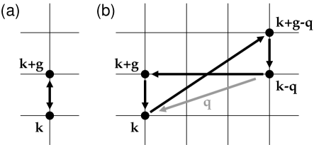
Figure 1: Pattern of couplings between k-points arising in (a) the first term, and (b) the second term, of Eq. (50). Reciprocal vector $\bf q$ is the phonon wavevector, while $\bf g$ is a primitive vector of the k-point mesh (indicated by thin horizontal and vertical lines).

The implementation of the conjugate-gradient minimization algorithm proceeds in a manner very similar to that outlined in Sec. III.1.2. Naively, one would have to work simultaneously with the two search-direction vectors

$$|\zeta_{m{\bf k},{\bf q}}\rangle = \partial F^{(2)}/\partial\langle u^{(1)}_{m{\bf k},{\bf q}}|\;,$$

$$|\zeta_{m{\bf k},-{\bf q}}\rangle = \partial F^{(2)}/\partial\langle u^{(1)}_{m{\bf k},-{\bf q}}|\;,$$ (55)

where $u^{(1)}_{m{\bf k},\pm{\bf q}}$ are the periodic parts of $\psi_{m{\bf k},\pm{\bf q}}^{(1)}$. However, minimizing the second-order energy $F^{(2)}$ with respect to two sets of first-order wavefunctions $u_{n{\bf k},\pm{\bf q}}$ would double the computational cost and would involve substantial restructuring of existing computer codes. We can avoid this by using the fact that the second-order energy is invariant under time reversal to eliminate one set of first-order wavefunctions $\psi_{n{\bf k},-{\bf q}}^{(1)}$ in favor of the other set $\psi_{n{\bf k},{\bf q}}^{(1)}$ following the approach given in Ref. dfpt1, . Specifically, the two sets of first-order wavefunctions are related by

$$\psi_{n{\bf k}}^{(0)}(\bf r) = e^{i\theta_{n{\bf k}}}\psi_{n-{\bf k}}^{(0)*}(\bf r)\;,$$ (56)

$$\psi_{n{\bf k},{\bf q}}^{(1)}\bf r) = e^{i\theta_{n{\bf k}}}\psi_{n-{\bf k},-{\bf q}}^{(1)*}(\bf r)\;,$$ (57)

where $\theta_{n{\bf k}}$ is an arbitrary phase independent of ${\bf r}$. The arbitrary phase $\theta_{n{\bf k}}$ cancels out in the expression of $F^{(2)}$ since every term in $F^{(2)}$ is independent of the phase of the first-order wavefunctions. Thus, we choose $\theta_{n{\bf k}}=1$ for simplicity and write the second-order energy functional in terms of wavefunctions $\psi_{n{\bf k},{\bf q}}$ only.

The minimization procedure now proceeds in a manner similar to the zero-wavevector case, except that the calculation of the Berry-phase part involves some vector-matrix-matrix products as in Eq. (33), but circulating around three of the sides of the loop in Fig. 1. Since $F^{(2)}$ remains in a quadratic form, the minimum of $F^{(2)}$ is again easily searched along the conjugate-gradient direction. Wavefunctions are updated over k-points one after another, and the first-order wavefunctions are updated. This procedure continues until the self-consistent potential is converged. Once the first-order responses of wavefunctions are obtained, the diagonal elements of the dynamical matrix are obtained by evaluating $F^{(2)}$, and the off-diagonal elements are obtained from a straightforward generalization of Eq. (38),

$$\Phi_{\nu\alpha,\mu\beta} = \frac{2\Omega}{(2\pi)^{3}}\int_{\rm BZ}\sum_{m}^{\rm occ}\bigg{(}\langle u_{m{\bf k}}^{(0)}|v_{{\rm ext},\nu\alpha,{\bf k},{\bf k}+{\bf q}}^{(1)}|u^{(1)}_{m{\bf k},\mu\beta,{\bf q}}\rangle$$ (58)

$$+\langle u_{m{\bf k}}^{(0)}|v_{{\rm Hxc},\nu\alpha,{\bf k},{\bf k}+{\bf q}}^{(1)}|u^{(1)}_{m{\bf k},\mu\beta,{\bf q}}\rangle$$

$$+\langle u_{m{\bf k}}^{(0)}|v_{{\rm ext},\nu\alpha,\mu\beta}^{(2)}|u_{m{\bf k}}^{(0)}\rangle\bigg{)}d{\bf k}$$

$$+\frac{1}{2}{E^{(2)}_{\rm Hxc,\nu\alpha,\mu\beta}}\;.$$

IV Test calculations for III-V semiconductors

In order to test our method, we have carried out calculations of the frequency shifts induced by electric fields in two III-V semiconductors, AlAs and GaAs. We have chosen these two materials because they are well-studied systems both experimentally and theoretically, and because the symmetry allows some phonon mode frequencies to shift linearly with electric field while others shift quadratically. Since our main purpose is to check the internal consistency of our theoretical approach, we focus on making comparisons between the shifts calculated using our new linear-response method and those calculated using standard finite-difference methods. Moreover, as mentioned at the start of Sec. II.2.1, we have chosen to neglect changes in phonon frequencies that enter through the electric-field induced strains (piezoelectric and electrostrictive effects), and we do this consistently in both the linear-response and finite-difference calculations. For this reason, our results are not immediately suitable for comparison with experimental measurements.

Our calculations are carried out using a plane-wave pseudopotential approach to density-functional theory. We use the ABINIT code package,abinit which incorporates the finite electric field method of Souza et al.souza02 for the ground-state and frozen-phonon calculations in finite electric field. We then carried out the linear-response calculations with a version of the code that we have modified to implement the linear-response formulas of the previous section.

The details of the calculations are as follows. We use Troullier-Martins norm-conserving pseudopotentials,troullier91 the Teter Pade parameterizationteter96 of the local-density approximation, and a plane-wave cutoff of 16 Hartree. A 10$\times$10$\times$10 Monkhorst-Packmonkhorst76 k-point sampling was used, and we chose lattice constants of 10.62 Å and 10.30 Å for AlAs and GaAs, respectively. The crystals are oriented so that the vector $(a/2)(1,1,1)$ points from a Ga or Al atom to an As atom.

Table 1: Calculated frequency shifts, in cm^-1, induced by an electric field of $5.14\times 10^{8}$ V/m applied along $x$ in GaAs and AlAs. ‘FD’ are the results of finite-difference (frozen-phonon) calculations in which atoms are displaced by hand and restoring forces are calculated, while ‘LR’ refers to the use of the linear-response developed here. The L and X points are at $(2\pi/a)(1,1,1)$ and $(2\pi/a)(1,0,0)$ respectively.

	GaAs		AlAs
Mode	FD	LR	FD	LR
$\Gamma$ O1	$-$3.856	$-$3.856	$-$5.941	$-$5.941
$\Gamma$ O2	$-$0.282	$-$0.281	$-$0.300	$-$0.299
$\Gamma$ O3	3.548	3.548	5.647	5.647
L LO	2.701	2.703	4.282	4.282
L TO1	$-$3.749	$-$3.749	$-$5.663	$-$5.663
L TO2	0.567	0.564	0.952	0.952
X LO	0.050	0.050	$-$0.243	$-$0.243
X TO1	$-$3.953	$-$3.953	$-$6.083	$-$6.083
X TO2	3.753	3.753	5.919	5.919

Table 1 shows the changes in phonon frequencies resulting from an electric field applied along a Cartesian direction at several high-symmetry q-points in GaAs and AlAs. Both the electronic and ionic contributions, Eqs. (7-8), are included. We first relaxed the atomic coordinates in the finite electric field until the maximum force on any atom was less than $10^{-6}$ Hartree/Bohr. We then carried out the linear-response calculation, and in addition, to check the internal consistency of our linear-response method, we carried out a corresponding calculation using a finite-difference frozen-phonon approach. For the latter, the atoms were displaced according to the normal modes obtained from our linear-response calculation, with the largest displacement being 0.0025 Bohr. (Because the electric field lowers the symmetry, the symmetry-reduced set of k-points is not the same as in the absence of the electric field.) The agreement between the finite-different approach and the new linear-response implementation can be seen to be excellent, with the small differences visible for some modes being attributable to truncation in the finite-difference formula and the finite density of the k-point mesh.

In Table 2, we decompose the frequency shifts into the ionic contribution $\Delta\omega_{\rm ion}({\bf q};{\cal E})$ and the electronic contribution $\Delta\omega_{\rm el}({\bf q};{\cal E})$ defined by Eqs. (8) and (7), respectively, calculated using the linear-response approach. It is clear that the largest contributions are ionic in origin. For example, the large, roughly equal and opposite shifts of the O1 and O3 modes at $\Gamma$ arise from the ionic terms. However, there are special cases (e.g., O2 at $\Gamma$ and LO at X) for which the ionic contribution happens to be small, so that the electronic contribution is comparable in magnitude.

The pattern of ionic splittings appearing at $\Gamma$ can be understood as follows. Because the non-analytic long-range Coulomb contribution is not included, the three optical modes at $\Gamma$ are initially degenerate with frequency $\omega_{0}$ in the unperturbed lattice. A first-order electric field along $x$ induces a first-order relative displacement $u_{x}$ of the two sublattices, also along $x$. By symmetry considerations, the perturbed dynamical matrix is given, up to quadratic order in $u_{x}$, as

$$D(\Gamma)=\omega_{0}^{2}\left(\begin{array}[]{ccc}1+\mu u_{x}^{2}&0&0\\ 0&1+\nu u_{x}^{2}&\kappa u_{x}\\ 0&\kappa u_{x}&1+\nu u_{x}^{2}\\ \end{array}\right)\;.$$ (59)

The off-diagonal $\kappa$ term arises from the $E_{xyz}$ coupling in the expansion of the total energy in displacements; this is the only third-order term allowed by symmetry. The $\mu$ and $\nu$ terms arise from fourth-order couplings of the form $E_{xxxx}$ and $E_{xxyy}$ respectively. The eigenvalues of this matrix are proportional to $1+\mu u_{x}^{2}$ and $1\pm\kappa u_{x}+\nu u_{x}^{2}$. Thus, two of the modes should be perturbed at first order in the field-induced displacements with a pattern of equal and opposite frequency shifts, while all three modes should have smaller shifts arising from the quadratic terms. This is just what is observed in the pattern of frequency shifts shown in Table 2. (The symmetry of the pattern of electronic splittings is the same, but it turns out that the linear shift is much smaller in this case, so that for the chosen electric field, the linear and quadratic contributions to the electronic frequency shift have similar magnitudes.) A similar analysis can be used to understand the patterns of frequency shifts at the $L$ and $X$ points.

Table 2: Same as in Table 1, but with the frequency shifts decomposed into ionic and electronic contributions as defined in Eqs. (8) and (7) respectively.

	GaAs		AlAs
	Ion	Elec.	Ion	Elec.
$\Gamma$ O1	$-$3.659	$-$0.198	$-$5.684	$-$0.257
$\Gamma$ O2	$-$0.146	$-$0.135	$-$0.123	$-$0.177
$\Gamma$ O3	3.655	$-$0.107	5.589	0.058
L LO	2.341	0.362	3.633	0.649
L TO1	$-$3.486	$-$0.262	$-$5.628	$-$0.034
L TO2	1.181	$-$0.617	1.658	$-$0.707
X LO	0.122	$-$0.073	$-$0.033	$-$0.209
X TO1	$-$3.411	$-$0.543	$-$5.658	$-$0.424
X TO2	3.388	0.365	5.609	0.310

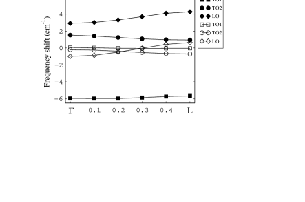
Figure 2: Frequency shifts induced by an electric field of 5.14$\times 10^{8}$ V/m along $x$ in AlAs, plotted along $\Gamma$ to $L$. Filled and open symbols indicate the total shift $\Delta\omega_{\rm el}+\Delta\omega_{\rm ion}$ and the electronic contribution $\Delta\omega_{\rm el}$ respectively.

We have also plotted, in Fig. 2, the calculated total frequency shift $\Delta\omega_{\rm el}({\bf q})+\Delta\omega_{\rm ion}({\bf q})$ and its electronic contribution $\Delta\omega_{\rm el}({\bf q})$ along the line from $\Gamma$ to L for the case of AlAs. (The ‘LO’ and ‘TO’ symmetry labels are not strictly appropriate here because the electric field along $x$ mixes the mode eigenvectors; the notation indicates the mode that would be arrived at by turning off the field.) In contrast to the results presented in Tables 1-2, the frequencies at $\Gamma$ in Fig. 2 were computed by including the long-range non-analytic Coulomb contribution for $\hat{q}\parallel(111)$ in order to extend the curves to $q=0$. (Because the direct linear-response calculation of the dynamical effective charge and dielectric susceptibility tensors are not yet developed and implemented in the presence of a finite electric field, the needed tensor elements were computed by finite differences.) It is clearly evident that the electronic terms remain much smaller than the ionic ones for all three optical modes over the entire branch in $q$-space.

Table 3: Comparison of ionic displacements and frequency shifts at the $L$ point in GaAs as computed by the approximate and exact approaches of Sec. II.2.2 and II.2.1 respectively, again for an electric field of $5.14\times 10^{8}$ V/m along $x$. $R_{{\cal E}}$ is the induced displacement of the cation sublattice along $x$, and the $\Delta\omega_{\rm ion}$ are ionic contributions to the frequency shifts as defined in Eq. (8).

		$R_{{\cal E}}$	$\Delta\omega_{\rm ion}$(L) (cm-1)
		(10-3 Å)	LO	TO1	TO2
GaAs	Approx.	5.07	2.63	$-$3.89	1.37
	Exact	4.95	2.34	$-$3.49	1.18
AlAs	Approx.	5.69	3.75	$-$5.66	1.65
	Exact	5.62	3.63	$-$5.63	1.66

Returning now to the comparison between our exact theory of Sec. II.2.1 and the approximate theory of Sec. II.2.2, we compare the equilibrium positions and phonon frequencies predicted by these theories in Table 3. Recall that $R_{{\cal E}}$ is calculated in the approximate theory by using Eq. (10). Using this force, the ion coordinates were again relaxed to a tolerance of $10^{-6}$ (Hartree/Bohr) on the forces. It can be seen that $R_{{\cal E}}$ is predicted quite well by the approximate theory, with errors of only $\sim$2%, confirming that the displacements can be calculated to good accuracy using a linearized theory for this magnitude of electric field. The changes in the phonon frequencies resulting from these displacements (evaluated at zero and non-zero field for the approximate and exact theories respectively) are listed in the remaining columns of Table 3. The discrepancies in the phonon frequencies are now somewhat larger, approaching 15% in some cases. This indicates that the approximate theory is able to give a moderately good description of the phonon frequency shifts of GaAs in this field range, but the exact theory is needed for accurate predictions. (Also, recall that the approximate theory does not provide any estimate for the electronic contributions, which are not included in Table 3.)

Finally, we illustrate our ability to calculate the nonlinear field dependence of the phonon frequencies by presenting the calculated optical $L$-point phonon frequencies of AlAs in Fig. 3 as a function of electric field along $x$. These are again the results of our exact theory, obtained by including both ionic and electronic contributions. The two TO modes are degenerate at zero field, as they should be. All three modes show a linear component that dominates their behavior in this range of fields. However, a quadratic component is also clearly evident, illustrating the ability of the present approach to describe such nonlinear behavior.

Figure 3: Frequencies of LO and TO modes at $L$ in AlAs as a function of electric field (where 10^-3 a.u. = $5.14\times 10^{8}$ V/m) applied along $x$. The symbols have the same interpretation as in Fig. 2.

V Summary and discussion

We have developed a method for computing the phonon frequencies of an insulator in the presence of a homogeneous, static electric field. The extension of density-functional perturbation theory to this case has been accomplished by carrying out a careful expansion of the field-dependent energy functional $E_{\rm KS}+\Omega{\cal E}\cdot{\bf P}$, where ${\bf P}$ is the Berry-phase polarization, with respect to phonon modes both at $q=0$ and at arbitrary $q$. In the general case of nonzero $q$, there is a subtle interplay between the couplings between neighboring k-points introduced by the electric field and the further-neighbor couplings introduced by the $q$-vector, so that terms arise that require the evaluation of four-sided loops in k-space. However, with the judicious use of time-reversal symmetry, the needed evaluations can be reduced to a form that is not difficult to implement in an existing DFPT code.

We have carried out test calculations on two III-V semiconductors, AlAs and GaAs, in order to test the correctness of our implementation. A comparison of the results of linear-response and finite-difference calculations shows excellent agreement, thus validating our approach. We also decompose the frequency shifts into “lattice” and “electronic” contributions and quantify these, and we find that the lattice contributions (i.e., those resulting from induced displacements in the reference equilibrium structure) are usually, but not always, dominant. We also evaluated the accuracy of an approximate method for computing the lattice contribution, in which only zero-field inputs are needed. We found that this approximate approach gives a good rough description, but that the full method is needed for an accurate calculation.

Our linear-response method has the same advantages, relative to the finite-difference approach, as in zero electric field. Even for a phonon at $\Gamma$, our approach is more direct and simplifies the calculation of the phonon frequencies. However, its real advantage is realized for phonons at arbitrary $q$, because the frequency can still be obtained efficiently from a calculation on a single unit cell without the need for imposing commensurability of the $q$-vector and computing the mode frequencies for the corresponding supercell. We also emphasize that the method is not limited to infinitesimal electric fields. We thus expect the method will prove broadly useful for the study of linear and nonlinear effects of electric bias on the lattice vibrational properties of insulating materials.

Appendix

The formula for the electric polarization given in the original work of King-Smith and Vanderbiltsmith93 is not a suitable starting point for the phonon perturbation analysis that we wish to derive here, because a perturbation of nonzero wavevector ${\bf q}$ acting on a Bloch function generates a wavefunction that is no longer of Bloch form. That is, while the zero-order wavefunction $\psi^{(0)}_{m{\bf k}}$ transforms as $e^{i{\bf k}\cdot{\bf R}}$ under a translation by ${\bf R}$, the first-order wavefunction $\psi^{(1)}_{m{\bf k},{\bf q}}$ transforms as $e^{i({\bf k}+{\bf q})\cdot{\bf R}}$.

To solve this problem, we first restrict ourselves to the case of a regular mesh of $N=N_{1}\times N_{2}\times N_{3}$ k-points in the Brillouin zone. As is well known, one can regard the Bloch functions at these k-points as being the solutions at a single k-point of the downfolded Brillouin zone of an $N_{1}\times N_{2}\times N_{3}$ supercell. Then, as long as the wavevector ${\bf q}$ is a reciprocal lattice vector of the supercell, or ${\bf q}=m_{1}{\bf b}_{1}/N_{1}+m_{2}{\bf b}_{2}/N_{2}+m_{3}{\bf b}_{3}/N_{3}$, the phonon perturbation will be commensurate with the supercell, and the perturbed wavefunction will continue to be a zone-center Bloch function of the supercell. We thus restrict our analysis to this case.

A formula for the Berry-phase polarization for single-k-point sampling of a supercell has been provided by Resta.resta98 Starting from a general many-body formulation in terms of a definition of the position operator suitable for periodic boundary conditions, and then specializing to the case of a single-particle Hamiltonian, Resta’s derivation leads to

$${\bf P}=\frac{ef}{2\pi\Omega}\sum_{\alpha}\gamma_{\alpha}\,{\bf a}_{\alpha}$$ (60)

where the Berry phase in lattice direction $\alpha$ is given by

$$\gamma_{\alpha}=-\textrm{Im}\,\ln\det M_{\alpha}\;.$$ (61)

Here

$$M_{\alpha,ss^{\prime}}=\langle\psi_{s}|e^{-i{\bf g}_{\alpha}\cdot{\bf r}}|\psi_{s^{\prime}}\rangle$$ (62)

where ${\bf g}_{\alpha}={\bf b}_{\alpha}/N_{\alpha}$ is the primitive reciprocal mesh vector in lattice direction $\alpha$ and $s$ runs over all of the occupied states of the supercell. Expanding the matrix $M_{\alpha}$ in powers of $\lambda$ and $\lambda^{*}$,

$$M_{\alpha}(\lambda,\lambda^{*}) = M_{\alpha}^{(0,0)}+\lambda M_{\alpha}^{(1,0)}+\lambda^{*}M_{\alpha}^{(0,1)}+\lambda^{2}M_{\alpha}^{(2,0)}$$ (63)

$$+|\lambda|^{2}M_{\alpha}^{(1,1)}+\lambda^{*2}M_{\alpha}^{(0,2)}+...\;,$$

the expansion of $\ln\det M_{\alpha}(\lambda,\lambda^{*})$ takes the form nunes01

$$\ln\det M_{\alpha} = \ln\det M_{\alpha}^{(0,0)}$$ (64)

$$+ \lambda\,\textrm{Tr}[M_{\alpha}^{(1,0)}Q_{\alpha}]+\lambda^{*}\,\textrm{Tr}[M_{\alpha}^{(0,1)}Q_{\alpha}]$$

$$+ \lambda^{2}\,\textrm{Tr}[2M_{\alpha}^{(2,0)}Q_{\alpha}-M_{\alpha}^{(1,0)}Q_{\alpha}M_{\alpha}^{(1,0)}Q_{\alpha}]$$

$$+ \lambda^{*2}\,\textrm{Tr}[2M_{\alpha}^{(0,2)}Q_{\alpha}-M_{\alpha}^{(0,1)}Q_{\alpha}M_{\alpha}^{(0,1)}Q_{\alpha}]$$

$$+ |\lambda|^{2}\,\textrm{Tr}[2M_{\alpha}^{(1,1)}Q_{\alpha}-M_{\alpha}^{(1,0)}Q_{\alpha}M_{\alpha}^{(0,1)}Q_{\alpha}$$

$$\qquad\qquad-M_{\alpha}^{(0,1)}Q_{\alpha}M_{\alpha}^{(1,0)}Q_{\alpha}]$$

$$+ \textrm{higer order terms}\;,$$

where $Q_{\alpha}=[M_{\alpha}^{(0,0)}]^{-1}$.

From the physical point of view, the terms proportional to $\lambda$, $\lambda^{*}$, $\lambda^{2}$, and $\lambda^{*2}$ should vanish as a result of translational symmetry. For example, a term linear in $\lambda$ should transform like $e^{i{\bf q}\cdot{\bf R}}$ under translation by a lattice vector ${\bf R}$, but such a form is inappropriate in an expression for the energy, which must be an invariant under translation. We have confirmed this by explicitly carrying out the matrix multiplications for these terms and checking that the traces are zero. Using the cyclic property of the trace to combine the last two terms, we find that the overall second-order change in $\ln\det M_{\alpha}$ is

$$(\ln\det M_{\alpha})^{(2)} = 2|\lambda|^{2}\,\textrm{Tr}[M_{\alpha}^{(1,1)}Q_{\alpha}$$ (65)

$$\quad-M_{\alpha}^{(1,0)}Q_{\alpha}M_{\alpha}^{(0,1)}Q_{\alpha}]\;.$$

In our case, the orbitals $\psi_{s}$ appearing in Eq. (62) are the perturbed wavefunctions originating from the unperturbed states labeled by band $m$ and k-point ${\bf k}$ of the primitive cell, so that we can let $\psi_{s}\rightarrow\psi_{m{\bf k}}$ and

$$M_{\alpha,m{\bf k},m^{\prime}{\bf k}^{\prime}}=\langle\psi_{m{\bf k}}|e^{-i{\bf g}_{\alpha}\cdot{\bf r}}|\psi_{m^{\prime}{\bf k}^{\prime}}\rangle\;.$$ (66)

Substituting Eq. (43) into Eq. (66), we find

$$M_{\alpha,m{\bf k},m^{\prime}{\bf k}^{\prime}}^{(1,0)} = \langle\psi_{m{\bf k}}^{(0)}|e^{-i{\bf g}_{\alpha}\cdot{\bf r}}|\psi_{m^{\prime}{\bf k}^{\prime},{\bf q}}^{(1)}\rangle$$ (67)

$$+\langle\psi_{m{\bf k},-{\bf q}}^{(1)}|e^{-i{\bf g}_{\alpha}\cdot{\bf r}}|\psi_{m^{\prime}{\bf k}^{\prime}}^{(0)}\rangle\;,$$

$$M_{\alpha,m{\bf k},m^{\prime}{\bf k}^{\prime}}^{(0,1)} = \langle\psi_{m{\bf k}}^{(0)}|e^{-i{\bf g}_{\alpha}\cdot{\bf r}}|\psi_{m^{\prime}{\bf k}^{\prime},-{\bf q}}^{(1)}\rangle$$ (68)

$$+\langle\psi_{m{\bf k},{\bf q}}^{(1)}|e^{-i{\bf g}_{\alpha}\cdot{\bf r}}|\psi_{m^{\prime}{\bf k}^{\prime}}^{(0)}\rangle\;,$$

$$M_{\alpha,m{\bf k},m^{\prime}{\bf k}^{\prime}}^{(1,1)} = \langle\psi_{m{\bf k},{\bf q}}^{(1)}|e^{-i{\bf g}_{\alpha}\cdot{\bf r}}|\psi_{m^{\prime}{\bf k}^{\prime},{\bf q}}^{(1)}\rangle$$ (69)

$$+\langle\psi_{m{\bf k},-{\bf q}}^{(1)}|e^{-i{\bf g}_{\alpha}\cdot{\bf r}}|\psi_{m^{\prime}{\bf k}^{\prime},-{\bf q}}^{(1)}\rangle\;,$$

and $Q_{\alpha}=[M_{\alpha}^{(0,0)}]^{-1}$ where

$$M_{\alpha,m{\bf k},m^{\prime}{\bf k}^{\prime}}^{(0,0)}=\langle\psi_{m{\bf k}}^{(0)}|e^{-i{\bf g}_{\alpha}\cdot{\bf r}}|\psi_{m^{\prime}{\bf k}^{\prime}}^{(0)}\rangle\;.$$ (70)

The transformation properties of the zero- and first-order wavefunctions under translations, given by Eqs. (46) and (45), impose sharp constraints upon which of the terms in Eqs. (67-70) can be non-zero. For example, for $M_{\alpha}^{(1,0)}$ in Eq. (67), the term $\langle\psi_{m{\bf k}}^{(0)}|e^{-i{\bf g}_{\alpha}\cdot{\bf r}}|\psi_{m^{\prime}{\bf k}^{\prime},{\bf q}}^{(1)}\rangle$ is only non-zero if ${\bf k}={\bf k}^{\prime}+{\bf q}-{\bf g}_{\alpha}$. Similarly, $Q_{\alpha,m{\bf k},m^{\prime}{\bf k}^{\prime}}$ is only non-zero if ${\bf k}={\bf k}^{\prime}+{\bf g}_{\alpha}$. In practice, we define primitive-cell-periodic functions

$$u_{m{\bf k}}^{(0)}({\bf r})=e^{-i{\bf k}\cdot{\bf r}}\psi_{m{\bf k}}^{(0)}({\bf r})$$ (71)

and

$$u_{m{\bf k},{\bf q}}^{(1)}({\bf r})=e^{-i({\bf k}+{\bf q})\cdot{\bf r}}\psi_{m{\bf k},{\bf q}}^{(1)}({\bf r})$$ (72)

so that

$$M_{\alpha,m{\bf k},m^{\prime}{\bf k}^{\prime}}^{(1,0)} = S_{{\bf k}{\bf k}^{\prime},mm^{\prime}}^{(1,0)}\,\delta_{{\bf k},{\bf k}^{\prime}+{\bf q}-{\bf g}_{\alpha}}\;,$$

$$M_{\alpha,m{\bf k},m^{\prime}{\bf k}^{\prime}}^{(0,1)} = S_{{\bf k}{\bf k}^{\prime},mm^{\prime}}^{(0,1)}\,\delta_{{\bf k},{\bf k}^{\prime}-{\bf q}-{\bf g}_{\alpha}}\;,$$

$$M_{\alpha,m{\bf k},m^{\prime}{\bf k}^{\prime}}^{(1,1)} = S_{{\bf k}{\bf k}^{\prime},mm^{\prime}}^{(1,1)}\,\delta_{{\bf k},{\bf k}^{\prime}-{\bf g}_{\alpha}}\;,$$

$$M_{\alpha,m{\bf k},m^{\prime}{\bf k}^{\prime}}^{(0,0)} = S_{{\bf k}{\bf k}^{\prime},mm^{\prime}}^{(0,0)}\,\delta_{{\bf k},{\bf k}^{\prime}-{\bf g}_{\alpha}}\;,$$ (73)

where

$$S_{{\bf k}{\bf k}^{\prime},mm^{\prime}}^{(1,0)} = \langle u_{m{\bf k}}^{(0)}|u_{m^{\prime}{\bf k}^{\prime},{\bf q}}^{(1)}\rangle+\langle u_{m{\bf k},-{\bf q}}^{(1)}|u_{m^{\prime}{\bf k}^{\prime}}^{(0)}\rangle\;,$$

$$S_{{\bf k}{\bf k}^{\prime},mm^{\prime}}^{(0,1)} = \langle u_{m{\bf k}}^{(0)}|u_{m^{\prime}{\bf k}^{\prime},-{\bf q}}^{(1)}\rangle+\langle u_{m{\bf k},{\bf q}}^{(1)}|u_{m^{\prime}{\bf k}^{\prime}}^{(0)}\rangle\;,$$

$$S_{{\bf k}{\bf k}^{\prime},mm^{\prime}}^{(1,1)} = \langle u_{m{\bf k},{\bf q}}^{(1)}|u_{m^{\prime}{\bf k}^{\prime},{\bf q}}^{(1)}\rangle+\langle u_{m{\bf k},-{\bf q}}^{(1)}|u_{m^{\prime}{\bf k}^{\prime},-{\bf q}}^{(1)}\rangle\;,$$

$$S_{{\bf k}{\bf k}^{\prime},mm^{\prime}}^{(0,0)} = \langle u_{m{\bf k}}^{(0)}|u_{m^{\prime}{\bf k}^{\prime},{\bf q}}^{(0)}\rangle$$ (74)

(subscript $\alpha$ is now implicit). Defining $Q_{{\bf k}^{\prime}{\bf k}}=[S_{{\bf k}{\bf k}^{\prime}}^{(0,0)}]^{-1}$ and taking into account the constraints on k-points embodied in the delta functions in Eq. (73), the two terms in Eq. (65) become

$$\textrm{Tr}[M_{\alpha}^{(1,1)}Q_{\alpha}]=\sum_{\bf k}\textrm{Tr}[S^{(1,1)}_{{\bf k},{\bf k}+{\bf g}}Q_{{\bf k}+{\bf g},{\bf k}}]$$ (75)

and

$$\textrm{Tr}[M_{\alpha}^{(1,0)}Q_{\alpha}M_{\alpha}^{(0,1)}Q_{\alpha}]=\sum_{\bf k}\textrm{Tr}[S^{(1,0)}_{{\bf k},{\bf k}+{\bf g}-{\bf q}}$$

$$\qquad\times Q_{{\bf k}+{\bf g}-{\bf q},{\bf k}-{\bf q}}S^{(0,1)}_{{\bf k}-{\bf q},{\bf k}+{\bf g}}Q_{{\bf k}+{\bf g},{\bf k}}]\;.$$ (76)

In these equations, the trace on the left-hand side is over all occupied states of the supercell, while on the right-hand side it is over bands of the primitive cell. These are the terms that appear in Eq. (50) in the main text, and that determine the pattern of k-point loops illustrated in Fig. 1.

References

- (1) K. Parlinski, Z-.Q. Li, and Y. Kawazoe, Phys. Rev. Lett. 78, 4063(1997).
- (2) K. Kunc and Richard M. Martin, Phys. Rev. Lett. 48, 406 (1982).
- (3) P. Giannozzi, S. de Gironcoli, P. Pavone, and S. Baroni, Phys. Rev. B 43, 7231 (1991).
- (4) X. Gonze and C. Lee, Phys. Rev. B 55, 10355 (1997).
- (5) X. Gonze, Phys. Rev. B 55, 10337 (1997).
- (6) S. Baroni, S. de Gironcoli, A. Dal Corso and P. Giannozzi, Rev. Mod. Phys. 73, 515 (2001).
- (7) I. Souza, J. Íñiguez, and D. Vanderbilt, Phys. Rev. Lett. 89, 117602 (2002).
- (8) P. Umari and A. Pasquarello, Phys. Rev. Lett. 89, 157602 (2002).
- (9) R.D. King-Smith and D. Vanderbilt, Phys. Rev. B 47, 1651 (1993).
- (10) N. Sai, K.M. Rabe, D. Vanderbilt, Phys. Rev. B 66, 104108 (2002).
- (11) Huaxiang Fu and L. Bellaiche, Phys. Rev. Lett. 91, 57601 (2003).
- (12) Ivan I. Naumov and Huaxiang Fu, Phys. Rev. B 72, 012304 (2005).
- (13) A. Antons, J.B. Neaton, K.M. Rabe, and D. Vanderbilt, Phys. Rev. B 71, 024102 (2005).
- (14) O. Diéguez and D. Vanderbilt, Phys. Rev. Lett. 96, 056401 (2006).
- (15) X. Gonze, Phys. Rev. B 52, 1096 (1995).
- (16) R.W. Nunes and X. Gonze, Phys. Rev. B 63, 155107 (2001).
- (17) M.C. Payne, M.P. Teter, D.C. Allan, T.A. Arias and J.D. Joannopoulos, Rev. Mod. Phys. 64, 1045 (1992).
- (18) R. Resta, Phys. Rev. Lett. 80, 1800 (1998).
- (19) The ABINIT code is a common project of the Université Catholique de Louvain, Corning Incorporated, and other contributors (www.abinit.org). See: X. Gonze and others, Comp. Mat. Science 25, 478 (2002).
- (20) N. Troullier and J.L. Martins, Phys. Rev. B 43, 1993 (1991).
- (21) S. Goedecker, M. Teter and J. Hutter, Phys. Rev. B 54, 1703 (1996).
- (22) H.J. Monkhorst and J.D. Pack, Phys. Rev. B 13, 5188 (1976).