Interacting Bose gases in quasi-one dimensional optical lattices

Abstract

We study a two-dimensional array of coupled one-dimensional (1D) tubes of interacting bosons. Such systems can be produced by loading ultra-cold atoms in anisotropic optical lattices. We investigate the effects of coupling the tubes via hopping of the bosons (i.e. Josephson coupling). In the absence of a periodic potential along the tubes, or when such potential is incommensurate with the boson density, the system undergoes a transition from an array of incoherentTomonaga-Luttinger liquids at high temperature to an anisotropic Bose-Einstein condensate (BEC), at low temperature. We determine the transition temperature and long wave-length excitations of the BEC. In addition to the usual gapless (Goldstone) mode found in standard superfluids, we also find a gapped mode associated with fluctuations of the amplitude of the order parameter. When a commensurate periodic potential is applied along the tubes, they can become 1D Mott insulators. Intertube hopping leads to a deconfinement quantum phase transition between the 1D Mott insulators and the anisotropic BEC. We also take into account the finite size of the gas tubes as realized in actual experiments. We map out the phase diagram of the quasi-1D lattice and compare our results with the existing experiments on such systems.

1 Introduction

One dimension (1D) provides fertile grounds for studying the physics of strongly correlated quantum many-body systems. It is a well established theoretical result that, because of the enhanced role of quantum fluctuations in low dimensionality, there is no broken continuous symmetry and therefore long range order, even at zero temperature, in a 1D quantum many body system. Instead, in a large class of systems possessing a gapless spectrum, power laws characterize the various correlation functions. This class of systems is known as a Tomonaga-Luttinger liquid (TLL).

One of the simplest examples of a TLL is the Lieb-Liniger model [1], which describes a system of non-relativistic bosons interacting via a contact (Dirac delta-function) potential. This model has been solved exaclty using the Bethe ansatz [1], which has provided valuable insights into its thermodynamic properties and excitation spectrum. However, calculation of the asymptotics of correlation functions is not an easy task using this method, and in this regard it is nicely complemented by the harmonic-fluid approach introduced by Haldane [2]. The combination of these two methods has allowed us to understand that, as the the interaction is increased, the system exhibits no quantum phase transition. Instead, it smoothly crosses over from a weakly interacting (often called quasi-condensate [3, 4, 5]) regime, where phase fluctuations decay very slowly, to a strongly interacting regime, the Tonks regime [6]. In the latter, repulsion between the bosons is so strong that it leads to an effective exclusion principle in position space, and makes the system resemble a gas of non-interacting spinless fermions in many properties. Thus it is sometimes stated that the bosons in the Tonks regime “fermionize”.

This very simple model solved by Lieb and Liniger in 1963 has recently received a great deal of attention thanks to spectacular advances in confining quantum degenerate gases of alkali atoms in low dimensional traps [7]. While at the beginning only weakly interacting 1D Bose gases were available [8, 9], the application of a deep optical potential parallel to the 1D axis to arrays of 1D Bose gases has recently allowed the group at ETH (Zürich) [10, 11] to demonstrate a quantum phase transition from a superfluid TLL to a 1D Mott insulator, which is the low dimensional analog of the superfluid to Mott insulator transition first demonstrated in the 3D optical lattice by Greiner and coworkers [12]. Furthermore, Kinoshita et al. [13] have succeeded in reaching the Tonks regime by creating an array of tightly confined 1D Bose gases. A different path [14, 15] to realize a strongly interacting 1D Bose gases has been followed by Paredes et al. [16], who applied a deep periodic potential to an array of (otherwise weakly interacting) 1D Bose gases. Thus they were able to dramatically increase the ratio of the interaction to the kinetic energy of the atoms. In both cases [13, 16], the observation of fermionization signatures was reported.

In the past, much experimental effort focusing on low dimensional systems has been spent on studying electronic systems such as spin chains and quasi-1D metals (for a review see [17]). Theoretically at least, electrons in 1D become a TLL (provided there are no gap-opening perturbations) as soon as interactions are taken into account in a non-perturbative way. However, for the electronic systems comparison between theory and experiment has proved problematic partly because of material-specific issues such as the existence of many competing phenomena at similar energy scales (e.g. in Bechgaard salts [18, 19]) or the always-present disorder in solid state systems [17]. Furthermore, one major complication stems from the fact that these materials are indeed three dimensional (3D), as there is always a small amplitude for electrons to hop from chain to chain, whereas Coulomb interactions (often poorly screened because of bad metallicity) also enhance 3D ordering tendencies. These inter-chain couplings cannot be neglected at low temperatures, which leads to the interesting physics of dimensional crossover: at temperatures high compared to the energy scale determined by these inter-chain couplings, the system effectively behaves as a collection of isolated 1D chains. However, when the temperature is lowered below this scale, 3D coherence develops between the chains and, at zero temperature, a complete 3D description of the system is required. Much exciting physics is expected to occur in this crossover from the exotic 1D TLL state to a conventional 3D (but strongly anisotropic) Fermi liquid, or an ordered 3D phase [17]. Indeed, these phenomena may well have relevance to the pseudogap (and other anomalous) behavior of the quasi-2D high temperature superconductor materials. For instance, one of the many interesting questions that arise in this context is the following: how [19] do the exotic low-energy excitations (bosonic collective modes) of the 1D system transform into the Landau quasi-particles characteristic of Fermi liquids and which resemble more the constituent electrons?

The dimensional crossover phenomena described above has also a counterpart in Bose gases loaded in quasi-1D optical lattices. From a theoretical point of view, the fact that bosons can undergo Bose-Einstein condensation and, therefore, can be collectively described using a macroscopic quantum field makes more amenable these systems to a theoretical analysis relying on a mean field approximation. Such a mean-field analysis is undertaken in this work: here we treat the intertube hopping via a mean field approximation, while quantum fluctuations within a tube are treated accurately at low energies using the harmonic-fluid approach.

From the experimental point of view, the recent availability of gases of ultra-cold bosonic atoms in optical lattices has revived the interest in understanding the properties of coupled systems of bosons in 1D. Furthermore, the already demonstrated high degree of tunability of these systems can provide a clean setup to study the physics of dimensional crossover. Thus, as we show in section 3 of this work, the phenomenology of Bose-Einstein condensation in the most anisotropic version of these lattices is very different from the one exhibited by Bose gases condensing in the absence of a lattice or even in shallow isotropic optical lattices.

In addition to studying the properties of Bose condensed systems in lattices, some experimental groups have applied a tunable optical potential along the longitudinal direction of an array of effectively uncoupled 1D Bose gases. It has been thus possible [10], as mentioned above, to drive a quantum phase transition from the 1D superfluid (TLL) state to a 1D Mott insulator. Under these circumstances, the effect of a small hopping amplitude (i.e. Josephson coupling) between neighboring tubes in the array becomes most interesting: as we show in section 4, for a finite value of the hopping amplitude, the system undergoes a new type of quantum phase transition, known as “deconfinement” transition, from the 1D Mott insulator to an anisotropic Bose-Einstein condensate. Thus the tendency of bosons to develop phase coherence overcomes the localization effect of the optical potential. As explained in section 6, we believe that some features of this deconfinement transition may have been observed in the experiments of Ref. [10].

This paper is organized as follows: section 2 defines our model of a 2D array of 1D tubes of bosons coupled by weak intertube tunneling, and describes the harmonic-fluid approach that allows us to derive a low-energy effective Hamiltonian. Then we discuss separately the phenomenon of Bose-Einstein condensation and the properties of the condensate in an anisotropic lattice (section 3), and the deconfinement quantum phase transition (section 4). In the former case, we obtain the zero-temperature condensate fraction, the condensation temperature, and the excitations of the condensate using the mean field approximation and including gaussian fluctuations about the mean field state. We also show that some of the results obtained by these methods are recovered from the self-consistent harmonic approximation (section 3.2). These calculations are described in pedagogical detail in A, B, and C. Moreover, in section 3.1.3 we discuss the excitation spectrum of the Bose-condensed phase, and in particular the existence of a gapped mode related to oscillations of the amplitude of the condensate fraction, in the light of a phenomenological Ginzburg-Landau theory. Differences between this theory and the more conventional Gross-Pitaevskii theory, where the gapped mode is absent, are exhibited. The transition from the (anisotropic) regime described by the Ginzburg-Landau theory to the one where Gross-Pitaeskii theory holds is also outlined there.

The deconfinement transition is described in section 4. There we show how the renormalization group can be used to understand the competition between the localization in the optical potential and a small tunneling amplitude between neighboring 1D Bose systems. To assess the nature of the deconfinement transition, we map (see section 4.2) the mean-field Hamiltonian, at a specific value of the system’s parameters, to a spin-chain model. Finally, section 5 discusses the effect of the finite size of the 1D system that are realized in actual experiments, and how it modifies the phase diagram obtained from the renormalization-group analysis. We argue that, for an array of finite 1D Bose gases, there is a extra energy scale below which the tunneling of atoms between tubes is effectively blocked. Finally, in section 6 we present a discussion of the experimental observations and how they compare with the predictions of our theory. A brief account of some of our results has appeared elsewhere [20].

2 Models and Bosonization

In this section we introduce the models for an interacting Bose gas in a quasi-1D optical lattice that we study in the rest of the paper. We also briefly describe the harmonic-fluid approach (henceforth referred to as “bosonization”), which allows us to obtain a convenient effective low-temperature description of these models.

2.1 Models of a Bose gas in a quasi-1D optical lattice

In this work we study the low-temperature equilibrium properties of systems recently realized by several experimental groups [7, 13, 10, 16, 21, 22, 23] which have succeeded in loading ultracold atomic gases in highly anisotropic (quasi-1D) optical lattices. In the experiments carried out by these groups, a Bose-Einstein condensate of ultracold alkali atoms (in particular, ⁸⁷Rb) is placed in a region of space where two pairs of non-coherent and mutually orthogonal counter-propagating lasers intersect. The intensity of the lasers is increased adiabatically, and because of the AC stark effect, the atoms experience a periodic potential [24] $V_{\perp}(y,z)=V_{0y}\sin^{2}\left(2\pi y/\lambda\right)+V_{0z}\sin^{2}\left(2\pi z/\lambda\right)$, where usually $V_{0y}=V_{0z}=V_{0\perp}$, with $V_{0\perp}\propto E^{2}_{0}$, $E_{0}$ being the maximum intensity of the electric field of a laser whose wavelength is $\lambda$. The strength of the optical potential, $V_{0\perp}$, is frequently given in units of the recoil energy, $E_{R}=\hbar^{2}\pi^{2}/(2Ma^{2})$, where $a=\lambda/2$ is the period of $V_{\perp}(y,z)$ and $M$ the atom mass . For $V_{0\perp}\gg\mu_{3D}$, where $\mu_{3D}\approx 4\pi\hbar^{2}a_{s}\rho^{3D}_{0}/M$ [25] is the chemical potential of the BEC ($a_{s}$ being the s-wave scattering length of the atom-atom interaction potential, and $\rho^{3D}_{0}$ the mean atom density), the gas atoms are mainly confined to the minima of $V_{\perp}(x,y)$, thus forming long, effectively 1D, gas tubes as shown in figure 1 (there are additional harmonic potentials along the $x,y,z$-axes that trap the atoms). Under these conditions, we can project the boson field operator $\Psi(x,y,z)$ onto the lowest (Bloch) band of the periodic potential,

$$\Psi(x,y,z)\simeq\sum_{{\bf R}}W_{\bf R}(y,z)\>\Psi_{\bf R}(x),$$ (1)

where ${\bf R}=(m_{y},m_{z})\>a$, with integers $m_{i}=-M_{i}/2,\ldots,+M_{i}/2$ ($i=y,z$), is the location of the different potential minima; $W_{\bf R}(x,y)$ is the Wannier function of the lowest Bloch band centered around $\bf R$. The system just described is called a 2D (square) optical lattice. In typical experiments $M_{y}\sim M_{z}\sim 10^{2}$, and thus the number of gas tubes is of the order of a few thousand separated half a laser of wave-length, $\lambda/2\simeq 0.4\,\mu{\rm m}$.

In addition, in several of the experiments [10, 22, 16] an extra pair of lasers was applied to define a longitudinal periodic potential $V_{||}(x)=V_{0||}\sin^{2}\left(2\pi x/\lambda\right)=\frac{1}{2}V_{0||}+u(x)$, and $u(x)=u_{0}\>\cos(Gx)$, where $u_{0}=-V_{0||}/2$ and $G=4\pi/\lambda=2\pi/a$. Since, for a commensurate potential, i.e. when the period $a$ matches the mean interparticle distance, the variation of the strength of $u(x)$ is responsible for the transition [2, 26, 17] to a Mott insulating state where the bosons are localized, we shall henceforth refer to $u(x)$ as the “Mott potential”. In this work we are interested in the extreme anisotropic case where the strength of this potential $|u_{0}|\sim V_{0||}\ll V_{0\perp}$. In experiments, this was achieved by increasing $V_{0\perp}$ so that the motion of the atoms effectively becomes confined to a one-dimensional tube, where they undergo only zero-point motion in the transverse directions. This picture is equivalent to the projection onto the lowest Bloch band described above. Just like in three dimensional space, the atomic interactions in the tube are still well described by a Dirac-delta pseudo-potential, $v_{a}(x)=g_{1D}\>\delta(x)$, where the effective coupling $g_{1D}$ has been obtained in Ref. [27]:

$$g_{\rm 1D}=\frac{2\hbar^{2}a_{s}}{(1-{\cal C}a_{s}/\sqrt{2}\ell_{\perp})M\ell^{2}_{\perp}}.$$ (2)

The constant ${\cal C}\simeq 1.4603$, and the oscillator length in the transverse direction, $\ell_{\perp}=\left(\hbar/(M\omega_{\perp})\right)^{1/2}$ (where $\hbar\omega_{\perp}/E_{R}\simeq 2(V_{0\perp}/E_{R})^{1/2}$ for deep lattices [12], is the transverse oscillation frequency).

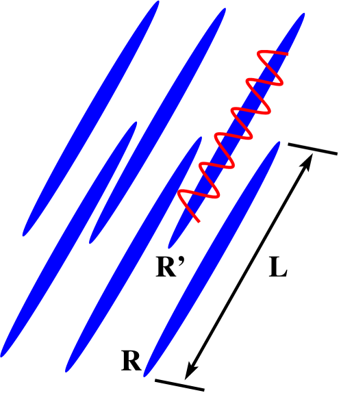
Figure 1: Sketch of a two-dimensional array of coupled tubes (also called quasi-1D optical lattice in this work). Bosons can hop from tube to tube with amplitude $J$, which can be controlled by the height of an optical potential transverse to the tube axis. Along the tube, a periodic optical potential (for clarity, shown here for only one of the tubes) can be also applied. This potential can drive a quantum phase transition where each tube transforms into a 1D Mott insulator.

Taking into account the above considerations, we are led to consider the following Hamiltonian:

$$H=\sum_{\bf R}\int^{L}_{0}dx\>\left[\frac{\hbar^{2}}{2M}\partial_{x}\Psi^{{\dagger}}_{\bf R}(x)\partial_{x}\Psi_{\bf R}(x)+u(x)\rho_{\bf R}(x)+\frac{1}{2}\int^{L}_{0}dx^{\prime}\,v_{a}(x-x^{\prime})\rho_{\bf R}(x)\rho_{\bf R}(x^{\prime})\right]$$

$$-\frac{J}{2}\sum_{\langle{\bf R},{\bf R}^{\prime}\rangle}\int^{L}_{0}dx\left[\Psi^{{\dagger}}_{\bf R}(x)\Psi_{{\bf R}^{\prime}}(x)+{\rm h.c.}\right],$$ (3)

where $\rho_{\bf R}(x)=\Psi^{{\dagger}}_{\bf R}(x)\Psi_{\bf R}(x)$ is the density operator at point $x$ and lattice site $\bf R$; the field operator $\Psi_{\bf R}(x)$ obeys $[\Psi_{\bf R}(x),\Psi_{\bf R^{\prime}}^{{\dagger}}(x^{\prime})]=\delta_{\bf RR^{\prime}}\>\delta(x-x^{\prime})$, and commutes otherwise as corresponds to bosons. The last term in equation (2.1) describes the hopping of bosons between two neighboring tubes. This term is also known as Josephson coupling. The hopping amplitude [28]:

$$J\simeq\frac{4E_{R}}{\sqrt{\pi}}\left(\frac{V_{0\perp}}{E_{R}}\right)^{\frac{3}{4}}\>e^{-2\left(V_{0\perp}/E_{R}\right)^{\frac{1}{2}}},$$ (4)

for $V_{0\perp}\gg E_{R}$. We shall assume a very deep transverse potential so that $J\ll\mu_{1D}$, where $\mu_{1D}=\mu_{1D}(\rho_{0})$ is the chemical potential in each tube, as can be obtained from the exact solution of Lieb and Liniger [1] (or measured experimentally). Since experimentally $\mu_{1D}<0.1\>\hbar\omega_{\perp}$  [7], assuming $J\ll\mu_{1D}$ requires at least that $V_{0\perp}>10\>E_{R}$. Such limit allows us to regard the system as an array of weakly coupled 1D interacting Bose gases.

In the experimental systems, the Mott potential $u(x)$, besides the periodic part described above, also contains a slowly varying harmonic term that confines the atoms longitudinally. Additionally, there are also harmonic traps in the transverse directions. This makes the array, not only finite, but also inhomogeneous. Whereas we shall discuss finite-size effects further below (see section 5), it has proven so far intractable in 1D (except for a few limiting cases [29]) to deal with the harmonic confinement analytically and only numerical results are available [30, 31, 32, 33, 34, 35]. Thus, with the exception of section 7 where we discuss the experimental consequences of our work, we shall neglect the effect of the harmonic potential, and treat the system as an array of gas tubes of length $L$ and hard-wall box (open) boundary conditions [36, 37, 38], each one containing $N_{0}=\rho_{0}L$ bosons (in typical experiments, $N_{0}$ ranges from a few tens to a few thousand particles). This makes sense, however, as much of the interest of this work is focused on computing the phase diagram as well as some of the thermodynamic properties of the different phases, for which one is required to take the thermodynamic limit $L\to\infty$ at constant density $\rho_{0}=N_{0}/L$.

Finally, when the axial potential $u(x)$ is made so deep that $|u_{0}|\gg\mu_{1D}$ (but still $|u_{0}|\ll V_{0\perp}$), it becomes convenient to perform a further projection of $\Psi_{\bf R}(x)$ onto the lowest Bloch band of the Mott potential $u(x)$. Thus,

$$\Psi_{\bf R}(x)\simeq\sum_{m=1}^{M}w_{m}(x)\>b_{m{\bf R}},$$ (5)

where $[b_{m{\bf R}},b_{m^{\prime}{\bf R}}]=\delta_{{\bf R},{\bf R}^{\prime}}\>\delta_{m,m^{\prime}}$, commuting otherwise, and $w_{m}(x)$ is the Wannier orbital centered around site $m$. This projection leads to the so-called Bose-Hubbard model [39]:

$$H_{\rm BH} = \sum_{\bf R}H_{\bf R}+H_{J},$$ (6)

$$H_{\bf R} = -\frac{J_{x}}{2}\sum_{\langle m,m^{\prime}\rangle}b^{\dagger}_{m\bf R}b_{m^{\prime}{\bf R}}+\frac{U}{2}\sum_{m}n^{2}_{m{\bf R}},$$ (7)

$$H_{J} = -\frac{J}{2}\sum_{\langle{\bf R},{\bf R}^{\prime}\rangle,m}\left[b^{{\dagger}}_{m\bf R}b_{m\bf R^{\prime}}+{\rm h.c.}\right],$$ (8)

where $n_{m\bf R}=b^{\dagger}_{m\bf R}b_{m\bf R}$ is the boson number operator at site $(m,{\bf R})$. Note that $|u_{0}|\ll V_{0\perp}$ implies that $J_{x}\gg J$, and therefore we are dealing with a very anisotropic (quasi-1D) version of the Bose-Hubbard model.

2.2 Bosonization and low-energy effective theory

In order to treat the interactions in a non-perturbative way, it is convenient to rewrite (2.1) in terms of collective variables that describe phase and density fluctuations. The method of bosonization [2, 17, 40, 37] allows us to obtain such a description. The description is accurate as long as one is interested in the low-temperature and low-frequency properties of the system. In this subsection we shall briefly outline this method, but we refer the reader to the vast literature on the subject [2, 17, 40, 37] for more technical details.

To study the model of equation (2.1), we use the density-phase representation of the field operator. To leading order,

$$\Psi_{\bf R}(x)=({\cal A}_{B}\rho_{0})^{1/2}\>\exp\left[i\theta_{\bf R}(x)\right],$$ (9)

where is ${\cal A}_{B}$ is a model dependent (i.e. non-universal) prefactor (see below). The density operator,

$$\rho_{\bf R}(x)=\left[\rho_{0}-\frac{1}{\pi}\partial_{x}\phi_{\bf R}(x)\right]\sum_{m=\infty}^{+\infty}e^{2im[\pi\rho_{0}x-\phi_{\bf R}(x)]}.$$ (10)

The fields $\theta_{\bf R}(x)$ and $\phi_{\bf R}(x)$ describe collective fluctuations (phonons) of the phase and the density, respectively . Since the density and the phase are canonically conjugate variables, it is possible to show [37, 17] that $\theta_{\bf R}(x)$ and $\phi_{\bf R}(x)$ obey the commutation relation: $[\phi_{\bf R}(x),\partial_{x^{\prime}}\theta_{\bf R^{\prime}}(x^{\prime})]=i\delta_{\bf RR^{\prime}}\delta(x-x^{\prime})$. Furthermore, it is assumed that $\partial_{x}\phi_{\bf R}(x)$ is small compared to the equilibrium density $\rho_{0}$. Note that this approach does not assume the existence of a condensate and thus properly takes into account the quantum and thermal fluctuations, which are dominant in 1D. Indeed, it is the particle density and not a “condensate” density that appears in the density-phase representation of equations (9,10) (unlike usual mean field approaches). Furthermore, the terms of equation (10) with $m\neq 0$ account for the discrete particle nature of the bosons, which is crucial for obtaining a correct description for the transition from the 1D superfluid phase to the 1D Mott insulator [2, 26, 17, 41, 42].

Using equations (9) and (10), the Hamiltonian in (2.1) becomes

$$H_{\rm eff} = \frac{\hbar v_{s}}{2\pi}\sum_{\bf R}\int^{L}_{0}dx\>\left[K\left(\partial_{x}\theta_{\bf R}(x)\right)^{2}+\frac{1}{K}\left(\partial_{x}\phi_{\bf R}(x)\right)^{2}\right]$$ (11)

$$+\frac{\hbar v_{s}g_{u}}{2\pi a^{2}}\sum_{\bf R}\int^{L}_{0}dx\>\cos\left(2\phi_{\bf R}(x)+\delta\pi x\right)$$

$$-\frac{\hbar v_{s}g_{J}}{2\pi a^{2}}\sum_{\langle{\bf R},{\bf R}^{\prime}\rangle}\int^{L}_{0}dx\>\cos\left(\theta_{\bf R}(x)-\theta_{\bf R^{\prime}}(x)\right),$$

where $\delta=(G-2\pi\rho_{0})/\pi=2(a^{-1}-\rho_{0})$ is the mismatch between the density $\rho_{0}$ and the periodicity of the Mott potential. The two last terms are related to the Mott potential and the Josephson coupling, respectively. We use the following dimensionless couplings to characterize their strength:

$$g_{J}=\frac{2\pi J(\rho_{0}a_{0})^{2}}{\hbar v_{s}\rho_{0}}\>{\cal A}_{B},\quad g_{u}=\frac{2\pi u_{0}(\rho_{0}a_{0})^{2}}{\hbar v_{s}\rho_{0}}$$ (12)

where $a_{0}\approx\hbar v_{s}/\mu_{1D}$ is a short-distance cut-off.

The dimensionless parameter $K$ and the sound velocity $v_{s}$ depend both on the density, $\rho_{0}$, and on the strength of the boson-boson interaction. Indeed, for the Lieb-Liniger model, they depend on a single dimensionless parameter, the gas parameter [1] $\gamma=Mg_{1D}/\hbar^{2}\rho_{0}$. Analytical results for these parameters are only available in the small and large $\gamma$ limit (see ref. [37] for results in the intermediate regime):

$$v_{s}K^{-1} \simeq v_{F}\left[1-8\gamma^{-1}\right]\quad(\gamma\gg 1),$$ (13)

$$v_{s}K^{-1} \simeq v_{F}\gamma/\pi^{2}\quad\quad\quad(\gamma\ll 1),$$ (14)

whereas Galilean invariance fixes the product [2, 37]:

$$v_{s}K=v_{F}=\frac{\hbar\pi\rho_{0}}{M}$$ (15)

Therefore, $1\leq K<+\infty$ for the Lieb-Liniger model, $K=+\infty$ corresponding to free bosons and $K=1$ to the Tonks limit. For the Lieb-Liniger model, the formula [37]:

$${\cal A}_{B}(K)\simeq\left(\frac{K}{\pi}\right)^{\frac{1}{2K}}$$ (16)

provides a reasonably good interpolation (accurate to within $10\%$ of the exact results) for the non-universal prefactor of the field operator.

It is worth stressing that in (11) we have retained only terms which can become dominant at low temperatures. In the language of the rernormalization group (RG) these correspond to marginal or relevant operators. Whenever, for reasons to be given below, any of the terms retained in equation (11) becomes irrelevant in the RG sense, we shall drop it and consider the remaining terms only. We emphasize that the validity of (11) is restricted to energy scales smaller than $\min\{T,\mu_{1D}\}$, and therefore its analysis will allow us to determine the nature of the ground state and low-energy excitations of the system.

Interestingly, the effective Hamiltonian of equation (11) also describes the low energy properties of the anisotropic Bose-Hubbard model of (6). This result can be derived by a lattice version of the bosonization procedure [17], followed by a passage to the continuum limit. However, the relationship of the effective parameters $K$, $v_{s}$, $g_{u}$, and $g_{J}$ to microscopic parameters $J_{x}$, $J$, and $U$ is no longer easy to obtain analytically (except for $U$ small [17] and certain limits in 1D [15]). Thus, in this case $K$, $v_{s}$, $g_{u}$, and $g_{J}$ must be regarded as phenomenological parameters, which must be extracted either from the experiment or from a numerical calculation.

3 Bose-Einstein Condensation

Let us first discuss the phenomenon of Bose-Einstein condensation in anisotropic (quasi-1D) optical lattices. This is the phase transition from a normal Bose gas to a Bose-Einstein condensate (BEC), which exhibits some degree of spatial coherence throughout the lattice. Coherence arises thanks to the Josephson term, which couples the 1D interacting Bose gases together. In the absence of the Josephson coupling and the Mott potential (i.e. for $J=0$ and $u(x)=0$), the system behaves as an array of independent TLL’s [2, 17, 40, 37]: the excitations are 1D sound waves (phonons) and, at zero temperature and for $L\to\infty$, all correlations decay asymptotically as power-laws (e.g. phase correlations $\langle e^{i\theta_{\bf R}(x)}e^{-i\theta_{{\bf R}^{\prime}}(0)}\rangle\sim\delta_{{\bf R},{\bf R}^{\prime}}\>|\rho_{0}x|^{-\frac{1}{2K}}$ for $x\gg\rho^{-1}_{0}$), which implies the absence of long-range order. However, as soon as the Josephson coupling is turned on, bosons can gain kinetic energy in the transverse directions, and therefore become delocalized in more than one tube. This process helps to build phase coherence throughout the lattice and leads to the formation of a BEC. Nevertheless, the building of coherence just described can be suppressed by two kinds of phenomena: one is quantum and thermal fluctuations, which prevent the bosons that hop between different gas tubes from remaining phase coherent. The other is the existence of a Mott potential that is commensurate with the boson density. For sufficient repulsion between the bosons, this leads to the stabilization of a 1D Mott insulator, where bosons become localized. Whereas we shall deal with the latter phenomenon in section 4, we deal with the fluctuations in this section.

In this section we have in mind two different experimental situations: one is a 2D optical lattice where the Mott potential is (experimentally) absent. The other is when the Mott potential is irrelevant in the RG sense. The precise conditions for this to hold will be given in section 4 but, by inspection of (11), we can anticipate that one particular such case is when the Mott potential is incommensurate with the boson density (i.e. $\delta\neq 0$). Under these circumstances, the cosine term proportional to $g_{u}$ oscillates rapidly in space and therefore its effect on the ground state and the long wave-length excitations is averaged out.

3.1 Mean field theory

To reduce the Hamiltonian (2.1) to a tractable problem, we treat the Josephson coupling in a mean-field (MF) approximation where the boson field operator $\Psi_{\bf R}(x)$ is replaced by $\psi_{c}+\delta\Psi_{\bf R}(x)$, where $\psi_{c}=\langle\Psi_{R}(x)\rangle$ and $\delta\Psi_{\bf R}(x)=\Psi_{\bf R}(x)-\psi_{c}$. We then neglect the term $\propto\delta\Psi_{\bf R}(x)\delta\Psi_{\bf R^{\prime}}(x)$, which describes the effect of fluctuations about the mean field state characterized by the order parameter $\psi_{c}$. This approximation decouples the 1D systems at lattice sites $\bf R\neq{\bf R}^{\prime}$ so that the problem reduces to a single “effective” 1D system in the presence of a (Weiss) field proportional to $|\psi_{c}|$. The bosonized form of the Hamiltonian for this system is (we drop the lattice index $\bf R$):

$$H^{\rm MF}_{\rm eff} = \frac{\hbar v_{s}}{2\pi}\int^{L}_{0}\left[K\left(\partial_{x}\theta(x)\right)^{2}+K^{-1}\left(\partial_{x}\phi(x)\right)^{2}\right]$$ (17)

$$-2Jz_{C}\sqrt{{\cal A}_{B}\rho_{0}}|\psi_{c}|\int^{L}_{0}dx\>\cos\theta(x)+Jz_{C}L|\psi_{c}|^{2},$$

where $z_{C}$ is the coordination number of the lattice ($z_{C}=4$ for the square lattices realized thus far in the experiments). The phase of the order parameter $\theta_{c}=\arg\psi_{c}$ has been eliminated by performing a (global) gauge transformation $\theta(x)\to\theta(x)+\theta_{c}$, and henceforth we shall take $\psi_{c}=|\psi_{c}|$ to be real. We note that, up to the last constant term, $H^{\rm MF}_{\rm eff}$ defines an exactly solvable model, the sine-Gordon model, of which a great deal is known from the theory of integrable systems as well as from various approximation schemes [40, 17, 43]. The mean-field Hamiltonian must be supplemented by a self-consistency condition, which relates the effective 1D system to the original lattice problem:

$$\psi_{c}=\langle\Psi_{\bf R}(x)\rangle=2\left({\cal A}_{B}\rho_{0}\right)^{1/2}\,\langle\cos\theta(x)\rangle_{\rm MF}$$ (18)

Note that the average over the cosine must be computed using the eigenstates of $H^{\rm MF}_{\rm eff}$.

3.1.1 Condensate fraction at $T=0$:

To obtain the condensate fraction at zero temperature, we first compute the ground-state energy of $H^{\rm MF}_{\rm eff}$ using the following result for the ground state energy density of the sine-Gordon (sG) model [43]:

$${\cal E}_{sG}(|\psi_{c}|)=-\frac{\Delta_{s}^{2}(|\psi_{c}|)}{4\hbar v_{s}}\tan{\frac{\pi p}{2}},$$ (19)

where $p=\beta^{2}/(8\pi-\beta^{2})=1/(8K-1)$, with $\beta^{2}=\pi/K$. The excitations of the sG model are gapped solitons and anti-solitons (and bound states of them for $\beta^{2}<4\pi$) [40, 17]. The soliton energy gap (also called soliton “mass”) is [43]:

$$\Delta_{s}(|\psi_{c}|)=\hbar v_{s}\left[\frac{m_{s}(|\psi_{c}|)}{\kappa(p)}\right]^{\frac{p+1}{2}},$$ (20)

and

$$m_{s}(|\psi_{c}|) = \frac{z_{C}J({\cal A}_{B}\rho_{0})^{1/2}}{\hbar v_{s}a_{0}^{-2(p+1)/p}}\,|\psi_{c}|,$$ (21)

$$\kappa(p) = \frac{1}{\pi}\frac{\Gamma\left(\frac{p}{p+1}\right)}{\Gamma\left(\frac{1}{p+1}\right)}\left[\frac{\sqrt{\pi}\Gamma\left(\frac{p+1}{2}\right)}{2\Gamma(\frac{p}{2})}\right]^{\frac{2}{p+1}},$$ (22)

where $\Gamma(x)$ is the gamma function. Hence, the ground state energy of $H^{\rm MF}_{\rm eff}$ is given by:

$$E^{\rm MF}_{0}(|\psi_{c}|)/L={\cal E}_{sG}(|\psi_{c}|)+Jz_{C}|\psi_{c}|^{2}.$$ (23)

The self-consistent condition (18) is equivalent to minimizing the mean-field free energy with respect to the order parameter. At $T=0$, the entropy is zero and the condensate fraction is thus obtained by minimizing $E^{\rm MF}_{0}(|\psi_{c}|)$ with respect to $\psi_{c}=|\psi_{c}|$, which yields:

$$\psi_{c}=\rho^{1/2}_{0}\>\left[\frac{p+1}{8(\kappa(p))^{p+1}}\tan\left(\frac{\pi p}{2}\right)\eta^{\frac{p+1}{2}}\left(\frac{Jz_{C}}{\hbar v_{s}\rho_{0}}\right)^{p}\right]^{\frac{1}{1-p}}.$$ (24)

In the above expression, we have introduced the dimensionless parameter $\eta={\cal A}_{B}(K)(\rho_{0}a_{0})^{1/2K}$. We note that the condensate fraction at $T=0$ has a power-law dependence on the amplitude of the Josephson coupling, i.e.

$$\psi_{c}\sim\rho^{1/2}_{0}\left(\frac{J}{\mu_{1D}}\right)^{\frac{p}{1-p}}=\,\rho^{1/2}_{0}\left(\frac{J}{\mu_{1D}}\right)^{\frac{1}{8K-2}}.$$ (25)

The dependence of the exponent on the parameter $K$, which varies continuously with the strength of the interactions between the bosons in the tubes, is a consequence of the fact that the appearance of a BEC at $T=0$, as soon as $J$ is made different from zero, is affected by the characteristic 1D quantum fluctuations of the TLL’s. This behavior is markedly different from what can be obtained by a Gross-Pitaevskii mean-field treatment of the system that overlooks the importance of 1D quantum fluctuations. Further below we shall also encounter other instances where the present results strongly deviate from Gross-Pitaevskii theory.

To show the effectiveness of the fluctuations to cause depletion of the BEC, let us estimate the fraction of bosons in the condensate at $T=0$ using equation (24). For $K=1$ (i.e. the Tonks limit, where phase fluctuations are the strongest), we take $a_{0}\rho_{0}=1$ and assume that $\mu_{1D}=0.1\,\hbar\omega_{\perp}$ [7]. Therefore, for $V_{0\perp}=20\>E_{R}$, the hopping amplitude $J\simeq 3\times 10^{-3}\,\mu_{1D}$, and hence, using equation (24), $\rho^{-1}_{0}\psi^{2}_{c}\approx 20\>\%$. We also note that for weakly interacting bosons, i.e. as $K\to+\infty$, $\psi^{2}_{c}\to\rho_{0}$, as expected.

In the experiments of Ref. [10], very small coherence fractions were observed. The experimental coherence fraction is defined as the fraction of the total number of atoms that contributes to the peak around ${\bf k}=0$ in the momentum distribution, as measured by time of flight. The fraction was quantified by fitting a gaussian distribution to the peak [10]. We note that such a procedure yields a non-vanishing coherence fraction even for the case of uncoupled 1D tubes, where the momentum distribution exhibits a peak with a power-law tail $\sim|k|^{\frac{1}{2K}-1}$ and a width $\sim\max\{L,\hbar v_{s}/T\}$ [37, 36]. Thus, identifying the condensate fraction with the experimental coherence fraction may not be appropriate as there is no condensate in such a 1D limit. Furthermore, as we show below, in the anisotropic BEC phase discussed above, this experimental procedure would also pick up a non-condensate contribution to the coherence fraction. Nevertheless, provided heating effects and thermal depletion of the condensate are not too strong, one can regard the experimental coherence fraction as an upper bound to the condensate fraction, and since a strong decrease of the coherence fraction was reported in the experiments of Ref. [10], our results showing a strong depletion of the condensate are consistent with the experimental findings.

3.1.2 Condensation temperature:

At finite temperatures, thermal (besides quantum) fluctuations cause depletion of the condensate. Ultimately, at a critical temperature $T=T_{c}$, the condensate is destroyed by the fluctuations. To compute the critical temperature we follow Efetov and Larkin [44] and, taking into account that near $T_{c}$ the order parameter $\psi_{c}(T)$ is small, consider a perturbative expansion of the self-consistency condition (18) in powers of $\psi_{c}$. To lowest order,

$$\psi_{c}(T) = \langle\Psi(x,\tau)\rangle_{\rm MF}=\frac{\langle{\cal T}\left\{\Psi(x,\tau)e^{-\frac{1}{\hbar}\int^{\hbar\beta}_{0}d\tau^{\prime}\,H_{\rm W}(\tau^{\prime})}\right\}\rangle_{0}}{\langle{\cal T}e^{-\frac{1}{\hbar}\int^{\hbar\beta}_{0}d\tau^{\prime}\,H_{\rm W}(\tau^{\prime})}\rangle_{0}}$$ (26)

$$= -Jz_{C}\psi_{c}(T)\int^{L}_{0}dx^{\prime}\int^{\hbar\beta}_{0}d\tau^{\prime}g_{1}(x^{\prime},\tau^{\prime})+O(\psi^{2}_{c}).$$

where $\Psi(x,\tau)=(\rho_{0}{\cal A_{B}})^{1/2}\,e^{i\theta(x,\tau)}$, $\tau$ being the imaginary time, ${\cal T}$ the ordering symbol in (imaginary) time, and the Weiss field,

$$H_{\rm W}=-Jz_{C}\psi_{c}(T)\int^{L}_{0}dx\>\left[\Psi(x)+{\rm h.c.}\right].$$ (27)

The correlation function:

$$g_{1}(x,\tau)=-\frac{1}{\hbar}\langle{\cal T}\left[\Psi(x,\tau)\Psi^{{\dagger}}(0,0)\right]\rangle_{0},$$ (28)

where the average $\langle\ldots\rangle_{0}$ is performed using the quadratic part of $H^{\rm MF}_{\rm eff}$. Hence, analytically continuing to real time, equation (26) reduces to:

$$1+Jz_{C}\,g^{R}_{1}(q=0,\omega=0;T_{c})=0,$$ (29)

which determines $T_{c}$; $g^{R}_{1}(q,\omega)$ is Fourier transform of the retarded version of (28). This function is computed in the B (cf. equation (185)), and leads to the result:

$$\left(\frac{2\pi T_{c}}{\hbar v_{s}\rho_{0}}\right)^{2-\frac{1}{2K}}=F(K)\left(\frac{Jz_{C}}{\hbar v_{s}\rho_{0}}\right),$$ (30)

where

$$F(K)=\pi^{2}{\cal A}_{B}(K)\sin\left(\frac{\pi}{4K}\right)B^{2}\left(\frac{1}{8K},1-\frac{1}{4K}\right),$$ (31)

with $B(x,y)=\Gamma(x)\Gamma(y)/\Gamma(x,y)$ the beta function. Thus, the dependence of $T_{c}$ on $J$ is a power-law whose exponent is determined by $K$. It is interesting to analyze the behavior of $T_{c}$ in the limit of weak interactions, i.e. for $K\gg 1$. Using that $F(K\gg 1)\sim K$, along with Galilean invariance, equation (15), $v_{s}=v_{F}/K$, we find that

$$\left(\frac{T_{c}}{\epsilon_{F}}\right)^{2}\sim\left(\frac{J}{\epsilon_{F}}\right),$$ (32)

where $\epsilon_{F}=\hbar\pi\rho_{0}v_{F}/2=(\hbar\pi\rho_{0})^{2}/2M$. Thus, we see that as $K\to+\infty$, $T_{c}\sim J^{1/2}$. This result comes with two caveats. The first one is that, as we turn off the interactions (i.e. for $g_{1D}\to 0$) so that $K$ can diverge, the chemical potential $\mu_{1D}\simeq g_{1D}\rho_{0}\to 0$. Therefore since the effective Hamiltonian, equation (11), is valid only for energy scales below $\mu_{1D}$, the range of validity of the result is going to lower and lower $J$ in this limit. Indeed one cannot simply let $K\to\infty$ and keep $J$ fixed. One would get $T_{c}/\mu_{1D}\sim(\epsilon_{F}/\mu_{1D})^{1/2}(J/\mu_{1D})^{1/2}\to+\infty$. On the other hand, we know that as $g_{1D}\to 0$ $T_{c}$ must remain finite because a non-interacting Bose gas in a 2D optical lattice indeed undergoes Bose-Einstein condensation (see below). Therefore, if $T_{c}/\mu_{1D}$ diverges as $\mu_{1D}\to 0$ for $K\gg 1$, it is because of this fact. The second caveat is that the behavior $T_{c}\sim J^{1/2}$ implied by (32) is not the correct one in the non-interacting limit. To see this, consider the condition for the Bose-Einstein condensation of a non-interacting Bose gas in a 2D optical lattice (we take $L\to\infty$ but keep the number of lattice sites $M_{0}=M_{y}\times M_{z}$ finite):

$$L\sum_{{\bf Q}}\int^{+\infty}_{-\infty}\frac{dq}{2\pi}\,\frac{1}{e^{\left[\epsilon(q)+\epsilon_{\perp}({\bf Q})\right]/T_{c}}-1}=N_{\rm ex}=N_{0}M_{0}$$ (33)

where $\epsilon(q)$ and $\epsilon_{\perp}({\bf Q})=-2J\left(\cos Q_{y}a+\cos Q_{z}a-2\right)$ are the longitudinal and transverse dispersion of the bosons, respectively. In the latter case, we have chosen the zero-point energy (i.e. the bottom of the band) to be zero. In the $J\to 0$ limit the 1D systems become decoupled and $T_{c}$ vanishes (i.e. there is no BEC in 1D). Therefore, we expect $T_{c}$ to be small for small $J$. It is thus justified to expand about ${\bf Q}=(0,0)$ the transverse dispersion $\epsilon_{\perp}({\bf Q})\simeq Ja^{2}{\bf Q}^{2}$. Furthermore, $\epsilon(q)=\hbar^{2}q^{2}/2M$, for free bosons, and thus (33) leads to the law $T_{c}\sim J^{2/3}$, which is different from (32). The difference stems from the assumption of a linear longitudinal dispersion of the excitations implied by the quadratic part of (11) and (17). Had we insisted in assuming a linear longitudinal dispersion of the bosons $\epsilon(q)=\hbar v_{0}|q|$, where $v_{0}$ has dimensions of velocity, we would have found that $T_{c}\sim J^{1/2}$ as implied by (32). This argument implicitly assumes that in the weakly interacting limit, the difference between particles and excitations vanishes. This seems quite reasonable, as the spectrum of excitations of the non-interacting Bose gas coincides with the single-particle spectrum.

Nevertheless, we can expect equation (30) to provide a good estimate of the condensation temperature as long as $J/\mu_{1D}\ll 1$. This is of course particularly true in the strongly interacting limit where $K\sim 1$. The interpolation formula for the prefactor ${\cal A}_{B}$, equation (16), allows to be more quantitative than Efetov and Larkin and to obtain an estimate of $T_{c}$ for $K=2$, for instance. For the Lieb-Liniger model this value of $K$ corresponds to $\gamma\simeq 3.5$ [37] and to $\mu_{1D}/\epsilon_{F}\simeq 0.367$. For $J\simeq 3\times 10^{3}\,\mu_{1D}$ (i.e. $V_{0\perp}=20\,E_{R}$), equation (30) yields $T_{c}/\mu_{1D}\simeq 0.6$ and therefore $T_{c}/\hbar\simeq 10\,{\rm kHz}$ or $T_{c}\simeq 70\,{\rm nK}$. We note this temperature seems to be well above the experimental estimate for the temperature of the cloud, $T<10^{-3}\>\hbar\omega_{\perp}\approx 10^{-2}\mu_{1D}$ [7]. Thus, we expect the experimentally realized systems to be in the anisotropic BEC phase described in this section, and the optical lattice to exhibit 3D coherence.

3.1.3 Excitations of the BEC phase:

Let us next compute the excitation spectrum of the BEC. Due to the existence of coherence between the 1D systems of the array, this turns out to be very different from the “normal” Bose gas (TLL) phase, where the gas tubes are effectively decoupled (i.e. $\psi_{c}=0$) because fluctuations destroy the long range order. The most direct way of finding the excitation spectrum is to consider configurations where the order parameter varies slowly with $x$ and $\bf R$ and time. Thus the order parameter becomes a quantum field, $\Psi_{c}(x.{\bf R},t)$. One then asks what is the effective Lagragian, or Ginzburg-Landau (GL), functional, ${\cal L}_{\rm GL}(x,{\bf R},t)$, that describes the dynamics of $\Psi_{c}(x,{\bf R},t)$. There are at least two ways of finding this functional: one is to perform a Hubbard-Stratonovich transformation and to integrate out the original bosons to find an effective action for the fluctuations of the order parameter about a uniform configuration. To gaussian order (random phase approximation, RPA) this is carried out in  A. This method has the advantage of allowing us to make contact with the microscopic theory (the Hamiltonian (11) in our case) and thus to relate the parameters that determine the dispersion of the excitation modes to those of the microscopic theory. Another method, which we shall follow in this section, is to guess ${\cal L}_{\rm GL}$ using symmetry principles only. To this end, we first write ${\cal L}_{\rm GL}={\cal T}-{\cal V}$, where the kinetic energy term ${\cal T}$ depends on gradients of $\Psi_{c}(x,{\bf R},t)$, whereas ${\cal V}$ depends only on $\Psi_{c}(x,{\bf R},x,t)$. Both ${\cal T}$ and ${\cal V}$ are subject to invariance under global Gauge transformations: $\Psi_{c}(x,{\bf R},t)\to e^{i\theta_{0}}\>\Psi_{c}(x,{\bf R},t)$.

Using global gauge invariance, to the lowest non-trivial order in $\Psi_{c}$, we can write ${\cal V}=a|\Psi_{c}(x,{\bf R},t)|^{2}+b|\Psi_{c}(x,{\bf R},t)|^{4}$. Since we are interested in the ordered phase where $\Psi_{c}=\psi_{c}$, we must have $a<0$. Thus, we can write $\cal V$ as follows:

$${\cal V}=\frac{\hbar\lambda}{2}\left(|\Psi_{c}(x,{\bf R},t)|^{2}-|\psi_{c}|^{2}\right)^{2},$$ (34)

where $\lambda$ is a phenomenological parameter. On the other hand, in order to guess the form of the kinetic term ${\cal T}$ global gauge invariance alone is not sufficient. Further insight can be obtained by close inspection of the effective low-energy theory described by (11). If we write it down in Lagragian form:

$${\cal L}_{\rm eff}(x,t)=\frac{\hbar K}{2\pi}\sum_{\bf R}\left[\frac{1}{v_{s}}\left(\partial_{t}\theta_{\bf R}\right)^{2}-v_{s}\left(\partial_{x}\theta_{\bf R}\right)^{2}\right]+\frac{\hbar v_{s}g_{J}}{2\pi a_{0}^{2}}\sum_{\langle{\bf R},{\bf R^{\prime}}\rangle}\cos\left(\theta_{\bf R}-\theta_{{\bf R^{\prime}}}\right),$$ (35)

we see that it is invariant under Lorentz transformations of the coordinates $(x,t)$ where:

$$\left(\begin{array}[]{c}v_{s}t^{\prime}\\ x^{\prime}\end{array}\right)=\left(\begin{array}[]{cc}\cosh\beta&\sinh\beta\\ \sinh\beta&\cosh\beta\end{array}\right)\left(\begin{array}[]{c}v_{s}t\\ x\end{array}\right),$$ (36)

being $\beta$ a real number. Thus, ${\cal T}$ can only contain Lorentz invariant combinations of $|\partial_{t}\Psi_{c}(x,{\bf R},t)|^{2}$, $|\partial_{x}\Psi_{c}(x,{\bf R},t)|^{2}$, and $|\nabla_{\bf R}\Psi_{c}(x,{\bf R},t)|^{2}$, which are the lowest order derivative terms allowed by global gauge invariance. This leads to

$${\cal T}(x,{\bf R},t)=\frac{\hbar Z_{2}}{2}\left[|\partial_{t}\Psi_{c}(x,{\bf R},t)|^{2}-v^{2}_{||}|\partial_{x}\Psi_{c}(x,{\bf R},t)|^{2}-v^{2}_{\perp}|\nabla_{\bf R}\Psi_{c}(x,{\bf R},t)|^{2}\right],$$ (37)

where $v_{||}=v_{s}$ and $Z_{2}$ and $v_{\perp}$ are again phenomenological parameters. Higher order terms and derivatives are also allowed, but the above terms are the ones that dominate at long wave-lengths and low frequencies. Therefore, the GL functional reads:

$${\cal L}_{\rm GL}(x,{\bf R},t) = \frac{\hbar Z_{2}}{2}\Big{[}|\partial_{t}\Psi_{c}(x,{\bf R},t)|^{2}-v^{2}_{||}|\partial_{x}\Psi_{c}(x,{\bf R},t)|^{2}$$ (38)

$$-v^{2}_{\perp}|\nabla_{\bf R}\Psi_{c}(x,{\bf R},t)|^{2}\Big{]}-\frac{\hbar\lambda}{2}\left(|\Psi_{c}(x,{\bf R},t)|^{2}-|\psi_{c}|^{2}\right)^{2}.$$

We find the excitation spectrum by setting $\Psi_{c}(x,{\bf R},t)=\left[\psi_{c}+\eta_{c}(x,{\bf R},t)\right]\>e^{i\theta_{c}(x,{\bf R},t)}$ and keeping only terms up to quadratic order, which yields:

$${\cal L}_{\rm GL}(x,{\bf R},t) \simeq \frac{\hbar Z_{2}}{2\hbar}\left[\left(\partial_{t}\eta_{c}\right)^{2}-v^{2}_{||}\left(\partial_{x}\eta_{c}\right)^{2}-v^{2}_{\perp}\left(\nabla_{\bf R}\eta_{c}\right)^{2}-Z^{-1}_{2}\lambda\psi^{2}_{c}\eta^{2}_{c}\right]$$ (39)

$$+\frac{\hbar Z_{2}}{2\hbar}\psi^{2}_{c}\left[\left(\partial_{t}\theta_{c}\right)^{2}-v^{2}_{||}\left(\partial_{x}\theta_{c}\right)^{2}-v^{2}_{\perp}\left(\nabla_{\bf R}\theta_{c}\right)^{2}\right]$$

Hence $\omega^{2}_{-}(q,{\bf Q})=(v_{||}q)^{2}+\left(v_{\perp}{\bf Q}\right)^{2}$ gives the dispersion of the Goldstone mode $\theta_{c}$, and $\omega^{2}_{+}(q,{\bf Q})=\Delta^{2}_{+}+(v_{||}q)^{2}+\left(v_{\perp}{\bf Q}\right)^{2}$, where $\Delta^{2}_{+}=Z^{-1}_{2}|\psi_{c}|^{2}\lambda$, the dispersion of the longitudinal mode $\eta_{c}$. Hence we conclude that the BEC phase has two excitation branches: a gapless mode, which is expected from Goldstone’s theorem, and a gapped mode, the longitudinal mode, which describes oscillations of the magnitude of the order parameter about its ground state value $\psi_{c}$. It is worth comparing these phenomenological results with those of the analysis of gaussian fluctuations (RPA + SMA) about the mean-field state described in A. There we find, in the small $(q,{\bf Q})$ limit:

$$\omega^{2}_{-}(q,{\bf Q}) \simeq (v_{||}q)^{2}+(v^{(-)}_{\perp}{\bf Q})^{2},$$ (40)

$$\omega^{2}_{+}(q,{\bf Q}) \simeq \Delta^{2}_{(+)}+(v_{||}q)^{2}+(v^{(+)}_{\perp}{\bf Q})^{2},$$ (41)

where $v^{(-)}_{\perp}=\Delta_{1}a/\hbar$, $\Delta^{2}_{+}=\Delta_{2}(8K-1)^{-2}/2\hbar^{2}$, and $v^{(+)}_{\perp}=\Delta_{2}a/\hbar$, being $\Delta_{p}=\Delta_{s}\sin(p\pi)$ the breather energy gaps and

$$\Delta_{s}=\hbar v_{s}\rho_{0}\left[\eta\frac{p+1}{8\kappa^{2}(p)}\tan\left(\frac{\pi p}{2}\right)\frac{4J}{v_{s}\rho_{0}}\right]^{\frac{1+p}{2(1-p)}}\sim\left(\frac{J}{\mu_{1D}}\right)^{\frac{2K}{4K-1}}.$$ (42)

is the soliton gap. One noticeable difference of these results from those of the GL theory is that the values of $v_{\perp}$ predicted by the RPA+SMA for the longitudinal and Goldstone modes differ, i.e. $v^{(+)}_{\perp}\neq v^{(-)}_{\perp}$. This is due to a poor treatment of the Landau-Ginburg theory that neglected terms of ${\cal L}_{GL}$ of order higher than quadratic in the fields $\eta_{c}$ and $\theta_{c}$. These terms represent interactions between the Goldstone and longitudinal field, as well as self-interactions of the longitudinal field. On the other hand, the RPA treatment of A takes into account some of these interactions and thus yields a correction to the dispersion of the Goldstone and longitudinal modes, which leads to different values of $v_{\perp}$.

It is interesting to consider the behavior of the system in the limit of strong Josephson coupling where $J>\mu_{1D}$. Under these conditions the motion of the atoms is not mainly confined to 1D and thus they can more easily avoid collisions. Therefore, the effect of fluctuations is expected to be less dramatic and assuming the existence of a 3D condensate is a good starting point. This leads to Gross-Pitaevskii (GP) theory, which, assuming a slowly varying configuration of the order parameter, has the following Lagrangian:

$${\cal L}_{\rm GP}(x,{\bf R},t) = \hbar Z_{1}\Big{[}i\Psi^{*}_{c}(x,{\bf R},t)\partial_{t}\Psi_{c}(x,{\bf R},t)-\frac{\hbar}{2M}|\partial_{x}\Psi_{c}(x,{\bf R},t)|^{2}$$ (43)

$$-\frac{y_{\perp}}{2}|\nabla_{\bf R}\Psi_{c}(x,{\bf R},t)|^{2}\Big{]}-\frac{\hbar\lambda}{2}\left(|\Psi_{c}(x,{\bf R},t)|^{2}-|\psi_{c}|^{2}\right)^{2}.$$

where $Z_{1}=a^{-2}$, $y_{\perp}=a^{2}J/\hbar$, and $\lambda=Z_{1}\tilde{g}/\hbar$, $\tilde{g}=4\pi\hbar^{2}a_{s}\int dydz\,|W_{\bf R}(y,z)|^{4}/M$ ($W_{\bf R}(y,z)$ is the Wannier function at site $\bf R$). The condensate fraction $\psi_{c}$ is the solution to the (time-independent) GP equation:

$$\tilde{g}|\psi_{c}|^{2}=z_{C}J+\mu,$$ (44)

where $\mu$ is the chemical potential. Formally, and ignoring the different values of the couplings, ${\cal L}_{GP}$ looks almost identical to ${\cal L}_{GL}$ except for the fact that $i\hbar Z_{1}\Psi^{*}_{c}\partial_{t}\Psi_{c}$ replaces $Z_{2}|\partial_{t}\Psi_{c}|^{2}$. However, this change has a dramatic effect on the excitation spectrum as we show in what follows. Setting $\Psi_{c}(x,{\bf R},t)=\left[\psi_{c}+\eta_{c}(x,{\bf R},t)\right]e^{i\theta_{c}(x,{\bf R},t)}$ and carrying out the same steps as above, we arrive at:

$${\cal L}_{\rm GP}(x,{\bf R},t) = \hbar Z_{1}\Big{[}-2\psi_{c}\eta_{c}\partial_{t}\theta_{c}-\frac{\hbar}{2M}\left(\partial_{x}\eta_{c}\right)^{2}-\frac{y_{\perp}}{2}\left(\nabla_{\bf R}\eta_{c}\right)^{2}-2\lambda\psi^{2}_{c}\eta^{2}_{c}$$ (45)

$$-\frac{\hbar\psi^{2}_{c}}{2M}\left(\partial_{x}\theta_{c}\right)^{2}-\frac{y_{\perp}}{2}\psi^{2}_{c}\left(\nabla_{R}\theta_{c}\right)^{2}\Big{]}.$$

From the above expression, we see that the amplitude $\eta_{c}$ has no dynamics, i.e. there is not term involving $\partial_{t}\eta_{c}$ that is not a total derivative . The term $-2\psi_{c}\eta_{c}\partial_{t}\theta_{c}$, however, couples the dynamics of the phase $\theta_{c}$ and the amplitude $\eta_{c}$. This is very different from the situation with the GL theory encountered above. We can integrate out $\eta_{c}$, e.g. by using the equations of motion for $\eta_{c}$, which yield $\eta_{c}(x,{\bf R},t)=-Z_{1}\partial_{t}\theta_{c}(x,{\bf R},t)/(2\lambda\psi_{c})+$ gradient terms. Thus, the lagrangian becomes:

$${\cal L}_{\rm GP}(x,{\bf R},t)=\frac{Z^{2}_{1}}{\hbar\lambda}\left[\left(\partial_{t}\theta_{c}\right)^{2}-v^{2}_{||}\left(\partial_{x}\theta_{c}\right)^{2}-v^{2}_{\perp}\left(\nabla_{\bf R}\theta_{c}\right)^{2}\right],$$ (46)

being $v^{2}_{||}=\hbar|\psi_{c}|^{2}\lambda/(2MZ_{1})$ and $v^{2}_{\perp}=y_{\perp}\lambda|\psi_{c}|^{2}/(2Z_{1})$. This means that a BEC described by the GP theory has a single low-energy mode, whose dispersion, $\omega(q,{\bf Q})=\sqrt{v^{2}_{||}q^{2}+v^{2}_{\perp}{\bf Q}^{2}}$, vanishes in the long wave-length limit. This is precisely the Goldstone mode, which corresponds to the one that we have already encountered above when analyzing the excitation spectrum of the GL theory that describes the extremely anisotropic limit where $J\ll\mu_{1D}$. The presence of the Goldstone mode as the lowest energy excitation in both theories is a direct consequence of the spontaneous symmetry breaking of global gauge invariance. Thus both kinds of superfluids are adiabatically connected as $J$ is increased. On the other hand, the latter theory also exhibits a mode, the longitudinal mode, that is gapped for $(q,{\bf Q})=(0,{\bf 0})$. However, the fate of the longitudinal mode as $J$ increases is not clear from the above discussion. To gain some insight into this issue, let us reconsider the derivation of the GL Lagrangian in the light of the previous discussion of GP theory. Apparently, the Lorentz invariance discussed above forbids the existence of a term $i\hbar Z_{1}\Psi^{*}_{c}\partial_{t}\Psi_{c}(x,{\bf R},t)$. Nevertheless, we have to remember the emergence of such an invariance in equation (35) is a consequence of the linear dispersion of the TLL modes of the uncoupled tubes. The dispersion is linear for energies $\hbar\omega\ll\mu_{1D}$, but for $J\sim\mu_{1D}$ non-linear corrections must be taken into account. These break the effective Lorentz invariance of (35) and thus a term of the form $i\hbar Z_{1}\Psi^{*}_{c}\partial_{t}\Psi_{c}$ is allowed. Phenomenologically, we can consider a modified GL theory of the form:

$${\cal L}^{\prime}_{\rm GL}(x,{\bf R},t) = i\hbar Z_{1}\Psi^{*}_{c}\partial_{t}\Psi_{c}+\frac{\hbar Z_{2}}{2}\Big{[}|\partial_{t}\Psi_{c}(x,{\bf R},t)|^{2}-v^{2}_{||}|\partial_{x}\Psi_{c}(x,{\bf R},t)|^{2}$$ (47)

$$-v^{2}_{\perp}|\nabla_{\bf R}\Psi_{c}(x,{\bf R},t)|^{2}\Big{]}-\frac{\hbar\lambda}{2}\left(|\Psi_{c}(x,{\bf R},t)|^{2}-\psi^{2}_{c}\right)^{2}.$$

where $Z_{1}$ is very small for $J/\mu_{1D}\ll 1$ but grows with $J$ and should grow large for $J/\mu_{1D}>1$. We can perform the same analysis as above to find the excitation spectrum, which leads to the following quartic equation for the dispersion of the modes:

$$\left[\omega^{2}-\omega^{2}_{+}(q,{\bf Q})\right]\left[\omega^{2}-\omega^{2}_{-}(q,{\bf Q}]\right]+\frac{4Z^{2}_{1}}{Z^{2}_{2}}\omega^{2}=0.$$ (48)

where $\omega^{2}_{\pm}(q,{\bf Q})$ are the dispersion of the Goldstone and longitudinal modes for $Z_{1}=0$, which have been found above. We see that for small $q$ and ${\bf Q}$ there is a solution such that $\omega^{2}=Aq^{2}+B{\bf Q}^{2}$. Furthermore, there is also a gapped mode, for which $\omega^{2}\to\Delta^{2}_{+}+(Z_{1}/Z_{2})^{2}$ as $q$ and $\bf Q)$ tend towards zero. Thus we see that the gap of the longitudinal mode depends on the ratio $Z_{1}/Z_{2}$. For $Z_{1}\ll Z_{2}$, the dispersion of the longitudinal mode is essentially the same as that obtained from the GL theory. However, as $Z_{1}/Z_{2}$ grows with $J$, the gap increases and therefore the exciting the longitudinal mode becomes more costly energetically. At this point is useful to recall that the RPA analysis in A indicates the existence of a continuum of soliton-antisoliton excitations above a threshold $\hbar\omega=2\Delta_{s}$. The stability of the longitudinal mode is ensured if $\Delta_{+}<2\Delta_{s}$, which seems to be the case provided one trusts the single-mode approximation employed to estimate $\Delta_{+}$. However, as the gap is pushed up towards higher energies by an increasing $Z_{1}/Z_{2}$, the longitudinal mode is likely to acquire a large finite lifetime by coupling to this continuum. This will eventually lead to its disappearance from the spectrum.

3.2 Self-consistent harmonic approximation (SCHA)

An alternative approach to obtain the properties of the BEC phase is the self-consistent Harmonic approximation (SCHA) (see e.g. Ref. [17]). The idea behind this approximation is to find an optimal (in the sense to be specified below) quadratic Hamiltonian that approximates the actual Hamiltonian of the system. The method is more suitably formulated in the path-integral language, where the role of the Hamiltonian is played by the euclidean action. The latter is obtained by performing, in the Lagrangian of equation (35), a Wick rotation to imaginary time, $t\to-i\tau$, and defining the action as $S=-\int^{L}_{0}dx\int^{\hbar\beta}_{0}d\tau\,{\cal L}_{\rm eff}(x,i\tau)/\hbar$. Hence, $S[\theta]=S_{0}[\theta]+S_{J}[\theta]$, where

$$S_{0}[\theta] = \frac{K}{2\pi}\sum_{\bf R}\int_{0}^{L}dx\int_{0}^{\beta}d\tau\left[\frac{1}{v_{s}}\left(\partial_{\tau}\theta_{\bf R}(x,\tau)\right)^{2}+v_{s}\left(\partial_{x}\theta_{\bf R}(x,\tau)\right)^{2}\right],$$ (49)

$$S_{J}[\theta] = -\frac{1}{\hbar}{\cal A}_{B}\rho_{0}J\,\sum_{\langle{\bf RR^{\prime}}\rangle}\int^{L}_{0}dx\int^{\hbar\beta}_{0}d\tau\,\cos(\theta_{\bf R}(x,\tau)-\theta_{\bf R^{\prime}}(x,\tau)).$$ (50)

The partition function reads:

$$Z=\int\left[d\theta\right]\,e^{-S[\theta]}.$$ (51)

In the SCHA, $S[\theta]$ is approximated by a gaussian (i.e. quadratic) action:

$$S_{\rm v}[\theta]=\frac{1}{2M_{0}\hbar\beta L}\sum_{q,{\bf Q},\omega_{n}}G^{-1}_{\rm v}(q,{\bf Q},\omega_{n})\left|\theta_{\bf Q}(q,\omega_{n})\right|^{2},$$ (52)

where $\theta_{\bf Q}(q,\omega_{n})$ is the Fourier transform of $\theta_{\bf R}(x,\tau)$. This gaussian form is motivated by considering the action, equation (50), in the limit of large $J$. We then expect that the replacement $\cos\left(\theta_{\bf R}-\theta_{\bf R^{\prime}}\right)\simeq 1-\frac{1}{2!}\left(\theta_{\bf R}-\theta_{\bf R^{\prime}}\right)^{2}$ would be reasonable. This yields a quadratic action and a phonon propagator the form of (58). To find the optimal $G_{\rm v}(q,{\bf Q},\omega_{n})$, we use Feynman’s variational principle [45]:

$$F=-\frac{1}{\beta}\ln Z\leq F^{\prime}[G_{\rm v}]=F_{\rm v}-\langle\left(S[\theta]-S_{\rm v}[\theta]\right)\rangle_{\rm v},$$ (53)

where $\langle\ldots\rangle_{\rm v}$ stands for the trace over configurations of $\theta_{\bf R}(x,\tau)$ using $e^{-S_{\rm v}[\theta]}$ and

$$e^{-\beta F_{\rm v}}=\int\left[d\theta\right]\,e^{-S_{\rm v}[\theta]}.$$ (54)

Therefore, by extremizing $F^{\prime}[G_{\rm v}]$ with respect to $G_{\rm v}$, that is, by solving

$$\frac{\delta F^{\prime}[G_{\rm v}]}{\delta G_{\rm v}(q,{\bf Q},\omega_{n})}=0,$$ (55)

we find the optimal $G_{\rm v}$:

$$\frac{1}{G_{\rm v}(q,{\bf Q},\omega_{n})}=\frac{1}{G_{0}(q,\omega_{n})}-\frac{{z_{C}\cal A}_{B}(K)\rho_{0}}{2\hbar}Ja^{2}\,F({\bf Q})\,\,e^{\frac{Ja^{2}}{2M_{0}L\hbar\beta}\sum_{q^{\prime},{\bf Q^{\prime}},\omega_{n}^{\prime}}F({\bf Q^{\prime}})\>G_{\rm v}(q^{\prime},{\bf Q^{\prime}},\omega_{n}^{\prime})},$$ (56)

where $F({\bf Q})=\frac{a^{-2}}{2}\sum_{\bf t}\left(1-e^{i{\bf Q}\cdot{\bf t}}\right)$, with $\bf t$ the vectors that connect a lattice point to its nearest neighbors, and $G^{-1}_{0}(q,\omega_{n})=\frac{K}{\pi v_{||}}\left[\omega^{2}_{n}+v^{2}_{||}q^{2}\right]$ the free phonon propagator ($v_{||}=v_{s}$). This self-consistency equation (56) can be solved by rewriting it into two equations as follows: defining

$$v^{2}_{\perp}=\frac{\pi z_{C}{\cal A}_{B}}{2K}(\rho_{0}a)\left(\frac{Ja}{\hbar}\right)v_{||}\>\exp\left[\frac{2a^{2}}{z_{C}M_{0}L\hbar\beta}\sum_{q,{\bf Q},\omega_{n}}F({\bf Q})\>G_{\rm v}(q,{\bf Q},\omega_{n})\right],$$ (57)

we arrive at:

$$G^{-1}_{\rm v}(q,{\bf Q},\omega_{n})=\frac{K}{\pi v_{||}}\left[\omega^{2}_{n}+(v_{||}q)^{2}+v^{2}_{\perp}\,F({\bf Q})\right].$$ (58)

The set of equations (57) and (58) are solved in C), for the variational parameter $v_{\perp}^{2}$ which is the transverse phonon velocity of the 3D superfluid.

At $T=0$, the equation for $v^{0}_{\perp}=v_{\perp}(T=0)$ can be solved analytically. We merely state here the result (the details of the calculation can be found in C):

$$\frac{v^{0}_{\perp}}{v_{||}}\simeq\left[\left(\frac{{\cal B}_{0}{\cal A}_{B}(K)}{K}\right)\left(\frac{\hbar v_{||}\rho_{0}}{\mu_{1D}}\right)\left(\frac{z_{C}J}{\mu_{1D}}\right)\right]^{\frac{2K}{4K-1}}$$ (59)

where ${\cal B}_{0}\simeq 1.2971$ for a 2D square latttice. Note that the variational propagator $G_{\rm v}(\omega_{n},q,{\bf Q})$ has a pole, which for small $q$ and ${\bf Q}$, is located at $\omega^{2}_{-}(q,\omega)\simeq v^{2}_{||}q^{2}+(v_{\perp}{\bf Q})^{2}$, for a square 2D transverse lattice. This is the Goldstone mode with $v_{\perp}\sim(J/\mu_{1D})^{2K/(4K-1)}$, a power law with an exponent that agrees with the RPA+SMA result of A, where it is shown that $v^{(-)}_{\perp}\sim\Delta_{1}\sim\Delta_{s}\sim(J/\mu_{1D})^{2K/(4K-1)}$. However, the SCHA fails to capture the existence of the longitudinal mode. This is because, as described above, the SCHA is tantamount to expanding the cosine in the Josephson coupling term. Such an approximation neglects the fact that the phase $\theta_{\bf R}(x,\tau)$ is $2\pi$-periodic, and that as a consequence the system supports vortex excitations. On the other hand, this is captured by RPA because it does not disregard the periodic aspect of the phase since the mean-field state is described by the sine-Gordon model. The latter has soliton, anti-soliton, and breather excitations, which are a direct consequence of the periodicity of $\theta_{\bf R}$.

In the weakly interacting limit (i.e. for $K\gg 1$), equation (59) becomes:

$$\frac{v^{0}_{\perp}}{v_{||}}\sim\sqrt{\frac{J}{\mu_{1D}}},$$ (60)

where we have used that $\mu_{1D}/(v_{||}\rho_{0})\approx\gamma^{1/2}=\pi/K$ for $K\gg 1$. Thus, the requirement that $J/\mu_{1D}\ll 1$ automatically implies that $v^{0}_{\perp}/v_{||}\ll 1$, that is, we deal with a very anisotropic BEC.

At $T>0$, the variational equations must solved numerically (see C). The absence of a solution to equation (57) such that for $T>T_{c}$ $v_{\perp}=0$ allows us to also determine the condensation temperature. Thus for weakly interacting Bose gas ($K\gg 1$ or $\gamma$ small), we find:

$$\frac{T_{c}}{\mu_{1D}}\simeq\sqrt{\frac{z_{C}J}{\mu_{1D}}}\left(0.610+0.698K\right),$$ (61)

This is the same form as that obtained for large $K$ from the RPA analysis of section 3.1.2, equation (32). Thus, the same caveats as those discussed there apply to it.

At $T=T_{c}$ the velocity $v_{\perp}=v^{c}_{\perp}$ has finite a jump, which for $K\gg 1$ is given by

$$\frac{v^{c}_{\perp}}{v_{\perp}^{0}}\simeq\sqrt{\frac{z_{C}J}{\mu_{1D}}}\left(0.376+0.274K^{-1}\right).$$ (62)

This is indeed an artifact of the SCHA, which incorrectly captures the second-order character of the transition from the BEC to the “normal” (TLL) phase.

3.3 Momentum distribution function

Besides the excitation spectrum, the SCHA also allows us to obtain the momentum distribution of the system in the BEC phase. The latter can be measured in a time-of-flight experiment [25], and it is the Fourier transform of the one-body density matrix:

$$n(k,{\bf K})=\frac{1}{M_{0}L}\int dxdx^{\prime}\,\int d{\bf r}_{\perp}d{\bf r}^{\prime}_{\perp}\,e^{-i{\bf K}\cdot({\bf r}_{\perp}-{\bf r^{\prime}}_{\perp})}\>e^{-ik(x-x^{\prime})}\>\langle\Psi^{{\dagger}}(x,{\bf r}_{\perp})\Psi(x^{\prime},{\bf r}^{\prime}_{\perp})\rangle.$$ (63)

Introducing $\Psi(x,{\bf r}_{\perp})=\sum_{\bf R}W_{\bf R}({\bf r}_{\perp})\>\Psi_{\bf R}(x)$, where ${\bf r}_{\perp}=(y,z)$, $n(k,{\bf K})$ can be written as:

$$n(k,{\bf K})=\frac{|W({\bf K})|^{2}}{M_{0}L}\sum_{{\bf R},{\bf R^{\prime}}}e^{-i{\bf K}\cdot({\bf R}-{\bf R}^{\prime})}\int dxdx^{\prime}\,e^{-ik(x-x^{\prime})}\>\langle\Psi^{{\dagger}}_{\bf R}(x)\Psi_{\bf R^{\prime}}(x^{\prime})\rangle,$$ (64)

where $W({\bf K})$ is the Fourier transform of the Wannier orbital $W_{\bf 0}({\bf r}_{\perp})$. Using the bosonization formula (9) and within the SCHA

$$\langle\Psi^{{\dagger}}_{\bf R}(x)\Psi_{\bf 0}(0)\rangle=\rho_{0}{\cal A}_{\bf B}(K)\langle e^{-i\left[\theta_{\bf R}(x)-\theta_{\bf 0}(0)\right]}\rangle\simeq\rho_{0}{\cal A}_{\bf B}(K)e^{-\frac{1}{2}\langle\left[\theta_{\bf R}(x)-\theta_{\bf 0}(0)\right]^{2}\rangle_{\rm SCHA}}.$$ (65)

Since $\frac{1}{2}\langle\left[\theta_{\bf R}(x)-\theta_{\bf 0}(0)\right]^{2}\rangle_{\rm SCHA}=\langle\theta^{2}_{\bf 0}(0)\rangle_{\rm SCHA}-\langle\theta_{\bf R}(x)\theta_{\bf 0}(0)\rangle_{\rm SCHA}$ and $\langle\theta_{\bf R}(x)\theta_{\bf 0}(0)\rangle=G_{\rm v}(x,{\bf R},t=0)$, where

$$G_{\rm v}(x,{\bf R},t) = \frac{1}{M_{0}L}\sum_{q,{\bf Q}}\int\frac{d\omega}{2\pi}\>e^{i(qx+{\bf Q}\cdot{\bf R}-\omega t)}G_{\rm v}(q,{\bf Q},i\omega_{n}\to\omega+i\delta)$$ (66)

$$\simeq \frac{1}{8\pi^{2}v^{2}_{\perp}K}\frac{a^{2}}{(x/v_{||})^{2}+({\bf R}/v_{\perp})^{2}},$$ (67)

where $G_{\rm v}(q,{\bf Q},\omega_{n})$ is given by equation (58). The result on the last line is the asymptotic behavior for large $x$ and ${\bf R}$. Thus we see that for large distances $G_{\rm v}(x,{\bf R},t)$ decays very rapidly and therefore it is justified to expand $e^{G_{\rm v}(x,{\bf R},t=0)}\simeq 1+G_{\rm v}(x,{\bf R},t=0)+\ldots$ Keeping only the lowest order term, we obtain the following expression for $(k,{\bf K})$ near zero momentum:

$$n(k,{\bf K})\simeq|W({\bf K})|^{2}\>\left[(M_{0}L)|\psi_{c}|^{2}\delta_{k,0}\>\delta_{{\bf K},{\bf 0}}+\frac{v_{||}{\cal Z}_{0}}{\sqrt{(v_{||}k)^{2}+(v_{\perp}{\bf K})^{2}}}\right]$$ (68)

where ${\cal Z}_{0}=|\psi_{c}|^{2}\pi/2K$, and the (modulus squared of the) condensate fraction,

$$|\psi_{c}|^{2}=\rho_{0}{\cal A}_{B}(K)\,e^{-G_{\rm v}(x=0,{\bf R}={\bf 0})}=\rho_{0}{\cal A}_{B}(K)\left(\frac{\hbar v_{\perp}e^{-{\cal C}_{0}}}{2\mu_{1D}a}\right)^{1/2K}\sim\rho_{0}\left(\frac{J}{\mu_{1D}}\right)^{\frac{1}{4K-1}},$$ (69)

where ${\cal C}_{0}\simeq 0.2365$ for a 2D square lattice. Thus the SCHA approximation also yields a condensate fraction that behaves as a power law of $J/\mu_{1D}$. The exponent is the same as the one obtained in section 3.1.1 from mean-field theory, equation (25).

The momentum distribution can be also obtained at finite temperatures from:

$$G_{\rm v}(k,{\bf K},t=0) = \frac{1}{\hbar\beta}\sum_{i\omega_{n}}\frac{\pi v_{||}K^{-1}}{\omega^{2}_{n}+(v_{||}k)^{2}+v^{2}_{\perp}F({\bf K})}$$ (70)

$$= \frac{\pi v_{||}K^{-1}}{\sqrt{(v_{||}q)^{2}+v^{2}_{\perp}F({\bf K})}}\coth\left[\frac{\hbar\sqrt{(v_{||}k)^{2}+v^{2}_{\perp}F({\bf K})}}{T}\right].$$ (71)

Thus for $k$ and $\bf K$ near zero, and $T>0$ we find

$$n(k,{\bf K})\simeq|W({\bf K})|^{2}\>\left[(M_{0}L)|\psi_{c}(T)|^{2}\delta_{k,0}\>\delta_{{\bf K},{\bf 0}}+\frac{Tv_{||}{\cal Z}_{0}(T)/\hbar}{(v_{||}k)^{2}+(v_{\perp}{\bf K})^{2}}\right]$$ (72)

with ${\cal Z}_{0}(T)$ defined as above with $\phi_{c}$ replaced by $\psi_{c}(T)$.

There are several points that are worth discussion about the results of equations (68) and (72). The first is that these form are anisotropic generalizations of the result that can be obtained from Bogoliubov theory for a BEC [25]. However, for sufficiently large $q$ we expect a crossover to the same power-law behavior of a single 1D Bose-gas $\sim|k|^{\frac{1}{2K}-1}$ (for $T=0$ and $L\to\infty$). This is nothing but a reflection of the dimensional crossover physics: bosons with kinetic energy $\epsilon(k)=\hbar^{2}k^{2}/2M\gg J$ (but such that $\epsilon(k)\ll\mu_{1D}$ for the bosonization to remain valid) cannot “feel” the BEC and the intertube coherence. However, they still “feel” the characteristic quantum fluctuations of the TLL state. The second observation is related to our discussion of section 3.1.1 on the experimental “coherence fraction”: it is clear by fitting a gaussian to $n(k,{\bf K})$ about zero momentum, one does not only pick a contribution from $|\psi_{c}(T)|^{2}$ but also from the tail of the non-condensate fraction. The presence of a trap (and the inhomogeneity of the system caused it) should not dramatically modify this conclusion. However, as both contributions are positive, we expect that the experimentally measured coherence fraction is indeed an upper bound for $|\psi_{c}(T)|^{2}$.

4 Deconfinement

In this section we shall obtain the phase diagram of the system for the case where the Mott potential is relevant. One necessary condition for this is that $\delta=0$ and $u_{0}\neq 0$ so that $g_{u}\neq 0$ in equation (11). As it has been mentioned above, under these conditions, and provided repulsion between the bosons is strong enough so that the parameter $K<2$, the system undergoes a transition to a Mott insulating state for $J=0$ and arbitrarily small $u_{0}$ [2, 26, 17, 41]. In the Mott insulating state bosons are localized about the minima of the potential. The question thus is what happens as soon as a small Josephson coupling between neighboring tubes is present. The latter favors delocalization of the bosons leading to the appearance of a BEC, and therefore competes with the localization tendencies favored by the Mott potential. The competition between these two opposite tendencies leads to a new quantum phase transition known as deconfinement. For small values of $|u_{0}|$ and $J$, it can be studied by means of the renormalization group (RG). This is a much better approach than comparing ground state energies of mean-field theories for each phase, as it takes into account the fluctuations, which are entirely disregarded within any mean-field approximation. However, although the RG approach allows us to estimate the position of the boundaries between the Mott insulating and BEC phases, in the present case it cannot provide any insight into the nature of the deconfinement transition. For this, we shall rely on the mean-field approximation and map the mean field hamiltonian at the special value of $K=1/2$ to a spin-chain model.

4.1 Renormalization Group calculation

Let us return to the low-energy effective field theory defined by the Hamiltonian in equation (11). Since it is a description valid for low-energies and temperatures, the couplings $K$, $g_{u}$, $g_{J}$, etc. all depend on the cut-off energy scale, which is typically set by the temperature for $\Lambda=T<\mu_{1D}$. Thus, as the temperature is decreased, the couplings get renormalized due to virtual transitions to states with energy $>\Lambda=T$, which now are excluded from the description. The nature of the ground state is thus determined by the dominant coupling as $T=\Lambda\to 0$.

The change (‘flow’) for the couplings can be described by a set of differential equations. For small values of $g_{J}$ and $g_{u}$ the RG flow equations can be obtained perturbatively to second order in the couplings. The details of such a calculation are given in D. The result reads:

$$\frac{dg_{F}}{d\ell} = \frac{g^{2}_{J}}{K},$$ (73)

$$\frac{dg_{J}}{d\ell} = \left(2-\frac{1}{2K}\right)g_{J}+\frac{g_{J}g_{F}}{2K},$$ (74)

$$\frac{dg_{u}}{d\ell} = \left(2-K\right)g_{u},$$ (75)

$$\frac{dK}{d\ell} = 4g^{2}_{J}-g^{2}_{u}K^{2},$$ (76)

where $\ell\approx\ln\mu/T$. The coupling $g_{F}$ is generated by the RG and describes an interaction between bosons in neighboring tubes. However, since initially there is not such an interaction (i.e. $g_{F}(0)=0$) and as $dg_{F}/d\ell=O(g^{2}_{J})$ its effect on the flow of the other couplings is not very important.

The phase boundary between the BEC and 1D Mott insulator phases can be obtained by studying the asymptotic behavior of the solutions of equations (73) to (76). As the temperature is lowered, i.e. as $\ell\to+\infty$, in the regime $\frac{1}{4}\leq K<2$  the effective couplings $g_{u}(\ell)$ and $g_{J}(\ell)$ grow as both the Mott potential and the Josephson coupling are relevant perturbations in the RG sense. If $g_{u}(\ell)$ grows larger, the localization tendencies of the Mott insulator phase set in, whereas if $g_{J}(\ell)$ grows larger, delocalization tendencies of the BEC phase described in section 3 dominate in the ground state. Both phases correspond to two different strong coupling fixed points of the RG. When both perturbations are relevant, one has a crossing of the two strong coupling fixed points, and since we obtained the above equations assuming that both $g_{u}$ and $g_{J}$ are small, the RG is not perturbatively controlled when $g_{u}$ and $g_{J}$ grow large. Note that, given this limitation, we cannot entirely exclude that intermediate phases might exist. We will come back to that particular point in the next section.

The relative magnitude of the initial (i.e. bare) values of $g_{J}$ and $g_{u}$ determines which coupling grows faster to a value of order one, where the above RG equations cease to be valid. The faster growth of one coupling inhibits the other’s growth via the renormalization of the parameter $K$: If $g_{u}(\ell)$ grows faster, $K$ flows towards $0$, leading to the 1D Mott insulator. This reflects the fact that, for large enough $g_{u}$, the Mott potential drives the system towards an incompressible phase, where boson number fluctuations are strongly suppressed by the localization of the particles. On the other hand, if $g_{J}(\ell)$ grows faster, $K$ also grows and leads to the 3D BEC phase. A rather crude estimate of the boundary can be obtained by ignoring the renormalization of $K$. In such a case, dividing (74) by (75), keeping only the leading order terms, and integrating this equation up to the scale $\ell^{*}$, where both $g_{J}(\ell^{*})=g_{u}(\ell^{*})=s$, where $s\sim 1$ we get that the critical value of $g^{c}_{J}=g_{J}(0)$ for a given value of $g_{u}(0)$ scales as:

$$g^{c}_{J}\sim g_{u}(0)^{\frac{2-1/2K}{2-K}}.$$ (77)

In the next section we will see that this power-law is also recovered in the mean-field treatment of the following section. However, for a more precise estimate of the boundary one needs to integrate numerically the RG-flow equations and take into account the renormalization of $K$, which can be important especially near $K=2$. This is shown in figure 2, where we compare the estimate of (77) with the phase boundary obtained from a numerical integration of the RG equations.

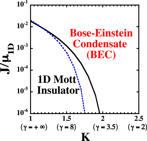
Figure 2: Zero-temperature phase diagram of a 2D array of coupled, infinite, 1D interacting boson systems. The values on the vertical axis are defined up to a factor of order unity. $K$ is the Luttinger-liquid parameter (see section 2.2 for explanations). The corresponding values of Lieb-Liniger gas parameter $\gamma=Mg/\hbar^{2}\rho_{0}$ are also displayed. A longitudinal commensurate optical potential of amplitude $u_{0}$ ($u_{0}\approx 0.03\>\mu_{1D}$ for $K=1$ and $u_{0}\approx 0.02\>\mu$ for $K=2.5$) is assumed. The dashed line corresponds to the crude estimate for the phase boundary obtained from equation (77).

The RG equations also allow to extract the gap of the Mott insulator as well as the soliton energy gap that characterizes the decay of the one-body correlation functions (i.e. the healing length) in the BEC phase. This is achieved by integrating the equations until the fastest grown coupling is of order one. One can then use that, at this scale $\ell^{*}$, the gap $\Delta(\ell)$ is also of order one, and since gaps renormalize like energies, i.e. $\Delta(\ell)=\Delta(\ell=0)e^{-\ell}$. For example, in the BEC phase, using equation (74), keeping only the leading term, and integrating this equation up to a scale $\ell^{*}\approx\log(\Lambda/\Delta_{s})$ where $g_{J}(\ell^{*})\sim 1$ gives $\Delta_{s}\sim(J/\mu_{1D})^{1/(2-1/2K)}$, which has the same power-law behavior as the one obtained from the mean-field theory, equation(42). For $\frac{1}{4}<K<2$, a better estimate (numerical) can be obtained by accounting for the renormalization of $K$ using the full set of RG equations. However, for $K>2$, the renormalization of $K$ is negligible and the previous estimate of $\Delta_{s}$ should be accurate.

Another instance where it can be necessary to take into account the renormalization of $K$ is the evaluation of the condensation temperature $T_{c}$ in the presence of the Mott potential. In particular, for $K<2$, although the initial conditions are such that the coupling $g_{J}$ is the dominant one, $K$ may undergo an important renormalization if $g_{u}$ is non-zero. The renormalized value of $K$ could be then used in combination with the RPA formula, equation (30), for $T_{c}$.

4.2 Mean field theory of the deconfinement transition

The RG approach explained above does not provide any insight into the nature of the deconfinement transition, e.g. it cannot answer questions such as whether the transition is continuous (i.e. second order) or not, or what universality class it belongs to. In order to address, at least partially, some of these issues we will treat again the interchain coupling in a mean field approximation. We begin by rewriting the mean-field Hamiltonian of equation (17) in the presence of the Mott potential:

$$H^{\rm MF}_{\rm eff} = \frac{\hbar v_{s}}{2\pi}\int^{L}_{0}\left[K\left(\partial_{x}\theta(x)\right)^{2}+K^{-1}\left(\partial_{x}\phi(x)\right)^{2}\right]$$ (78)

$$+2\rho_{0}u_{0}\int^{L}_{0}dx\,\cos 2\phi(x)-2Jz_{C}\sqrt{{\cal A}_{B}\rho_{0}}|\psi_{c}|\int^{L}_{0}dx\>\cos\theta(x)+Jz_{C}L|\psi_{c}|^{2}.$$

The new mean-field Hamiltonian is now a double sine-Gordon theory, which is not exactly solvable for general values of the parameter $K$ [46]. However, for $K=\frac{1}{2}$ the solution takes a particularly simple form as one can directly relate it to the results obtained in section 3.1 for the sine-Gordon model. As it has been pointed out above, the regime $K<1$ is not physical for models like the Lieb-Liniger model or the 1D Bose-Hubbard model. However, we expect that the solution at this point captures some of the essential features of the deconfinement transition for $K\geq 1$. Indeed in particular in the RG flow nothing special occurs at $K=1$ so we can expect the two limits to be smoothly connected. The key observation behind the solution at $K=\frac{1}{2}$ is that, as shown in E, at this point (78) is the effective low-energy description of a Heisenberg anti-ferromagnetic spin chain in the presence of a staggered magnetic field:

$$H^{MF}=J_{0}\sum_{m}{\bf S}_{m}\cdot{\bf S}_{m+1}+{\bf h}\cdot\sum_{m}(-1)^{m}\>{\bf S}_{m}+Jz_{C}L|\psi_{c}|^{2},$$ (79)

where ${\bf h}=(h_{x},0,h_{z})$, $h_{x}=-\sqrt{8\pi}z_{C}({\cal A}_{B}\rho_{0})^{1/2}|\psi_{c}|a_{0}J$ and $h_{z}=2\pi u_{0}(\rho_{0}a_{0})$, where $a_{0}$ is the short-distance cut-off. We can perform a rotation about the OY axis, so that the spin variables transform as:

$$S^{x}_{m} = \cos\varphi\>\tilde{S}^{x}_{m}+\sin\varphi\>\tilde{S}^{z}_{m},$$ (80)

$$S^{z}_{m} = -\sin\varphi\>\tilde{S}^{x}_{m}+\cos\varphi\>\tilde{S}^{z}_{m},$$ (81)

where $\tan\varphi=h_{z}/h_{x}$, and the mean-field Hamiltonian becomes:

$$H^{MF}=J_{0}\sum_{m}{\bf\tilde{S}}_{m}\cdot{\bf\tilde{S}}_{m+1}+|{\bf h}|\sum_{m}(-1)^{m}\tilde{S}^{x}_{m}+Jz_{C}L|\psi_{c}|^{2}.$$ (82)

Applying the the spins ${\bf\tilde{S}}_{m}$, the bosonization rules the spins given in E, the above Hamiltonian becomes:

$$H^{\rm MF}_{\rm eff} = \frac{\hbar v_{s}}{2\pi}\int^{L}_{0}\left[\frac{1}{2}\left(\partial_{x}\theta(x)\right)^{2}+2\left(\partial_{x}\phi(x)\right)^{2}\right]$$ (83)

$$+\frac{|{\bf h}|}{a_{0}\sqrt{2\pi}}\int^{L}_{0}dx\>\cos\theta(x)+Jz_{C}L|\psi_{c}|^{2}.$$

This is another sG model, similar to the one that we encountered in section 3.1. One can again make use of equations (19, 20) and (21) to obtain the ground-state energy density,

$$E^{\rm MF}_{0}/L={\cal E}_{sG}(|{\bf h}|)+z_{C}J|\psi_{c}|^{2}.$$ (84)

The behavior of the order parameter $\psi_{c}$ follows from the extremum condition:

$$\frac{d}{d\psi_{c}}\left[{\cal E}_{sG}(|{\bf h}|)+z_{C}J|\psi_{c}|^{2}\right]=0.$$ (85)

The algebra is essentially very similar to that in section 3.1.1, and we just quote the results here. There exists a critical tunneling $J_{c}$, when the condensate fraction $\psi_{c}\rightarrow 0$, i.e. $h_{x}\rightarrow 0$. We find at $K=1/2$,

$$\left(\frac{z_{C}J_{c}}{v_{||}\rho_{0}}\right)^{3}=\frac{\pi\rho_{0}a_{0}[\kappa(1/3)]^{4}}{2[\frac{1}{6}\eta\tan(\pi/6)]^{3}}\left(\frac{u_{0}}{v_{||}\rho_{0}}\right)^{2}.$$ (86)

Thus the condensate fraction grows continuously from zero at the deconfinement transition from the Mott Insulator at $J<J_{c}$ to the 3D anisotropic superfluid at $J>J_{c}$ according to:

$$\psi_{c}^{2}=\rho_{0}\frac{\eta^{2}}{[\kappa(1/3)]^{4}}\left[\frac{1}{6}\tan\left(\frac{\pi}{6}\right)\right]^{3}\left(\frac{z_{C}J}{v_{||}\rho_{0}}\right)\left[1-\left(\frac{J_{c}}{J}\right)^{3}\right],$$ (87)

where $\kappa(1/3)$ has been defined in (22) and at $K=1/2$ the dimensionless ratio $\eta=\rho_{0}a_{0}{\cal A}_{B}(1/2)$. Note that the scaling $J_{c}\propto u_{0}^{2/3}$ in (86) agrees with that deduced from the RG approach of equation (77) upon setting $K=1/2$.

It is instructive to compare this deconfinement scenario in 3D with the case where only two 1D systems are coupled together (via the same Josephson coupling term), i.e. a bosonic two-leg ladder, which has been studied in [47]. In both the quasi-1D optical lattice and the ladder, there is the competition between the Josephson coupling that favors superfluidity, and the localizing tendency of the commensurate periodic potential on top of which the interacting bosons hop. This is manifested in a very similar structure of the bosonized Hamiltonians. For the ladder case, it is convenient use a symmetric and anti-symmetric combination of the fields of the two chains, which leads to slightly different forms for the RG equations. Nevertheless, the mentioned competition occurs for the same range of $K$: $1/4<K<2$, where, in the ladder case, $K$ characterizes to the correlations of antisymmetric fields. Qualitatively, the critical intertube coupling for the deconfinement transition has the same power-law dependence on $g_{u}$ as in equation (77). However, as the ladder is still effectively 1D, the nature of the deconfinement transition is expected to be very different from the one studied here, where a fully 3D (anisotropic) BEC results. In Ref. [47], the deconfinement transition in the ladder was found to be in the Berezinskii-Kosterlitz-Thouless universality class, at least when (for fixed interaction strength $U$) the intertube hopping is larger than the intratube hopping (note that this limit has not been studied in this work as it would correspond to coupled 2D systems, with very different physics compared to the coupled 1D systems.)

Note that in the entire phase diagram (in the thermodynamic limit, see figure 2), we have found evidence for the BEC and the 1D Mott insulating phases only. We have not found any evidence (or hints of evidence) for more exotic states such like the sliding Luttinger liquid phase [48, 49, 50] or some kind of supersolid phase. The sliding Luttinger liquid [48, 49, 50] is a perfect insulator in the transverse direction (like our 2D Mott insulator for finite size systems); along the tube direction, the system is still a Tomonaga-Luttinger liquid, but the parameters $K$ and $v_{s}$ are now functions that depend on the transverse momentum. This state may be stabilized by a strong interaction of the long-wave length part of density fluctuations between tubes [49]. We note that, although the RG procedure described above generates such a density-density interaction between the tubes, in the bare Hamiltonian there are no such interactions to start with (atoms in different tubes have negligible interactions) and therefore, the coupling $\tilde{g}_{F}$ is likely to remain small as the RG flow proceeds to lower energies, at least within weak coupling perturbative RG we use here. Thus it seems unlikely that the system can enter the regime of a sliding Luttinger liquid [49, 50] phase. An even more exotic possibility would be a phase where the tubes are 1D Mott insulators (in the presence of a commensurate periodic potential and strong enough interaction in-tube), while at the same time, there would be coherence between the tubes in the transverse direction. In this scenario, presumably both the couplings $g_{u}$ (Mott potential) and $J$ (Josephson coupling) would be relevant. We cannot rule out such a possibility in the strong coupling limit. However, we have no evidence for it in our weak coupling analysis. Nevertheless, in a quasi-1D system and on physical grounds, it seems hard to imagine a phase where the boson density is kept commensurate within each tube, as required by the existence of the Mott insulator, while at the same time bosons are able to freely hop to establish phase coherence between tubes (but not within tubes!).

As far as the competition between the Josephson coupling and the Mott potential is concerned, mean field theory is a useful tool (in higher dimensions as well as when the tubes are coupled) for providing insights into which possible phases and what their properties are. However, it is usually inappropriate for predicting the correct critical behavior. For cold atomic systems, because the systems are finite and of the existence of the harmonic trap that makes the samples inhomogeneous, it is not very realistic to study critical behavior as the latter is usually strongly perturbed [34]. Mean field theory seems thus perfectly adapted to the present study. Let us however more generally comment on the universality at the transition. Because the field $\cos(2\phi_{\bf R})$ is a vortex (instanton) creation operator [17] for the field $\theta_{\bf R}$, the Hamiltonian for each tube ${\bf R}$ can be faithfully represented by a classical 2D XY Hamiltonian involving $J_{x,\tau}\cos[\theta_{\bf R}(x^{\prime},\tau^{\prime})-\theta_{\bf R}(x,\tau)]$. It thus becomes apparent that the coupling between the tubes leads to an anisotropic version of the $3+1$ dimensional XY model. The transition will thus be in the universality class of the classical $D=d+z=4$ XY model in agreement with general considerations on superfluid to insulator transitions [39]. In the present case, the transition is tuned by varying the anisotropy of the model $\delta\sim J-J_{c}$. For such a transition, the superfluid density of the classical model is expected to behave as $\delta^{\nu(d+z-2)}$, where for the commensurate Mott insulator to superfluid transition $z=1$ and, at $d=3$, which is the upper critical dimension, the critical exponent $\nu=1/2$ is mean-field-like. One would thus find that the superfluid density behaves as $~{}\delta$, in agreement with our result for $K=1/2$ of equation (87), upon identifying the superfluid density of the classical XY model with the square BEC fraction of the quantum model, $\psi_{c}^{2}$.

Note that in the absence of the self-consistency condition (18), the mean field Hamiltonian is equivalent to an XY model in presence of a symmetry breaking field [51, 52]. It has been recently argued that such a model can have a sequence of two phase transitions [53, 54]. Since in the present case the coefficient of the Mott potential ($\sim\cos(2\phi_{\bf R})$) term is small, the system would be in the regime where it undergoes a single phase transition even for the model with the symmetry breaking field. But, more importantly, the model that we have studied has to be supplemented by the self-consistency condition, equation (18), which stems from our mean-field treatment of the original Josephson coupling $\cos(\theta_{\bf R}-\theta_{\bf R^{\prime}})$. This condition will modify the properties of the phase where this coupling is relevant, and for the reasons explained above, should bring back the model in the universality class of the $3+1$-dimensional XY model.

5 Finite size effects

Actual experimental systems consists of finite 2D arrays of finite 1D systems (tubes). The finite size of the sample has some well known consequences in condensed matter physics such as inducing the quantization of the excitation modes and turning phase transitions into more or less sharp crossovers. The latter can be understood using the renormalization-group analysis of section 4.1. The finite size of the tubes introduces a length scale into the problem, namely the size of the tube $L$, which effectively cut-offs the RG flow at a length scale of the order of $L$ (or, for that matter, the smallest length scale characterizing the size of the sample). Thus, flows cannot always proceed to strong coupling where the system acquires the properties of one of the thermodynamic phases discussed above. Furthermore, as we show below, the finite size $L$ leads to the appearance of a new phase.

5.1 Finite size tubes and 2D Mott transition

Typically in the experiments [9, 7] a number $N_{0}$ of bosons ranging from a few a tens to a few hundreds are confined in a tube of $\sim 10\>\mu{\rm m}$ long. This leads to energy quantization of the sound modes in longitudinal direction, but also to a finite energy cost for adding (or removing) one atom to the tube. This energy scale is $E_{C}=\hbar\pi v_{s}/KL$ [2, 37]. The tube can be thus regarded as a small atomic “quantum dot” with a characteristic “charging energy” $E_{C}$. If $E_{C}$ is sufficiently large, it can suppress hopping in an analogous way as the phenomenon of Coulomb blockade suppressing tunneling through electron quantum dots and other mesoscopic systems. In order to know when this will happen $E_{C}$ must be balanced against the hopping energy $E_{J}$. The latter is not just $JN_{0}$ as one would naïvely expect for non-interacting bosons. Interactions and the fluctuations that they induce in the longitudinal direction alter the dependence of $E_{J}$ on $N_{0}$ as we show in F.

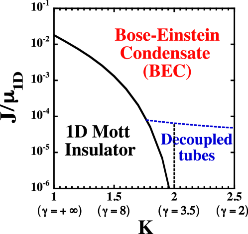
Figure 3: Zero-temperature phase diagram of a 2D array of coupled, finite, 1D interacting boson systems. The values on the vertical axis are defined up to a factor of order unity. $K$ is the Luttinger-liquid parameter (see section 2.2 for explanations). The corresponding values of Lieb-Liniger gas parameter $\gamma=Mg/\hbar^{2}\rho_{0}$ are also displayed. A longitudinal commensurate optical potential of amplitude $u_{0}$ ($u_{0}\approx 0.03\>\mu_{1D}$ for $K=1$ and $u_{0}\approx 0.02\>\mu$ for $K=2.5$) is assumed. The vertical dashed line describes the boundary between the (finite-sized) Tomonaga-Luttinger phase.

Let us consider a system of finite tubes in the BEC phase (i.e. the Mott potential is irrelevant or absent). In the limit of small $J$ ($J/\mu_{1D}\ll 1$) of interest here, the longitudinal fluctuations with wavenumber $q\neq 0$ can be integrated out as discussed in F. The resulting effective Hamiltonian is a quantum-phase model identical to the one used to describe a 2D array of Josephson junctions:

$$H_{\rm QP} = -E_{J}\sum_{\langle{\bf R},{\bf R^{\prime}}\rangle}\cos\left(\theta_{0{\bf R}}-\theta_{0{\bf R^{\prime}}}\right)$$ (88)

$$+\frac{E_{C}}{2}\sum_{\bf R}(N_{\bf R}-N_{0})^{2}-\mu\sum_{\bf R}N_{\bf R},$$

where $N_{\bf R}$ is the particle-number operator of tube at site $\bf R$, and $\theta_{0{\bf R}}$ the canonically conjugate phase operator: $[\theta_{0\bf R},N_{\bf R^{\prime}}]=i\delta_{{\bf R},{\bf R^{\prime}}}$. The renormalized hopping $E_{J}=E_{J}(N_{0})\simeq JN^{1-\frac{1}{2K}}_{0}$. The model (88) has been extensively studied in the literature (see e.g. Ref. [55] and references therein). It exhibits a quantum phase transition transition between a two-dimensional superfluid (2D SF) phase (a BEC at $T=0$) and a two-dimensional Mott insulator (2D MI) at a critical value of the ratio $E_{J}/E_{C}$. For commensurate filling (integer $N_{0}$) using Monte Carlo (MC) van Otterlo et al. [55] found $(E_{J}/E_{C})_{c}\simeq 0.15$. Using the forms for $E_{C}$ and $E_{J}$ derived above, and assuming that the tubes are described by the Lieb-Lininger model, the MC result reduces to $J_{c}/\mu_{1D}\simeq 0.3N^{-3/2}_{0}$ in the Tonks limit ($K=1$) and to $J_{c}/\mu_{1D}\simeq 0.15N^{-2}_{0}$ for weakly interacting bosons ($K\gg 1$) [20]. A similar result has been more recently obtained in Ref. [56] using the random phase approximation (RPA). Our result, however, includes critical fluctuations beyond the RPA as it relies on the numerically exact results from MC simulations. In figure 3 we show the complete zero-temperature phase diagram including the possibility of a phase where the tubes are effectively decoupled in a 2D MI phase (labeled Decoupled tubes in the diagram). Note that in the 2D MI, only the phase coherence between different tubes of the 2D lattice is lost. However, apart from the finite size-gap $\sim\hbar\pi v_{s}/L$, there is not gap for excitations in the longitudinal direction. This makes this phase different from the 1D MI described above, where there is a gap (depending very weakly on the size $L$) for longitudinal excitations. If the Mott potential is applied to the system in this phase, it will cross over to a 1D Mott insulator for a finite, but small value, of the dimensionless strength $g_{u}$. This crossover should take place for $K<2$ [2, 26, 17, 41] and is thus represented by a vertical dashed line in figure 3.

In the superfluid phase, the lattice will also exhibit a crossover as a function of temperature: If the condensation temperature $T_{c}$ found in section 3.1.2 is larger than the finite-size gap $\hbar v_{s}/L$, the gas should behave as a 3D BEC and cross over to a 2D SF for $T\sim\hbar v_{s}/L$. However, if $T_{c}\ll\hbar v_{s}/L$ the system should behave as a 2D quasi-condensate with no long range phase coherence (and therefore $\psi_{c}=0$) at finite temperature. Since $\hbar v_{s}/L\sim\hbar\omega_{0}$, $\omega_{0}$ being the longitudinal trapping frequency, and experimentally [7] $\omega_{0}\sim 0.1$ kHz whereas $T_{c}/\hbar\sim 10$ kHz, we expect to be in a regime where the BEC is always observed. The presence of harmonic confinement means that at least some of the tubes will have a filling deviating from commensurate filling. The critical value of $J/\mu_{1D}$ is reduced relative to the half-filled case, as shown in  figure 4.

Finally, let us estimate the typical value of the critical ratio $J_{c}/\mu_{1D}$. Using the above results and assuming that $\mu_{1D}\approx 0.1\>\hbar\omega_{\perp}$ [7] and $N_{0}=100$, we conclude that $J_{c}/\hbar\omega_{\perp}\simeq 10^{-4}$ for $K=1$ whereas $J_{c}/\hbar\omega_{c}\simeq 10^{-5}$ for $K\gg 1$. The deepest lattices used in the experiments of Refs. [7, 10] had $V_{\perp}=30\>E_{R}$, which corresponds to $J/\hbar\omega_{\perp}=5\times 10^{-5}$. This is of the same order of magnitude as $J_{c}/\hbar\omega_{\perp}$ for $K\gg 1$, although a larger number $N_{0}$ will further reduce this estimate, and therefore for this lattice the system may be well in the BEC phase (see figure 3). However, in the experiments [7, 10] no coherence was apparently observed between the tubes. The explanation for this contradiction is that the value of tunneling time $\hbar/J$ must be compared with the duration of the experiment $t_{\rm exp}$ and it turns out that for a lattice depth of $V_{0\perp}=30\>E_{R}$ this time is indeed longer than $t_{\rm exp}$. Therefore, over the duration of the experiment almost no tunneling process occurs and the build-up of intertube coherence can thus hardly take place.

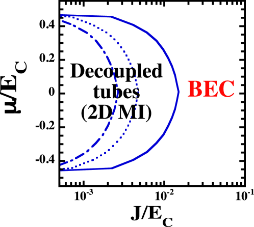
Figure 4: Phase diagram of a 2D array of finite 1D Bose gases as a function for the local chemical potential $\mu$ and the Josephson coupling $J$ for different values of the Luttinger parameter: $K=1$ ($\gamma\to+\infty$, continuous curve), $K=2$ ($\gamma=3.5$, dotted curve), $K=4$ ( $\gamma=0.71$, dash-dotted curve).

6 Comparison to experiments

In this section we discuss and summarize our results in connection with the recent experiments on anisotropic optical lattices [21, 7, 10, 22, 16, 13]. The complete phase diagram, taking into account the finiteness of the 1D gas tubes, is shown in figure 3. At zero temperature, we predict three phases: an anisotropic BEC, a 1D Mott insulator, and a phase where the gas tubes are decoupled (i.e. phase incoherent), namely a 2D Mott insulator.

However, as mentioned in section 2, the experimental systems are indeed harmonically confined. Unfortunately, so far it has proven very difficult to deal analytically and simultaneously with strong correlations and the harmonic trap. On the other hand, numerical methods can tackle this situation [30, 31, 32, 33, 34, 35]. In the harmonic trap, the cloud becomes inhomogeneous, and thus as demonstrated in a number of numerical simulations [33, 34, 35, 57, 58], for a wide range of system’s parameters, several phases can coexist in the same trap. These results have confirmed the experimental observations [12] as well as previous theoretical expectations based on mean-field calculations [24]. The numerical simulations have been mostly restricted to 1D systems [57, 33] and isotropic lattices [34], we expect most of their conclusions to also apply to the anisotropic optical lattices that interest us here. Thus, we also expect coexistence of the phases described above when the system is confined in a harmonic trap. Qualitatively, this indeed can be understood using the local density approximation, assuming that the trap potential gives rise to a local chemical potential which varies from point to point. Thus, from strong interactions we expect the formation of domains of the 1D Mott insulating phase near the center of the trap, whereas the superfluid phase should be located in the outer part of the cloud. If the transverse lattice is very deep (i.e. if $V_{0\perp}$ is large) there also can be regions where the number of boson per tube is small and the the phase coherence is lost because the charging energy $E_{C}$ becomes locally larger than $E_{J}$. Nevertheless, confirmation of this qualitative picture will require further experimental and numerical investigation, which we hope this work helps to motivate. The coexistence of different phases may be revealed by analyzing the visibility of the interference pattern observed in an expansion experiment [59, 58]. Let us finally mention that the existence of the trap can also lead to new and poorly understood phenomena such as suppression of quantum criticality [34].

Taking into account the above, we only aim at a qualitative description of some experimental observations. Thus, we have shown in 3.1.1 that the strong quantum fluctuations characteristic of 1D systems strongly deplete the condensate fraction in the BEC phase that forms for arbitrarily small intertube Josephson coupling. The condensate fraction can be as low as $\approx 10\,\%$ for typical experimental parameters ($V_{0\perp}=20\>E_{R}$). We have also argued that the experimentally measured coherence fractions may also include some of the non-condensate fraction, and therefore, provided heating effects of the sample in the measurement can be disregarded, the coherence fraction should be an upper bound to the BEC fraction. Quantum and thermal fluctuations are also responsible for the power-law behavior of the condensation temperature with $J/\mu_{1D}$. Estimates of the latter, when compared to the experimental estimates of the temperature of the lattice [7] and the finite-size excitation gap means that for $V_{0\perp}=20E_{R}$ the system should be in the BEC phase described in section 3 provided the Mott potential is sufficiently weak. In this phase, the system exhibits two kinds of low energy modes in the long wave-length limit: a gapless Goldstone mode, and a gapped longitudinal mode. Whereas the former corresponds to fluctuations of the phase of the order parameter, the latter is associated with fluctuations of its amplitude, namely the BEC density.

If the strength of the Mott potential is increased, the system (or at least part of it near the center of the trap) should undergo a deconfinement quantum phase transition (or crossover, given the finiteness of the sample) to a 1D Mott insulating phase. This phase is characterized by the existence of a gap in the excitation spectrum which is largely independent of the size of the tube. The hopping between the tubes is suppressed for temperatures (or energies) below this gap, and it is incoherent above it. For a deeper optical lattices, we predict that hopping between tubes can also be suppressed by the “charging energy” of the (finite-sized) tubes. We also notice that in some experiments the duration time of the experiment is also a limiting factor for the establishment of phase coherence even if hopping is not effectively suppressed by the charging energy.

Stöferle et al. [10] have studied an optical lattice system for several values of the depth of the transverse optical lattice potential (hence $J$). By analyzing the width of the momentum peak near ${\bf k}=0$ in the interference pattern after free expansion, they were able to deduce the energy absorption in response to a time-dependent modulation of the Mott potential. From this analysis, they could tell when the system behaves as a superfluid or as a Mott insulator. These experiments were analyzed recently [42, 60, 61, 62] and we will not repeat the conclusions of the analysis here. In the same series of experiments, they also studied the dependence of the width of the momentum peak near ${\bf k}=0$ in the ground state on the strength of the Mott potential, for several values of $V_{0\perp}$. For a BEC or a 1D superfluid, the inverse of the width is set by a geometrical factor and it is proportional to the size of the size of the cloud (or, in the 1D case, the thermal length $\hbar v_{s}/T$, whichever the shortest). For a Mott insulator, however, the inverse of the width is set by the correlation length $\xi_{c}\simeq\hbar v_{s}/\Delta_{c}$, where $\Delta_{c}$ is the Mott gap. Thus, an increase of the width as a function of the Mott potential reveal the opening of a gap in the spectrum of the system [33]. The experimental curves of the width as a function of the Mott potential present upturns around the points where the system should enter the Mott insulating phase in the thermodynamic limit. Our expectation, based on the phase diagram of figure 3, is that the deconfinement phase transition should take place for values of the Mott potential slightly larger than in the pure 1D case (represented by the vertical line at $K=2$ in figure 3). It is necessary to recall that, in the Bose-Hubbard model (cf. equation (6)) that describes the systems of Ref. [10], the Mott potential controls not only the dimensionless parameter $g_{u}$ that enters in the RG equations of section 4.1, but also the ratio of the interaction $U$ to the kinetic energy $J_{x}$, and therefore the Luttinger parameter $K$ as well. The latter decreases towards the Tonks limit ($K=1$) with increasing $U/J_{x}$. The theoretical expectation is in good qualitative agreement with the experimental observation.

The finite extent of trapped cloud (either longitudinally or transversally) limits the minimum momenta of the modes. Thus the energy of the lowest modes in the 3D SF phase can be directly estimated from our results by using the minimum available momentum in (40,41). For instance, for a finite 2D lattice containing $M_{y}\times M_{z}$ tubes (i.e. an atom cloud of size $L\times M_{y}a\times M_{z}a$) the lowest available momentum is $\sim\pi/(M_{i}a)$. Putting this value into (40,41) shows that the frequency of the lowest transverse modes decreases with decreasing $J$. This analysis neglects the possibility of phase coexistence described above, which calls for further investigation of these issues.

We have been not able to calculate the finite temperature excitation spectrum across the dimensional crossover, but it is interesting to speculate what happens to the Tomonaga-Luttinger liquid (TLL) spectrum, especially when the longitudinal momentum $q$ is near $2\pi\rho_{0}$. On general grounds, at temperatures large compared to the dimensional crossover scale $\sim T_{c}$, the system should exhibit essentially the 1D spectrum of a TLL, with its characteristic continuum of (particle-hole) excitations extending roughly between $q\approx 0$ and $q\approx 2\pi\rho_{0}$ [63]. As the temperature or the excitation frequency get below the crossover scale, the low-energy excitations around $2\pi\rho_{0}$ must disappear: being the BEC a 3D superfluid, by Landau’s criterion, there can be no low energy excitation that contributes to dissipation of superfluid motion. The gap about $q=2\pi\rho_{0}$ in the spectrum of the anisotropic BEC phase would be thus reminiscent of the roton gap in liquid Helium, which may be regarded as the remnant of the crystallization tendency at the momentum of where the roton minimum occurs [64]. In our case, because of the underlying 1D physics, the roton gap should have a continuum of excitations above it, which is the remnant of the 1D continuum of excitation in the TLL (see figure 5). This may account for the “relatively broad” energy absorption spectrum observed in the “1D to 3D crossover” regime in the experiment of Stöferle et al. [10, 42]

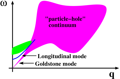
Figure 5: Schematic excitation spectrum of the BEC phase. Shaded lines and curves represent different types of excitations. The frequency of the excitation is $\omega$ and $q$ is momentum in the longitudinal direction (i.e. parallel to the tube axis). The continuum of particle and hole excitations stems from the spectrum a 1D system, as found by Lieb in Ref. [63]. At lower energies, however, the system develops the phase coherence characteristic of a BEC and therefore must obey Landau’s criterion of superfluidity. In particular, this means that the system must exhibit a gap at $q=2\pi\rho_{0}$, where $\rho_{0}$ is the linear density of the 1D system. In the long wave-length limit, we find the system exhibits two kinds of excitations: a gapless (Goldstone) mode, and a gapped longitudinal mode. There is also a continuum of excitations above the longitudinal mode (see discussion at the end of section 3.1.3).

7 Conclusions and discussion

In summary, through a variety of methods, we have arrived at the following picture For the case where the Mott potential is either absent, incommensurate, or generally, irrelevant in the RG , the existence of an arbitrarily weak intertube tunneling immediately turns the 1D arrays into a 3D BEC at zero temperature, albeit with anisotropic properties. At finite temperature, thermal fluctuations cause a phase transition at $T=T_{c}$ where the 3D coherence (and the BEC) is lost. Since $T_{c}\ll\mu_{1D}$ in the quasi-1D optical lattices studied here, for $T_{c}<T\ll\mu_{1D}$ the system behaves as a 2D array of phase-incoherent Tomonaga-Luttinger liquids. We have obtained explicit expressions for $T_{c}$, the condensate fraction at $T=0$, the excitation spectrum, and momentum distribution function, which could be compared to measurements in the experimental systems. In particular, the power-law behaviors of $J/\mu$ found for $T_{c}$ and condensate fraction are consequences of the strong fluctuations that dominate the properties of the uncoupled 1D systems. In the presence of a relevant (in the RG sense) Mott potential, a finite intertube tunneling ($J_{c}$) is required to overcome the localization tendencies of the interacting bosons. This process takes place in the form of a deconfinement quantum phase transition. Our main result in this case is the phase diagram shown in figure 3 as a function of $J/\mu_{1D}$ and the parameter $K$ characterizing the interactions in the tube. For the deconfinement transition, we also find a power-law dependence of $J_{c}$ on the strength of the Mott potential $u_{0}$, and a power-law dependence of the condensate fraction near the transition (indeed, these two results are strictly valid for $K=1/2$, which is outside the range of values for bosons with short-range interactions, but we speculate that these results are adiabatically connected to the physical (for bosons) regime of $K>1$ as we have found no evidence of any quantum phase transitions for $1/2\geq K\geq 1$ in our RG calculation.) Finally, for comparisons to experiments, we have looked into trap effects by studying tubes of finite length and described the transition where the system goes from a system of uncoupled 1D Luttinger liquids to the 3D superfluid as (renormalized) $J$ overcomes the “charging energy” of the finite length tube. As discussed in details in the previous section we can compare our predictions with the experiments of Stöferle et al. [10]. Some of our predictions, in particular the large reduction of the coherent fraction is in qualitative agreement with the experiment.

Clearly, further experimental and theoretical studies are needed to provide a more thorough and quantitative picture of the dimensional crossover and the deconfinement transition. From the theoretical point of view, taking into account the harmonic trap in a more quantitative way would be a step towards a more quantitative description of the experiments. From the experimental point of view, investigation of larger systems with more atoms per tube and more tubes, and in longer experiments that allow to probe smaller values of the Josephson coupling $J$, would permit a more complete exploration of the phase diagram of the quasi-1D lattices. Also, most of the current experiments in these lattices have been carried out using rather deep Mott potentials in order to reduce the ratio of kinetic to interaction energy (this is the regime where the Bose-Hubbard model of equation (6) is applicable). However, It would be very interesting to conduct experiments where the interaction energy between the atoms is tuned independently of the longitudinally applied (Mott) potential. Increasing the interaction strength in the absence of Mott potential was recently achieved by Kinoshita et al. [13] by confining the atoms in tighter 1D traps. Under these conditions, and for interaction strength $\gamma\approx 3.5$ [2, 41] in 1D, the application of the Mott potential of strength much smaller than the chemical potential $\mu_{1D}$ should suffice to cause localization of the bosons in the 1D Mott insulating phase. To the best of our knowledge, this “weak lattice” Mott insultator has not yet really been realized. In this phase quantum effects are stronger, and it would be then very interesting to drive the system across the deconfinement transition by changing $J$.

8 Acknowledgments

We thank T. Esslinger, A. Nersesyan, and M. Gunn for useful conversations and/or correspondence. MAC and AFH thank the hospitality of the University of Geneva where this work was started. AFH is funded by EPSRC (UK), MAC by Gipuzkoako Foru Aldundia and MEC (Spain) under Grant FIS2004-06490-C03-01. This work was supported in part by the Swiss National Science Foundation through MaNEP and division II.

Appendix A Mean-field theory (MFT) and gaussian fluctuations (RPA)

In this section we shall employ the functional integral to derive the mean-field Hamiltonian theory of section 3.1, and to go further by taking into account gaussian fluctuations about the mean-field state. The method is known as the random-phase approximation (RPA). Our treatment follows Ref. [65].

Let us consider the model defined by equation (11). Using the coherent-state path-integral, the partition function can be written as follows:

$$Z=\int\left[d\psi d\psi\right]\,e^{-S\left[\psi^{*},\psi\right]},$$ (89)

where the (euclidean) action,

$$S\left[\psi^{*},\psi\right]=\frac{1}{\hbar}\int^{\hbar\beta}_{0}d\tau\int^{L}_{0}dx\left[\sum_{\bf R}\psi^{*}_{\bf R}\left(\hbar\partial_{\tau}\psi_{\bf R}-\mu\psi_{\bf R}\right)+{\cal H}(\psi^{*}_{\bf R},\psi_{\bf R})\right],$$ (90)

${\cal H}(\psi^{*}_{\bf R},\psi_{\bf R})$ being the Hamiltonian density corresponding to equation (11). Since the Mott potential plays no role in the BEC phase (i.e. it is irrelevant in the RG sense), we drop it from the Hamiltonian ${\cal H}(\psi^{*}_{\bf R},\psi_{\bf R})$. However, the action $S\left[\psi^{*},\psi\right]$ still contains the non-trivial Josephson coupling between neighboring 1D systems.

$$S_{J}\left[\psi^{*}_{\bf R},\psi_{\bf R}\right] = -\frac{J}{\hbar}\sum_{\langle{\bf R},{\bf R}^{\prime}\rangle}\int^{\hbar\beta}_{0}d\tau\int^{L}_{0}dx\,\psi^{*}_{\bf R}(x,\tau)\psi_{\bf R^{\prime}}(x,\tau)$$ (91)

$$= -\sum_{{\bf R},{\bf R}^{\prime}}\int^{\hbar\beta}_{0}\frac{d\tau}{\hbar}\int^{L}_{0}dx\,\psi^{*}_{\bf R}(x,\tau)J_{{\bf R}-{\bf R}^{\prime}}\psi_{\bf R^{\prime}}(x,\tau).$$ (92)

In the above expression we have introduced the following notation:

$$J_{{\bf R}-{\bf R}^{\prime}}=J\>\sum_{\mathbf{t}}\delta_{{\bf R}^{\prime}-{\bf R}.\mathbf{t}},$$ (93)

where $\mathbf{t}$ runs over set of vectors that connect a lattice point to its nearest neighbors. We perform a Hubbard-Stratonovich (HS) decoupling of $S_{J}\left[\psi^{*},\psi\right]$:

$$e^{-S_{J}\left[\psi^{*},\psi\right]}={\cal N}\int\left[d\xi^{*}d\xi\right]\,e^{-\int^{\hbar\beta}_{0}\frac{d\tau}{\hbar}\int^{L}_{0}dx\,\left\{\sum_{{\bf R},{\bf R}^{\prime}}\ \xi^{*}_{\bf R}(x,\tau)J^{-1}_{{\bf R},{\bf R}^{\prime}}\xi_{{\bf R}^{\prime}}(x,\tau)+\sum_{\bf R}\left[\psi^{*}_{\bf R}(x,\tau)\xi_{\bf R}(x,\tau)+{\rm c.c.}\right]\right\}}$$ (94)

To make sense of $J^{-1}_{{\bf R}-{\bf R}^{\prime}}$ the Fourier transform of $J_{{\bf R},{\bf R}^{\prime}}$ is needed,

$$J({\bf Q})=J\sum_{\mathbf{t}}\>e^{i{\bf Q}\cdot\mathbf{t}}=2J\>\left[\cos Q_{y}a+\cos Q_{z}a\right].$$ (95)

The last result applies to a square lattice (in the OYZ plane) with lattice parameter $a$. Hence,

$$J^{-1}_{{\bf R}-{\bf R}^{\prime}}=\frac{1}{M_{0}}\sum_{{\bf Q}\in 1BZ}\>\frac{e^{i{\bf Q}\cdot\left({\bf R}-{\bf R}^{\prime}\right)}}{J({\bf Q})}.$$ (96)

Thus, after performing the HS decoupling, the action becomes:

$$S\left[\xi^{*},\xi,\psi^{*},\psi\right]=S_{B}\left[\psi^{*},\psi\right]+S_{J}\left[\xi^{*},\xi\right]+\int^{\hbar\beta}_{0}\frac{d\tau}{\hbar}\int^{L}_{0}dx\>\sum_{\bf R}\left[\xi^{*}_{\bf R}(x,\tau)\psi_{\bf R}(x,\tau)+{\rm c.c.}\right],$$ (97)

where

$$S_{B}\left[\psi^{*},\psi\right]=\int^{\hbar\beta}_{0}\frac{d\tau}{\hbar}\int^{L}_{0}dx\sum_{\bf R}\left[\psi^{*}_{\bf R}\left(\hbar\partial_{\tau}-\mu\right)\psi_{\bf R}+\frac{\hbar^{2}}{2M}\left|\partial_{x}\psi_{\bf R}\right|^{2}+\frac{g}{2}|\psi_{\bf R}|^{4}\right],$$ (98)

$$S_{J}\left[\xi^{*},\xi\right]=\int^{\hbar\beta}_{0}\frac{d\tau}{\hbar}\int^{L}_{0}dx\sum_{{\bf R},{\bf R}^{\prime}}\,\xi^{*}_{\bf R}(x,\tau)J^{-1}_{{\bf R}-{\bf R}^{\prime}}\xi_{\bf R^{\prime}}(x,\tau).$$ (99)

To perform the mean field approximation we formally integrate out the boson degrees of freedom described by $\psi_{\bf R}(x,\tau)$ and $\psi^{*}_{\bf R}(x,\tau)$, and obtain the effective action for the HS fields:

$$S_{GL}\left[\xi^{*},\xi\right] = S_{J}\left[\xi^{*},\xi\right]+S_{\psi}\left[\xi^{*},\xi\right],$$ (100)

$$\ S_{\psi}[\xi^{*},\xi] = -\ln\langle e^{-\int^{\hbar\beta}_{0}\frac{d\tau}{\hbar}\int^{L}_{0}dx\left[\xi^{*}_{\bf R}(x,\tau)\psi_{\bf R}(x,\tau)+\psi^{*}_{\bf R}(x,\tau)\xi_{\bf R}(x,\tau)\right]}\rangle_{\psi^{*},\psi}.$$ (101)

We have introduced the notation $S_{GL}$ for the effective action to indicate that it is indeed the GL functional.

To obtain the mean-field equations we perform a saddle-point expansion. The saddle-point is determined by the following equations:

$$\frac{\delta S_{GL}\left[\xi^{*},\xi\right]}{\delta\xi^{*}_{\bf R}(x,\tau)}=\frac{1}{\hbar}\sum_{{\bf R}^{\prime}}J^{-1}_{{\bf R}-{\bf R}^{\prime}}\xi_{{\bf R}^{\prime}c}(x,\tau)+\frac{\delta S_{\psi}[\xi^{*}_{c},\xi_{c}]}{\delta\xi_{\bf R}(x,\tau)}=0,$$ (102)

$$\frac{\delta S_{GL}\left[\xi^{*},\xi\right]}{\delta\xi({\bf R},x,\tau)}=\frac{1}{\hbar}\sum_{{\bf R}^{\prime}}\xi^{*}_{\bf R^{\prime}}(x,\tau)J^{-1}_{{\bf R}^{\prime}-{\bf R}}+\frac{\delta S_{\psi}[\xi^{*}_{c},\xi_{c}]}{\delta\xi^{*}_{\bf R}(x,\tau)}=0.$$ (103)

We look for uniform solutions to the above equations, i.e. $\xi_{\bf R}(x,\tau)=\xi_{c}$ and $\xi^{*}_{\bf R}(x,\tau)=\xi^{*}_{c}$. Furthermore, because of global gauge invariance, the particular choice for the phase of $\xi_{0}$ should not matter, that is, if $(\xi^{*}_{c},\xi_{c})$ is a saddle point then so is $(e^{-i\theta_{c}}\xi^{*}_{c},e^{i\theta_{c}}\xi_{c})$. Thus $S_{\psi}\left[\xi^{*}_{c},\xi_{c}\right]=S_{\psi}(|\xi_{c}|^{2})$. This implies that the above equations reduce to:

$$\frac{1}{M_{0}L\hbar\beta}S^{\prime}_{GL}(|\xi_{c}|^{2})=\frac{1}{\hbar}\sum_{\bf R}J^{-1}_{\bf R}+\frac{1}{M_{0}L\hbar\beta}S^{\prime}_{\psi}(|\xi_{c}|^{2})=0,$$ (104)

where the prime stands for the derivative with respect to $\rho_{\xi}=|\xi|^{2}$. Furthermore, using equation (101), equation (102) can also be written as:

$$\sum_{{\bf R}^{\prime}}J^{-1}_{{\bf R}-{\bf R}^{\prime}}\xi_{c}=-\langle\psi_{\bf R}(x,\tau)\rangle=-\psi_{c},$$ (105)

where it is understood that the expectation value of $\psi_{\bf R}(x,\tau)$ is taken by tracing out the boson degrees of freedom in the presence of the constant HS $(\xi^{*}_{c},\xi_{c})$, i.e. . using $S[\xi^{*}_{c},\xi_{c},\psi^{*},\psi]$ (cf. equation (97)). Therefore, (103) must be solved self-consistently for $(\xi^{*}_{c},\xi_{c})$: This is the self-consistency condition mentioned in section 3.1. Upon multiplying equation (105) by $J_{{\bf R}^{\prime\prime}-{\bf R}}$ from the left and summing over ${\bf R}$, we arrive at:

$$\xi_{c}({\bf R},x,\tau)=\xi_{c}=-z_{C}J\psi_{c},$$ (106)

where $z_{C}$ is the number of nearest neighbors ($z_{C}=4$ for a 2D square lattice). The above system of equations defines the mean field theory, which we have solved, in Hamiltonian form, in section 3.1.

We next take into account fluctuations by considering the gaussian corrections to the saddle point $(\xi^{*}_{c},\xi_{c})$. Let

$$\delta\xi_{\bf R}(x,\tau) = \xi_{\bf R}(x,\tau)-\xi_{c},$$ (107)

$$\delta\xi^{*}_{\bf R}(x,\tau) = \xi^{*}_{\bf R}(x,\tau)-\xi^{*}_{c}.$$ (108)

To proceed further we need to integrate out the boson degrees of freedom and obtain $S_{\psi}[\xi^{*},\xi]$ explicitly. Since we are interested in the properties at long wave-lengths and low frequencies and temperatures, we first apply bosonization and obtain:

$$S[\xi^{*},\xi,\theta]=\sum_{\bf R}S^{0}_{\bf R}[\theta]+S_{J}[\xi^{*},\xi]+\sqrt{{\cal A}_{B}\rho_{0}}\int^{\hbar\beta}_{0}\frac{d\tau}{\hbar}\int^{L}_{0}dx\>\sum_{\bf R}\left[\xi^{*}_{\bf R}(x,\tau)e^{i\theta_{\bf R}(x,\tau)}+{\rm c.c.}\right].\\$$ (109)

In the above expression,

$$S^{0}_{\bf R}[\theta]=\frac{K}{2\pi}\int^{\hbar\beta}_{0}d\tau\int^{L}_{0}dx\left[\frac{1}{v_{s}}\left(\partial_{\tau}\theta_{\bf R}(x,\tau)\right)^{2}+v_{s}\left(\partial_{x}\theta_{\bf R}(x,\tau)\right)^{2}\right].$$ (110)

In this (bosonized) form, integrating out the boson degrees of freedom amounts to tracing out the phase field $\theta_{\bf R}(x,\tau)$. This will carried out in what follows using the cumulant expansion:

$$\ln\Bigl{\langle}e^{-A\left[\xi^{*},\xi,\theta\right]}\Bigr{\rangle}_{sG}=-\langle A\left[\xi^{*},\xi,\theta\right]\rangle_{sG}+\frac{1}{2}\bigl{\langle}\big{(}A\left[\xi^{*},\xi,\theta\right]-\langle A\left[\xi^{*},\xi,\theta\right]\rangle_{sG}\big{)}^{2}\bigr{\rangle}_{\rm sG}+\cdots$$ (111)

where $\langle\ldots\rangle_{sG}$ denotes the trace over (smooth) configurations of $\theta_{\bf R}(x,\tau)$ using the weight $e^{-S[\xi^{*}_{c},\xi_{c},\theta]}$ (cf. equation ( 109), note that this action defines a collection of independent sine-Gordon models, which explains the notation). The RPA corresponds to keeping the terms of the above expansion up to quadratic order in $\delta\xi$ and $\delta\xi^{*}$. Thus, using that

$$A\left[\xi^{*},\xi,\theta\right]=\int^{\hbar\beta}_{0}\frac{d\tau}{\hbar}\int^{L}_{0}dx\sum_{\bf R}\left[\xi^{*}_{\bf R}(x,\tau)e^{i\theta_{\bf R}(x,\tau)}+e^{-i\theta_{\bf R}(x,\tau)}\xi_{\bf R}(x,\tau)\right],$$ (112)

we obtain:

$$S_{\psi}\left[\xi^{*},\xi\right] = \frac{1}{\hbar}\sqrt{\rho_{0}{\cal A}_{B}}\>\int^{\hbar\beta}_{0}d\tau\int^{L}_{0}dx\sum_{\bf R}\left[\delta\xi^{*}_{\bf R}(x,\tau)\,\langle e^{i\theta_{\bf R}(x,\tau)}\rangle+\langle e^{-i\theta_{\bf R}(x,\tau)}\rangle\,\delta\xi_{\bf R}(x,\tau)\right]$$ (113)

$$-\frac{\rho_{0}{\cal A}_{B}}{2\hbar^{2}}\int^{\hbar\beta}_{0}d\tau\>d\tau^{\prime}\int^{L}_{0}dx\>dx^{\prime}\>\sum_{{\bf R},{\bf R^{\prime}}}\>\Big{[}\langle\langle e^{-i\theta_{\bf R}(x,\tau)}e^{-i\theta_{\bf R^{\prime}}(x^{\prime},\tau^{\prime})}\rangle\rangle\>\delta\xi^{*}_{\bf R}(x,\tau)\>\delta\xi^{*}_{\bf R^{\prime}}(x^{\prime},\tau^{\prime})$$

$$+\langle\langle e^{-i\theta_{\bf R}(x,\tau)}e^{-i\theta_{\bf R^{\prime}}(x^{\prime},\tau^{\prime})}\rangle\rangle\>\delta\xi_{\bf R}(x,\tau)\>\delta\xi_{\bf R^{\prime}}(x^{\prime},\tau^{\prime})$$

$$+2\langle\langle e^{i\theta_{\bf R}(x,\tau)}e^{-i\theta_{\bf R^{\prime}}(x^{\prime},\tau^{\prime})}\rangle\rangle\>\delta\xi^{*}_{\bf R}(x,\tau)\>\delta\xi_{\bf R^{\prime}}(x^{\prime},\tau^{\prime})\Big{]}+\cdots$$

We have introduced the following notation:

$$\langle\langle F[\theta(x,\tau)G[\theta(x^{\prime},\tau^{\prime})]\rangle\rangle = \langle\left(F[\theta(x,\tau)]-\langle F[\theta(0,0)]\rangle_{sG}\right)$$ (114)

$$\times\left(G[\theta(x^{\prime},\tau^{\prime})]-\langle G[\theta(0,0)]\rangle_{sG}\right)\rangle_{\rm sG},$$

with

$$\langle F[\theta(x,\tau)]\rangle_{\rm sG}=\frac{\int\left[d\theta\right]\,F[\theta(x,\tau)]\,e^{-S_{\rm sG}[\theta,\xi^{*}_{c},\xi_{c}]}}{\int\left[d\theta\right]e^{-S_{\rm sG}[\theta,\xi^{*}_{c},\xi_{c}]}}$$ (115)

and

$$S_{sG}[\theta,\xi^{*}_{c},\xi_{c}] = \frac{K}{2\pi}\int^{\hbar\beta}_{0}d\tau\int^{L}_{0}dx\sum_{\bf R}\left[\frac{1}{v_{s}}\left(\partial_{\tau}\theta_{\bf R}(x,\tau)\right)^{2}+v_{s}\left(\partial_{x}\theta_{\bf R}(x,\tau)\right)^{2}\right]$$ (116)

$$+\sqrt{{\cal A}_{B}\rho_{0}}\>\int^{\hbar\beta}_{0}\frac{d\tau}{\hbar}\int^{L}_{0}dx\sum_{\bf R}\left[\xi^{*}_{c}\,e^{i\theta_{\bf R}(x,\tau)}+{\rm c.c.}\right].$$

Since in this action the different lattice sites are uncoupled, the correlation functions are diagonal in $\bf R$ and $\bf R^{\prime}$. Thus we can write the quadratic action that describes the (gaussian) fluctuations around the saddle point as follows:

$$S^{\rm RPA}_{GL}[\Xi^{{\dagger}},\Xi]=\frac{1}{2\hbar}\int^{\hbar\beta}_{0}d\tau\>d\tau^{\prime}\int dx\>dx^{\prime}\sum_{{\bf R},{\bf R}^{\prime}}\>\Big{[}\Xi^{{\dagger}}_{\bf R}(x,\tau){\bf J}^{-1}_{{\bf R}-{\bf R}^{\prime}}(x-x^{\prime},\tau-\tau^{\prime})\Xi_{\bf R^{\prime}}(x^{\prime},\tau^{\prime})$$

$$+\left(\Xi^{{\dagger}}_{\bf R}(x,\tau)+Q^{{\dagger}}_{\bf R}(x,\tau)\right){\bf G}_{{\bf R}-{\bf R}^{\prime}}(x-x^{\prime},\tau-\tau^{\prime})\left(\Xi_{\bf R^{\prime}}(x^{\prime},\tau^{\prime})+Q_{\bf R^{\prime}}(x^{\prime},\tau^{\prime})\right)\Big{]}$$ (117)

Note that the terms in $S^{\rm RPA}_{GL}$ linear in $\Xi$ and $\Xi^{{\dagger}}$ vanish because we expand around the saddle point. We have also dropped the constant term that is proportional to the mean field free energy. In the above expression the following spinors have been introduced:

$$\Xi_{\bf R}(x,\tau) = \left[\begin{array}[]{c}\delta\xi_{\bf R}(x,\tau)\\ \delta\xi^{*}_{\bf R}(x,\tau)\end{array}\right],Q_{\bf R}(x,\tau)=\left[\begin{array}[]{c}q_{\bf R}(x,\tau)\\ q^{*}_{\bf R}(x,\tau)\end{array}\right]$$ (122)

$$\Xi^{{\dagger}}_{\bf R}(x,\tau) = \left[\begin{array}[]{cc}\delta\xi^{*}_{\bf R}(x,\tau)&\delta\xi_{\bf R}(x,\tau)\end{array}\right],$$ (124)

$$Q^{{\dagger}}_{\bf R}(x,\tau) = \left[\begin{array}[]{cc}q^{*}_{\bf R}(x,\tau)&q_{\bf R}(x,\tau)\end{array}\right],$$ (126)

where we have introduced the sources $q^{*}_{\bf R}(x,\tau)$ and $q_{\bf R},x,\tau)$, which in the original action are coupled to $\psi_{\bf R}(x,\tau)-\psi_{c}$ and $\psi^{*}_{\bf R}(x,\tau)-\psi^{*}_{c}$, respectively. The matrices:

$${\bf J}^{-1}_{{\bf R}-{\bf R^{\prime}}}(1-2) = J^{-1}_{{\bf R}-{\bf R}^{\prime}}\delta(x-x^{\prime})\delta(\tau-\tau^{\prime})\>{\rm diag}\left[1,1\right],$$ (127)

$${\bf G}_{{\bf R}-{\bf R^{\prime}}}(1,2) = \left[\begin{array}[]{cc}g^{+-}_{1}(1,2)&e^{+2i\theta_{c}}g^{++}_{1}(1,2)\\ e^{-2i\theta_{c}}g^{--}_{1}(1,2)&g^{-+}_{1}(1,2)\end{array}\right],$$ (130)

with $1=({\bf R},x,\tau)$ and $2=({\bf R}^{\prime},x^{\prime},\tau^{\prime})$, and ($p,q=\pm$):

$$g^{pq}_{1}(1,2)=-\frac{{\cal A}_{B}\rho_{0}}{\hbar}\langle\langle e^{ip\theta_{\bf R}(x,\tau)}e^{iq\theta_{\bf R}(x^{\prime},\tau^{\prime})}\rangle\rangle_{\rm sG}\>\delta_{{\bf R}-{\bf R}^{\prime},\mathbf{0}}\,\,,$$ (131)

To perform the averages using $S_{sG}$ a gauge transformation is applied $\theta_{\bf R}(x,\tau)-\theta_{c}\to\theta_{\bf R}(x,\tau)$ so that $\xi_{c}=-z_{C}J\psi_{c}$ can be treated as a real number.

Let us now pause to consider the consequences of global gauge invariance on the correlation functions of (131). As we have found above, the GL functional is a function of $|\xi_{c}|^{2}$ only. Thus, if we expand $S_{\psi}(|\xi|^{2})$ around the saddle point solution:

$$S_{\psi}(|\xi|^{2})=S_{\psi}(|\xi_{c}|^{2})+\frac{\partial S_{\psi}}{\partial\xi}(|\xi_{c}|^{2})\delta\xi+\frac{\partial S_{\psi}}{\partial\xi}(|\xi_{c}|^{2})\delta\xi^{*}+\frac{1}{2!}\frac{\partial^{2}S_{\psi}}{\partial\xi^{2}}(|\xi_{c}|^{2})(\delta\xi)^{2}$$

$$+\frac{1}{2!}\frac{\partial^{2}S_{\psi}}{\partial\xi^{*2}}(|\xi_{c}|^{2})(\delta\xi^{*})^{2}+\frac{\partial S_{\psi}}{\partial\xi\partial\xi^{*}}(|\xi_{c}|^{2})|\delta\xi|^{2}+\cdots$$ (132)

where

$$\frac{\partial^{2}S_{\psi}}{\partial\xi^{2}}(|\xi_{c}|^{2})=\xi^{2}_{c}\>S^{\prime\prime}_{\psi}(|\xi_{c}|^{2}),$$ (133)

$$\frac{\partial^{2}S_{\psi}}{\partial\xi\partial\xi^{*}}(|\xi_{c}|^{2})=S^{\prime}_{\psi}(|\xi_{c}|)^{2}\>+|\xi_{c}|^{2}S^{\prime\prime}_{\psi}(|\xi_{c}|^{2}).$$ (134)

Using equation (104), $S^{\prime}_{\psi}(|\xi_{0}^{2}|)=-(M_{0}L\beta)\>\sum_{\bf R}J^{-1}_{\bf R}=-(M_{0}L\beta)\>\left[J({\bf Q}=0)\right]^{-1}$. Thus, by setting $\delta\xi^{*},\delta\xi={\rm const.}$ and taking $\beta\to\infty$ in equation (113), and comparing with equation (132), the following results can be obtained:

$$\tilde{g}_{1}(q=0,\omega=0)=g^{++/--}(q=0,\omega=0)=\frac{e^{2i\theta_{c}}}{M_{0}L\beta}\frac{\partial^{2}S_{\psi}}{\partial\xi^{2}}(|\xi_{c}|^{2})=\hbar\frac{\partial^{2}{\cal E}_{sG}}{\partial\xi^{2}},$$ (135)

$$g_{1}(q=0,\omega=0)=g^{+-/-+}(q=0,\omega=0)=\frac{1}{M_{0}L\beta}\frac{\partial^{2}S_{\psi}}{\partial\xi\partial\xi^{*}}(|\xi_{c}|^{2})=\hbar\frac{\partial^{2}{\cal E}_{sG}}{\partial\xi\partial\xi^{*}},$$ (136)

where we have used that $\lim_{\beta\to+\infty}S_{\psi}(|\xi_{c}|^{2})/(M_{0}L\hbar\beta)={\cal E}_{sG}(|\xi_{c}|^{2})$ is the energy density of the sine-Gordon model, equation (19). We shall use the above identities to calculate of the energy dispersion of the modes in the BEC phase. This phase exists below the critical temperature ($T_{c}$ to be determined below), and is characterized by having $\psi_{c}\propto\xi_{c}\neq 0$ so that global gauge symmetry is spontaneously broken. To compute the excitation spectrum in this phase, we diagonalize the matrix ${\bf J}^{-1}+{\bf G}$ (henceforth we drop the index ${\bf R}-{\bf R}^{\prime}$). ${\bf J}^{-1}$ is already diagonal, whereas the matrix ${\bf G}$ is rendered diagonal by:

$${\bf U}=\frac{1}{\sqrt{2}}\left[\begin{array}[]{cc}e^{i\theta_{c}}&e^{i\theta_{c}}\\ e^{-i\theta_{c}}&-e^{-i\theta_{c}}\end{array}\right].$$ (139)

Thus,

$${\bf C}(q,\omega_{n})={\bf U}^{{\dagger}}{\bf G}(k,\omega_{n}){\bf U}=\left[\begin{array}[]{cc}g_{1}(q,\omega_{n})+\tilde{g}_{1}(q,\omega_{n})&0\\ 0&g_{1}(q,\omega_{n})-\tilde{g}_{1}(q,\omega_{n})\end{array}\right],$$ (140)

where $\tilde{g}_{1}(q,\omega_{n})$ is the Fourier transform anomalous correlator $g^{++}_{1}(x,\tau)=g^{--}_{1}(x,\tau)$. In what follows we denote the eigenvalues of ${\bf G}(q,\omega_{n})$ as $c_{\pm}(q,\omega_{n})=g_{1}(q,\omega_{n})\pm\tilde{g}_{1}(q,\omega_{n})$. Next we express $S^{\rm RPA}_{GL}$ in terms of the eigenvectors of ${\bf G}(q,\omega)$ and to subsequently integrate out the transformed HS fields. In the following we use a matrix notation where the summations over ${\bf R},{\bf R^{\prime}}$ as well as over $q,\omega_{n}$ and multiplication by $\hbar^{-1}$ are implicitly understood. Hence,

$$S^{\rm RPA}_{GL}\left[\Xi^{{\dagger}},\Xi,Q^{{\dagger}},Q\right]=\frac{1}{2}\left[\Xi^{{\dagger}}\left({\bf J}^{-1}+{\bf G}\right)\Xi+Q^{{\dagger}}{\bf G}Q+Q^{{\dagger}}{\bf G}\Xi+\Xi^{{\dagger}}{\bf G}Q\right].$$ (141)

Let us make the replacement ${\bf G}={\bf U}{\bf C}{\bf U}^{{\dagger}}$, so that

$$S^{\rm RPA}_{GL}\left[X^{{\dagger}},X,P^{{\dagger}},P\right]=\frac{1}{2}\left[X^{{\dagger}}\left({\bf J}^{-1}+{\bf C}\right)X+P^{{\dagger}}{\bf C}P+P^{{\dagger}}{\bf C}X+X^{{\dagger}}{\bf C}P\right],$$ (142)

where $X={\bf U}^{{\dagger}}\Xi$ ($X^{{\dagger}}=\Xi^{{\dagger}}{\bf U}$), and $P={\bf U}^{{\dagger}}Q$ ($P^{{\dagger}}=Q^{{\dagger}}{\bf U}$). We shall obtain the generating functional in terms of these new sources. We can now integrate over the auxiliary fields $X^{{\dagger}},X$. Since they are related to $\Xi^{{\dagger}},\Xi$ by a global unitary transformation the measure of the functional integral is not affected. Thus we are free to shift $X\to X-\left({\bf J}^{-1}+{\bf C}\right)^{-1}{\bf C}P$ and $X^{{\dagger}}\to X^{{\dagger}}-P^{{\dagger}}{\bf C}\left({\bf J}^{-1}+{\bf C}\right)^{-1}$, which yields

$$Z\left[P^{{\dagger}},P\right]=\int\left[dX^{{\dagger}}dX\right]\,e^{-\frac{1}{2}X^{{\dagger}}{\bf C}X-\frac{1}{2}P^{{\dagger}}\left({\bf C}-{\bf C}\frac{1}{{\bf J}^{-1}+{\bf C}}{\bf C}\right)P}={\cal N^{\prime}}e^{-\frac{1}{2}P^{{\dagger}}\left({\bf C}-{\bf C}\frac{1}{{\bf J}^{-1}+{\bf C}}{\bf C}\right)P},$$ (143)

where $\cal N^{\prime}$ is an unimportant constant. Although we have been careful to treat the matrices in the last expression as non-commuting, all of them are diagonal and the last expression can be simplified to:

$$Z\left[P^{{\dagger}},P\right]=Z[0,0]\>\exp\left[-\frac{1}{2}P^{{\dagger}}\frac{\bf C}{\mathbf{1}+{\bf J\>C}}P\right]$$ (144)

Thus, the system has two modes, whose propagation is described by $\mathbf{\Delta}={\bf C}({\bf 1}+{\bf J\>C})^{-1}$. When expressed in Fourier components this propagator reads:

$$\mathbf{\Delta}({\bf Q},q,i\omega_{n})=\left[\begin{array}[]{cc}\Delta_{+}({\bf Q},q,\omega_{n})&0\\ 0&\Delta_{-}({\bf Q},q,\omega_{n})\end{array}\right],$$ (147)

$$\Delta_{\pm}({\bf Q},q,\omega)=\frac{c_{\pm}(q,\omega_{n})}{{\bf 1}+J({\bf Q})c_{\pm}(q,\omega_{n})}$$ (148)

The excitations are poles of the propagator:

$$1+J({\bf Q})c_{\pm}(q,i\omega_{n}\to\omega_{\pm}(q,{\bf Q}))1+J({\bf Q})c^{R}_{\pm}(q,\omega_{\pm}(q,{\bf Q}))=0.$$ (149)

Before we solve these equations in detail, let us first demonstrate the existence of the Goldstone mode, namely that there is a solution of (149) at $\omega=0$ for $|{\bf Q}|$ and $q\to 0$. To this end, we use (135,136), which are a consequence of gauge invariance, together with  (132,134), to arrive at $c_{-}(q=0,\omega=0)=g_{1}(q=0,\omega=0)-\tilde{g}_{1}(q=0,\omega=0)=S^{\prime}_{\psi}(|\xi_{c}|^{2})/(M_{0}L\beta)$. Moreover, by virtue of equation (104), $c_{-}(q=0,\omega=0)=S^{\prime}_{\psi}(|\xi_{0}|^{2})/(M_{0}L\beta)=-\sum_{\bf R}J^{-1}_{\bf R}=-[J({\bf Q}=0)]^{-1}=-1/(Jz_{C})$. This implies that $\omega=0$ is a solution of equation (149) for $|{\bf Q}|,q\to 0$, as anticipated, and identifies the eigenvalue labeled as ’$-$’ as the dispersion of the Goldstone mode. We shall use the condition that $c_{-}(q=0,\omega=0)=-[J({\bf Q}=0)]^{-1}$ in the calculation of the full dispersion of this mode below. But before we proceed into this calculation we need to know more about the correlation functions $c_{\pm}(k,\omega)$ for general $k,\omega$. Let us for a bit return to real space; we first notice that

$$c_{+}(x,\tau) = g_{1}(x,\tau)+\tilde{g}_{1}(x,\tau)=-\frac{2}{\hbar}\left[{\cal A}_{B}\rho_{0}\,\langle\cos\theta(x,\tau)\cos\theta(0,0)\rangle_{\rm sG}-\psi^{2}_{c}\right],$$ (150)

$$c_{-}(x,\tau) = g_{1}(x,\tau)-\tilde{g}_{1}(x,\tau)=-\frac{2}{\hbar}{\cal A}_{B}\rho_{0}\,\langle\sin\theta(x,\tau)\sin\theta(0,0)\rangle_{\rm sG}.$$ (151)

To make contact with the notation of Ref. [66], we introduce $\Phi=\theta/\beta$, $\beta^{2}=\pi/K$, ${\bf x}=(v_{s}\tau,x)$, and $\mu=\sqrt{{\cal A}_{B}\rho_{0}}\xi_{c}/\hbar v_{s}=\sqrt{{\cal A}_{B}\rho_{0}}Jz_{C}\psi_{c}/\hbar v_{s}$. The excitations of such a sine-Gordon model are the solitons and anti-solitons. Furthermore, $\beta^{2}<4\pi$ (i.e. $K>\frac{1}{4}$) the model also has breather excitations [40, 17], which are soliton-anti-soliton bound states, and whose zero-momentum energies (“mass” gaps) are [40, 17]:

$$\Delta_{n}=2\Delta_{s}\sin(\pi pn/2),$$ (152)

with $p=\beta^{2}/(8\pi-\beta^{2})$, $n=1,2,\ldots,[p^{-1}]-1$, and $\Delta_{s}\sim\mu^{\frac{1}{2-{1}/{4K}}}$ is energy gap of the soliton (see equation (20)). The operators $\sin\beta\Phi({\bf x})$ and $\cos\beta\Phi({\bf x})$ have zero conformal spin and therefore can only create breathers (if they exist) or pairs of solitons and anti-solitons. Furthermore, since under charge conjugation [40],

$${\cal C}^{-1}\Phi{\cal C}=-\Phi.$$ (153)

it follows that

$${\cal C}^{-1}(\cos\beta\Phi){\cal C} = +\cos\beta\Phi,$$ (154)

$${\cal C}^{-1}(\sin\beta\Phi){\cal C} = -\sin\beta\Phi.$$ (155)

Thus the cosine operator can only have poles corresponding to breather states that are even under conjugation, whereas the sine can only have poles for breathers that are odd under conjugation. Taking all these facts into account we can write the spectral function of the correlators of these two operators [40]:

$$\rho^{\sin}_{\rm sG}(q,\omega) = 2\pi Z\sum_{n\,{\rm odd}}w_{n}\>\delta(\omega^{2}-v^{2}_{s}q^{2}-\Delta^{2}_{n})+\rho^{\sin}_{\rm s\bar{s}}(q,\omega),$$ (156)

$$\rho^{\cos}_{\rm sG}(q,\omega) = 2\pi Z\sum_{n\,{\rm even}}w_{n}\>\delta(\omega^{2}-v^{2}_{s}q^{2}-\Delta^{2}_{n})+\rho^{\cos}_{\rm s\bar{s}}(q,\omega),$$ (157)

where $\rho^{\sin,\cos}_{s\bar{s}}(q,\omega)$ describes the continuum of soliton and anti-soliton excitations. We have also used that the solitons with even quantum number $n$ are even and those with odd $n$ are odd under $\cal C$ [40]. To make further progress, we assume that the behavior of the above correlation functions is dominated by the lowest energy pole (single-mode approximation, SMA), i.e. the lowest breather $\Delta_{1}=2\Delta_{s}\sin(p\pi/2)$. Hence, the retarded correlation function:

$$c^{R}_{-}(q,\omega)\simeq\frac{z_{-}}{(\omega+i\epsilon)^{2}-v_{s}^{2}q^{2}-(\Delta_{1}/\hbar)^{2}},$$ (158)

where $\epsilon\to 0^{+}$. Since $c_{-}(q=0,\omega=0)=-\left[J({\bf Q}=0)\right]^{-1}=-1/(Jz_{C})$, this fixes the residue $z_{-}=\Delta^{2}_{1}/(Jz_{C}\hbar^{2})$. Hence, the dispersion of the Goldstone mode can be obtained from equation (149) (we consider a square lattice below):

$$1+\frac{\Delta^{2}_{1}\sum_{j=y,z}\cos Q_{j}a}{\omega^{2}_{-}(q,{\bf Q})-v_{s}^{2}q^{2}-(\Delta^{2}_{1}/\hbar^{2})}=0,$$ (159)

so that $\omega^{2}_{-}(q,{\bf Q})=(v_{s}q)^{2}+\frac{1}{2}\Delta^{2}_{1}\sum_{j=y,z}\left(1-\cos Q_{j}a\right)/\hbar^{2}\simeq(v_{s}q)^{2}+(\Delta_{1}a/2\hbar)^{2}{\bf Q}^{2}$, the last expression being valid for $|{\bf Q}|\ll a^{-1}$. However, we emphasize that note that as $K\to+\infty$ (i.e. the bosons become weakly interacting) the number of breather poles proliferate and the SMA may break down. Going beyond the SMA requires some knowledge of the spectral weights $w_{n}$. Instead, we show the same form of the dispersion for the lowest-energy Goldstone mode can be also obtained from the self-consistent Harmonic approximation described in section 3.2.

Using similar methods we can obtain the energy dispersion of the longitudinal mode, which is the solution of the equation:

$$1+J({\bf Q})c^{R}_{+}(q,\omega_{+}(q,{\bf Q}))=0.$$ (160)

We again resort to the SMA, but taking into account that this time the pole is given by the lowest energy breather that is even under $\cal C$, i.e. $\Delta_{2}=2\Delta_{s}\sin(\pi p)$. We first fix the pole reside $z_{+}$ by studying the limiting behavior of $c(q,\omega)$ as $q,\omega\to 0$. This can be obtained from (132,134), along with (135,136), which imply:

$$c_{+}(q=0,\omega=0) = g_{1}(q=0,\omega=0)+\tilde{g}_{1}(q=0,\omega=0)$$ (161)

$$= \frac{1}{M_{0}L\beta}\left[S^{\prime}_{\psi}(|\xi_{c}|^{2})+2|\xi_{c}|^{2}S^{\prime\prime}_{\psi}(|\xi_{c}|^{2})\right]=\frac{\hbar}{2}\frac{d^{2}{\cal E}_{\rm sG}}{d\xi_{c}^{2}}$$ (162)

$$= \frac{\hbar}{2(Jz_{C})^{2}}\frac{d^{2}{\cal E}_{\rm sG}}{d\psi^{2}_{c}}=-\frac{\hbar}{z_{C}J}\left(\frac{1}{8K-1}\right),$$ (163)

where we have used gauge invariance to set $\theta_{c}=0$ so that $|\xi_{c}|=\xi_{c}$, together with

$$\frac{d{\cal E}_{\rm sG}(\psi_{c})}{d\psi^{2}_{c}}=-\frac{2z_{C}J}{8K-1},$$ (164)

which can be directly obtained from the expressions for ${\cal E}_{sG}$ and $\psi_{c}$ in section 3.1. Hence, assuming that (SMA):

$$c^{R}_{+}(q,\omega)\simeq\frac{z_{+}}{(\omega+i\epsilon)^{2}-v_{s}^{2}q^{2}-(\Delta_{2}/\hbar)^{2}},$$ (165)

we find that $z_{+}/(\Delta_{2}/\hbar)^{2}=(z_{C}J)^{-1}\left[1/(8K-1)\right]$. If, within the SMA, we solve equation (160), we arrive at:

$$\omega^{2}_{+}(q,{\bf Q})=\Delta^{2}_{+}+v^{2}_{s}q^{2}+\frac{\Delta^{2}_{2}}{\hbar^{2}}\left(\frac{a^{2}}{8K-1}\right)F({\bf Q}),$$ (166)

where $\Delta^{2}_{+}=\Delta^{2}_{2}\>(8K-2)/(8K-1)$ is the energy gap of the longitudinal mode at $(q,{\bf Q})=(0,\mathbf{0})$, and $F({\bf Q})=a^{-2}\sum_{\bf t}\left(1-e^{i{\bf Q}\cdot{\bf t}}\right)/2$.

At the transition temperature, $T=T_{c}$, the order parameter $\psi_{c}=\xi_{c}=0$ and the matrix ${\bf J}^{-1}_{{\bf R}-{\bf R^{\prime}}}+{\bf G}_{{\bf R}-{\bf R^{\prime}}}$ becomes singular. For $\xi_{c}=0$, the anomalous correlators $g^{++}_{1}=g^{--}_{1}=0$, and $g^{+-}_{1}=g^{-+}_{1}=g_{1}$, which leads to:

$$J^{-1}_{{\bf R}-{\bf R}^{\prime}}\delta(x-x^{\prime})\delta(\tau-\tau^{\prime})+g_{1}(x-x^{\prime},\tau-\tau^{\prime})=0.$$ (167)

Upon multiplying by $J_{{\bf R^{\prime\prime}}-{\bf R}}$, summing over $\bf R$, and integrating over $x$ and $\tau$, we obtain:

$$\sum_{\bf R}J_{{\bf R}-{\bf R}^{\prime}}\int^{\hbar\beta}_{0}d\tau\int^{L}_{0}dx\>g_{1}(x,\tau)=z_{C}J\,g^{R}_{1}(q=0,\omega=0;T_{c})=-1.$$ (168)

This is precisely the same condition for the BEC temperature derived in section 3.1.2. The expression for $g^{R}_{1}(q,\omega)$, which is needed to obtain $T_{c}$ explicitly is evaluated in the appendix that follows this one.

Finally, to make connection with the discussion of section 3.1.3, we explain that the identification of the mode labeled as ‘$-$’ with the Goldstone mode and the one labeled as ‘$+$’ as the longitudinal mode is indeed quite natural. If we perform a gauge transformation such that $\theta_{c}=0$, the matrix $\bf U$ of equation (139) produces the transformation:

$$\delta\xi^{(-)}_{{\bf R}}(x,\tau) = \frac{1}{\sqrt{2}}\left[\delta\xi_{\bf R}(x,\tau)-\delta\xi_{\bf R}(x,\tau)\right],$$ (169)

$$\delta\xi^{(+)}_{{\bf R}}(x,\tau) = \frac{1}{\sqrt{2}}\left[\delta\xi_{\bf R}(x,\tau)+\delta\xi_{\bf R}(x,\tau)\right].$$ (170)

Let us consider (small) fluctuations of the order parameter of the form considered in section 3.1.3: $\delta\xi(x,\tau)\propto\delta\Psi_{c}(x,{\bf R},\tau)=\Psi_{c}(x,{\bf R},\tau)-\psi_{c}=\left[\psi_{c}+\eta_{c}(x,{\bf R},\tau)\right]e^{i\theta_{c}}-\psi_{c}\simeq\eta_{c}(x,{\bf R},\tau)+i\theta_{c}(x,{\bf R},\tau)$, and $\delta^{*}_{\bf R}(x,\tau)$ the complex conjugate. Hence $\delta\xi^{(-)}_{\bf R}(x,\tau)\propto i\theta_{c}(x,{\bf R},\tau)$ and $\delta\xi^{(+)}_{\bf R}(x,\tau)\propto\eta_{c}(x,{\bf R},\tau)$. Thus we see that $\delta\xi^{(-)}_{\bf R}(x,\tau)$ is related to fluctuations of the phase of the BEC, whereas $\delta\xi^{(-)}_{\bf R}(x,\tau)$ is related to fluctuations of its amplitude.

Appendix B Finite-temperature phase susceptibility

In this appendix we compute the Fourier transform of the retarded phase-susceptibility of a 1D system of interacting bosons. This correlation function is to leading order the one-body boson Green’s function:

$$g_{1}(x,\tau,T)=-\frac{1}{\hbar}\langle{\cal T}\left[\Psi_{\bf R}(x,\tau)\Psi^{{\dagger}}_{\bf R}(0)\right]\rangle\simeq\frac{1}{\hbar}J\rho_{0}{\cal A}_{B}\langle e^{i\theta_{\bf R}(x,\tau)}e^{i\theta_{\bf R}(0,0)}\rangle.$$ (171)

In the above expression, we have replaced the boson field by its bosonized form to leading order:

$$\Psi_{\bf R}(x,\tau)\simeq\rho^{1/2}_{0}{\cal A}^{1/2}_{B}\>e^{i\theta_{\bf R}(x,\tau)}.$$ (172)

where ${\cal A}_{B}={\cal A}_{B}(K)$ is a non-universal prefactor. To compute this correlation function, the (gaussian) action (110) must be used. Either by direct computation using functional integrals [17], or by means of a conformal transformation of the correlation function at $T=0$ [37], one obtains the following result:

$$g_{1}(x,\tau,T)=-\frac{1}{\hbar}\rho_{0}{\cal A}_{B}(K)\>\left(\frac{(\pi T/\hbar v_{s}\rho_{0})^{2}}{\sin\left[\pi T(v_{s}\tau+ix)/\hbar v_{s}\right]\sin\left[\pi T(v_{s}\tau-ix)/\hbar v_{s}\right]}\right)^{\frac{1}{4K}}$$ (173)

In order to obtain the retarded version of this correlation function, we shall use the relationship (see e.g. [17]):

$$g^{R}_{1}(x,t,T)=-2\theta(t)\>{\rm Im}\>g^{F}_{1}(x,t,T).$$ (174)

where $g^{F}_{1}(x,t,T)$ is the time-ordered (à la Feynman) propagator. The latter can be obtained from (171) by analytical continuation: $\tau=it+\epsilon(t)$, where $\epsilon(t)={\rm sgn}(t)\epsilon$ ($\epsilon\to 0^{+}$). Hence,

$$g^{F}_{1}(x,t,T)=-\frac{1}{\hbar}\rho_{0}{\cal A}_{B}(K)\>\left(\frac{(\pi T/\hbar v_{s}\rho_{0})^{2}}{\sinh\left[\pi T(x+v_{s}t_{\epsilon}/\hbar v_{s}\right]\sinh\left[\pi T(x-v_{s}t_{\epsilon})/\hbar v_{s}\right]}\right)^{\frac{1}{4K}},$$ (175)

where $t_{\epsilon}=t-i\epsilon(t)$. We next exponentiate the above result and use that

$$R(x,t) = \sinh\left[\pi T(x+v_{s}t-iv_{s}\epsilon(t))/\hbar v_{s}\right]\sinh\left[\pi T(x-v_{s}t+iv_{s}\epsilon(t))/\hbar v_{s}\right]$$ (177)

$$= \sinh\left[\pi T(x+v_{s}t)/\hbar v_{s}\right]\sinh\left[\pi T(x-v_{s}t)/\hbar v_{s}\right]$$

$$+i\epsilon\>\left(\frac{\pi T}{\hbar}\right)\left|\sinh\left(\frac{2\pi Tt}{\hbar}\right)\right|+{\rm O}(\epsilon^{2}),$$

which follows upon expanding in powers of $\epsilon$, as well as the identity $\ln(a+i\epsilon)=\ln|a|+i\pi\theta(-a)$ (the branch cut of the logarithm is put on the negative real axis). Thus, the imaginary part of $g^{F}_{1}(x,t,T)$ does not vanish provided that ${\rm Re}\>R(x,t)<0$, that is, if $\sinh\left[\pi T(x+v_{s}t)/\hbar v_{s}\right]\sinh\left[\pi T(x-v_{s}t)/\hbar v_{s}\right]=-\sinh\left[\pi T\xi_{+}/\hbar v_{s}\right]\sinh\left[\pi T\xi_{-}/\hbar v_{s}\right]<0$, i.e. for $\xi_{+}\xi_{-}>0$ ($\xi_{\pm}=v_{s}t\pm x$). Therefore,

$${\rm Im}\>g^{F}_{1}(\xi_{+},\xi_{-},T)=-\rho_{0}{\cal A}_{B}(K)\left(\frac{\pi T}{\hbar v_{s}\rho_{0}}\right)^{\frac{1}{2K}}e^{-\frac{1}{4K}\ln{\rm Re}\>R(\xi_{+},\xi_{-})}\>{\rm Im}\>\exp\left[-\frac{i\pi}{4K}\theta(\xi_{-})\theta(\xi_{+})\right]$$

$$=D(K)\>\left(\frac{\pi T}{\hbar v_{s}\rho_{0}}\right)^{\frac{1}{2K}}\left|\frac{1}{\sinh\left[\pi T\xi_{+}/\hbar v_{s}\right]\sinh\left[\pi T\xi_{-}/\hbar v_{s}\right]}\right|^{1/4K}\>\theta(\xi_{-})\theta(\xi_{+}),$$ (178)

where $D(K)=\rho_{0}{\cal A}_{B}(K)\sin\left(\frac{\pi}{4K}\right)/\hbar$. Since we are interested in the Fourier transform of $g^{R}_{1}(x,t,T)$, it is convenient to express it in terms of the imaginary part of $g^{F}_{1}(x,t,T)$:

$$g^{R}_{1}(k,\omega,T) = -2\int^{+\infty}_{-\infty}dt\int^{+\infty}_{-\infty}dxe^{-ikx+i\omega t}\,g^{R}_{1}(x,t,T)$$ (179)

$$= -2\int^{+\infty}_{0}dt\int^{+\infty}_{-\infty}dx\,e^{-ikx+i\omega t}\>{\rm Im}\>g^{F}(x,t,T)$$ (180)

$$= -2\int^{+\infty}_{0}dt\int^{+v_{s}t}_{-v_{s}t}dx\,e^{-ikx+i\omega t}\>{\rm Im}\>g^{F}_{1}(x,t,T)$$ (181)

$$= -\frac{1}{v_{s}}\int^{+\infty}_{0}d\xi_{+}\int^{+\infty}_{0}d\xi_{-}\,\,e^{i(k_{+}\xi_{-}+k_{-}\xi_{+})/2}\,{\rm Im}\>g^{F}_{1}(\xi_{+},\xi_{-},T),$$ (182)

where we have used that $dt\>dx=d\xi_{+}d\xi_{-}/2v_{s}$ and have introduced $k_{\pm}=\omega/v_{s}\pm k$. In the third step we employed that ${\rm Im}\>g^{F}_{1}(x,t,T)$ is only non-zero for $-v_{s}t<x<v_{s}t$. Finally, we have expressed the integral in terms of “light-cone” coordinates $\xi_{\pm}$ to be able to benefit from the separability of ${\rm Im}\>g^{F}_{1}$ in terms of these coordinates. Hence,

$$g^{R}_{1}(k,\omega,T) = -\frac{D(K)}{v_{s}}\>\left(\frac{\pi T}{\hbar v_{s}\rho_{0}}\right)^{\frac{1}{2K}}f\left[\frac{\hbar v_{s}}{T}\left(\frac{\omega}{v_{s}}+q\right),K\right]f\left[\frac{\hbar v_{s}}{T}\left(\frac{\omega}{v_{s}}-q\right),K\right],$$ (183)

where (see e.g. [17]):

$$f\left(\frac{\hbar v_{s}q}{T},K\right)=\int^{+\infty}_{0}\>\frac{e^{ik\xi/2}d\xi}{\left|\sinh\left(\frac{\pi T\xi}{\hbar v_{s}}\right)\right|^{1/4K}}=2^{\frac{1}{4K}}\left(\frac{\hbar v_{s}}{2T}\right)B\left(\frac{1}{8K}-i\frac{\hbar v_{s}q}{4\pi T},1-\frac{1}{4K}\right),$$ (184)

$B(x,y)$ being the beta function, $B(x,y)=\Gamma(x)\Gamma(y)/\Gamma(x+y)$. In the calculation of the critical temperature we need the value of $g^{R}_{1}(k,\omega,T)$ for $q=0$ and $\omega=0$:

$$g^{R}_{1}(q=0,\omega=0;T)=-\pi^{2}\frac{D(K)}{v_{s}}\left(\frac{2\pi T}{\hbar v_{s}\rho_{0}}\right)^{1/2K-2}B^{2}\left(\frac{1}{8K},1-\frac{1}{4K}\right)$$ (185)

Appendix C Self-consistent Harmonic Approximation calculation

In this appendix, we fill in some of the details of the SCHA calculation. First, note that in equation (53), we can rewrite

$$\langle S-S_{\rm v}\rangle_{\rm v}=\frac{1}{2}\sum_{q,{\bf Q},\omega_{n}}G_{\rm v}(q,{\bf Q},\omega_{n})G^{-1}_{0}(q,\omega_{n})+\langle S_{\rm int}\rangle_{\rm v}-{\rm const.}.$$ (186)

Then, the variational approximation to the free energy becomes

$$F^{\prime}[G_{v}]=-\frac{1}{2}\sum_{q,{\bf Q},\omega_{n}}\ln G_{\rm v}(q,{\bf Q},\omega_{n})+\frac{1}{2}\sum_{q,{\bf Q},\omega_{n}}G_{\rm v}(q,{\bf Q},\omega_{n})G^{-1}_{0}(q,\omega_{n})+\langle S_{\rm int}\rangle_{\rm v},$$ (187)

where

$$\langle S_{\rm int}\rangle_{\rm v}=-{\cal A}_{B}\rho_{0}JL\beta\sum_{\langle{\bf RR^{\prime}}\rangle}{\rm Re}\;\exp\left[G_{\rm v}(0,{\bf R}-{\bf R^{\prime}},0)-G_{\rm v}(0,{\bf 0},0)\right],$$ (188)

and

$$G_{\rm v}(x,{\bf R}-{\bf R^{\prime}},\tau)=\frac{1}{M_{0}\hbar\beta L}\sum_{q,{\bf Q},\omega_{n}}e^{i{\bf Q}\cdot({\bf R}-{\bf R^{\prime}})+iqx-i\tau\omega_{n}}\;G_{\rm v}(q,{\bf Q},\omega_{n}),$$ (189)

In evaluating $\langle S_{\rm int}\rangle_{\rm v}$, we can take advantage of point group symmetry of the lattice in the perpendicular directions and replace $G_{\rm v}(0,{\bf R}-{\bf R^{\prime}},0)-G_{\rm v}(0,{\bf 0},0)$ inside the exponential by the more symmetric expression $\frac{1}{z_{c}}\sum_{{\bf R^{\prime}}={\bf R}+{\bf t}}G_{\rm v}(0,{\bf R}-{\bf R^{\prime}},0)-G_{\rm v}(0,{\bf 0},0)$, where ${\bf t}$ are the unit lattice vectors in the perpendicular directions. Then, the outer $\sum_{\langle{\bf RR^{\prime}}\rangle}$ just gives a factor of $z_{c}$. Taking the variational derivative of $F$, we get:

$$\frac{1}{G_{\rm v}(q,{\bf Q},\omega_{n})}=\frac{1}{G_{0}(q,\omega_{n})}-\frac{z_{C}{\cal A}_{B}(K)\rho_{0}}{2\hbar}J\,F({\bf Q})\,\,e^{\frac{2J}{z_{C}M_{0}L\hbar\beta}\sum_{q^{\prime},{\bf Q^{\prime}},\omega_{n}^{\prime}}F({\bf Q^{\prime}})\>G_{\rm v}(q^{\prime},{\bf Q^{\prime}},\omega_{n}^{\prime})},$$ (190)

with the free phonon propagator: $G^{-1}_{0}(q,\omega_{n})=\frac{K}{\pi v_{||}}\left[\omega^{2}_{n}+v^{2}_{||}q^{2}\right]\;\;$ ($v_{||}=v_{s}$), and $F({\bf Q})=\frac{a^{-2}}{2}\sum_{\bf t}\left(1-e^{{\bf Q}\cdot{\bf t}}\right)$. This single self-consistent equation for $G_{\rm v}(q,{\bf Q},\omega_{n})$ can be solved by rewriting it into two equations:

$$v^{2}_{\perp}=\frac{\pi z_{C}{\cal A}_{B}}{2K}(\rho_{0}a)\left(\frac{Ja}{\hbar}\right)v_{||}\>e^{\frac{2a^{2}}{z_{C}M_{0}L\hbar\beta}\sum_{q,{\bf Q},\omega_{n}}F({\bf Q})\>G_{\rm v}(q,{\bf Q},\omega_{n})},$$ (191)

$$G^{-1}_{\rm v}(q,{\bf Q},\omega_{n})=\frac{K}{\pi v_{||}}\left[\omega^{2}_{n}+(v_{||}q)^{2}+v^{2}_{\perp}\,F({\bf Q})\right].$$ (192)

Substituting equation (192) into (191), we get the equation for the variational parameter, the perpendicular phonon velocity $v_{\perp}$:

$$\ln\frac{v^{2}_{\perp}}{\frac{\pi z_{C}{\cal A}_{B}}{2K}(\rho_{0}a)\left(\frac{Ja}{\hbar}\right)v_{||}}=\frac{2a^{2}}{z_{C}M_{0}L\hbar\beta}\sum_{q,{\bf Q},\omega_{n}}F({\bf Q})\frac{\pi v_{||}/K}{\omega_{n}^{2}+v_{||}^{2}q^{2}+v_{\perp}^{2}F({\bf Q})}.$$ (193)

The Matsubara sum can be done to give:

$$\ln\frac{v^{2}_{\perp}}{\frac{\pi z_{C}{\cal A}_{B}}{2K}(\rho_{0}a)\left(\frac{Ja}{\hbar}\right)v_{||}}=\frac{\pi v_{||}}{K}I(T,v_{\perp})$$ (194)

with

$$I(T,v_{\perp})=\frac{2a^{2}}{z_{C}M_{0}L}\sum_{q,{\bf Q}}\frac{F({\bf Q})}{\left[v_{||}^{2}q^{2}+v_{\perp}^{2}F({\bf Q})\right]^{1/2}}\coth\frac{\left[v_{||}^{2}q^{2}+v_{\perp}^{2}F({\bf Q})\right]^{1/2}}{2T}.$$ (195)

We first study the variational equation (194) at zero temperature. At $T=0$, $\coth(x/2T)\rightarrow\rm{sign}(x)$. To perform the summations over momentum, we take the continuum approximation for both the parallel ($q$) and perpendicular (${\bf Q}$) momenta, with a cut-off for the parallel momentum to be $\Lambda=\mu_{1D}/v_{||}$ ($\mu_{1D}$ is the 1D chemical potential of an isolated tube). Thus, with $\frac{1}{M_{0}}\sum_{\bf Q}\longrightarrow a^{2}\int_{-\pi/a}^{\pi/a}\frac{dQ_{y}dQ_{z}}{(2\pi)^{2}}$, and $\frac{1}{L}\sum_{q}\longrightarrow\int_{-\Lambda}^{\Lambda}\frac{dq}{2\pi}$, we get:

$$I(0,v^{0}_{\perp})\approx\frac{1}{\pi v_{||}}\left[\ln\left(\frac{2\mu_{1D}}{v^{0}_{\perp}/a}\right)-\frac{B}{2}\right]$$ (196)

where $v_{\perp}^{0}=v_{\perp}(T=0)$ and

$$B=\frac{a^{2}}{2}\int_{-\pi}^{\pi}\frac{dQ_{x}dQ_{y}}{(2\pi)^{2}}\;F({\bf Q})\;\ln a^{2}F({\bf Q})\approx 0.836477.$$ (197)

Putting equations (196) and (194) together then gives equation (59) of Section 3.2. We have assumed here $v^{0}_{\perp}/a\ll\mu$. Otherwise, our starting point using the Haldane harmonic fluid construction is not valid in principle.

When $K\rightarrow\infty$ (towards the non-interacting Bose gas limit), ${\cal A}_{B}(K)\approx 1$, and using the Lieb and Liniger solution [1] we can show that $\mu_{1D}\approx v_{||}\rho_{0}\pi/K$. Thus, asymptotically for large $K$, we get:

$$\frac{v^{0}_{\perp}}{a\mu_{1D}}\simeq\frac{v^{0}_{\perp}}{v_{||}}\frac{K}{\rho_{0}a\pi}\longrightarrow\sqrt{\frac{z_{C}J}{\mu_{1D}}}.$$ (198)

Thus, $v_{\perp}^{0}/a<\mu_{1D}$ if and only if $z_{c}J<\mu_{1D}$. But since for the nearly free Bose gas, $\mu\propto 1/K^{2}$ is small, this demands a very hopping amplitude $J$.

In equation (59), there is a singularity as $K\rightarrow 1/4$, which is a signature that for $K<1/4$ the Josephson coupling becomes irrelevant in the RG sense. As this regime is beyond the reach for bosons with a Dirac-delta interaction, we will not consider it any further.

We now look at the variational equation (194) at finite temperature. First, defining $v_{\perp}(T_{c})=v_{\perp}^{c}$, we rewrite (194) as:

$$\left(\frac{v_{\perp}^{0}}{v_{\perp}^{c}}\right)^{1-1/4K}=\exp\frac{\pi v_{||}}{K}\left[I(T_{c},v_{\perp}^{c})-I(0,v_{\perp}^{c})\right].$$ (199)

Following Donohue[65], we approximate crudely $\coth(x)\approx 1/x$ for $|x|\leq 1$, and $\coth(x)\approx 1$ otherwise. Next, we develop a series expansion in $v_{\perp}^{c}/aT_{c}<1$ for the integrand in $I(T_{c},v_{\perp}^{c})-I(0,v_{\perp}^{c})$. It will turn out that at the transition $T=T_{c}$, $v_{\perp}^{c}$ is actually finite (i.e. first order transition) but less than $v_{\perp}^{0}$, and the expansion can be justified a posteriori, at least for $K$ not too close to 1. With the help of Mathematica to perform the expansion and to evaluate the resulting integrals, we find:

$$v_{||}\left(I(T_{c},v_{\perp}^{c})-I(0,v_{\perp}^{c})\right)\approx c_{-1}\frac{aT_{c}}{v_{\perp}^{c}}+c_{0}-\frac{1}{\pi}\ln\frac{z_{C}aT_{c}}{v_{\perp}^{c}}+\sum_{n=1}c_{2n}\left(\frac{v_{\perp}^{c}}{T_{c}a}\right)^{2n},$$ (200)

where $c_{-1}\approx 0.677473$, $c_{0}\approx 0.133129-1/\pi$, $c_{2}=5/96\pi$, $c_{4}=21/2560\pi$, $c_{6}=845/344604\pi$, $c_{8}=9415/9437184\pi$, $c_{10}=112203/230686720\pi$, $c_{12}=233695/872415232\pi$. We can show that the series converges quite rapidly for $v_{\perp}^{c}/aT_{c}<1$, but because this expression appears in an exponential, we need quite a few terms to get accurate trends, especially when $K$ gets close to $1$. Introducing this expansion into (199),

$$\frac{v_{\perp}^{c}}{v_{\perp}^{0}}=\left(\frac{z_{C}aT_{c}}{v_{\perp}^{0}}\right)^{1/4K}e^{-\frac{\pi}{4K}\left[c_{-1}\frac{aT_{c}}{v_{\perp}^{c}}+c_{0}+\sum_{n=1}c_{2n}\left(\frac{v_{\perp}^{c}}{aT_{c}}\right)^{2n}\right]}.$$ (201)

This equation is solved graphically for $(T_{c},v_{\perp}^{c}$) (the right hand side of (201) is an s-shaped curve that intersects the straight line of the lef hand side of (201) at 0, 1, or 2 points, as a function of $T_{c}$, and $v_{\perp}^{c}$; $T_{c}$ is, by definition, when the intersection is at one point only. We use Mathematica’s routine FindRoot to bracket this point to the desired accuracy.)

We thus find the following asymptotic results for $K\rightarrow\infty$:

$$\frac{aT_{c}}{v_{\perp}^{0}} \approx 0.610+0.698K,$$ (202)

$$\frac{v_{\perp}^{c}}{v_{\perp}^{0}} \approx 0.376+0.274/K.$$ (203)

Both asymptotes appear to hold good when $K\geq 4$. Dividing these equations, we get that $aT_{c}/v_{\perp}^{c}\approx 1.86K+0.270+\cdots$, thus justifying our expansion in $v_{\perp}^{c}/aT_{c}$, at least for $K\geq 4$. Combining with the asymptotic results for $\gamma_{0}$ as $K\rightarrow\infty$, we get the results quoted in section 3.2.

Appendix D Derivation of RG equations

In this appendix we show how to compute the RG flow to second order in the Josephson and Mott potential couplings. To this purpose, it is convenient to introduce the chiral fields $\phi_{{\bf R}+}(x)$ and $\phi_{{\bf R}-}(x)$, which are implicitly defined as follows:

$$\phi_{\bf R}(x) = \frac{\sqrt{K}}{2}\left[\phi_{{\bf R}+}(x)+\phi_{{\bf R}-}(x)\right],$$ (204)

$$\theta_{\bf R}(x) = \frac{1}{2\sqrt{K}}\left[\phi_{{\bf R}+}(x)-\phi_{{\bf R}-}(x)\right].$$ (205)

The effective Hamiltonian, equation (11), thus takes the form:

$$H_{\rm eff} = \frac{\hbar v_{s}}{4\pi}\sum_{\bf R}\int dx\left[\left(\partial_{x}\phi_{{\bf R}+}(x)\right)^{2}+\left(\partial_{x}\phi_{{\bf R}-}(x)\right)^{2}\right]$$ (206)

$$+\tilde{g}_{u}\sum_{\bf R}\int dx\>\cos\sqrt{K}\left(\phi_{{\bf R}+}(x)+\phi_{{\bf R}-}(x)\right)+\tilde{g}_{F}\>\sum_{\langle{\bf R},{\bf R}^{\prime}\rangle}\int dx\,\partial_{x}\phi_{{\bf R}+}(x)\partial_{x}\phi_{{\bf R}^{\prime}-}(x)$$

$$+\tilde{g}_{J}\sum_{\langle{\bf R},{\bf R^{\prime}}\rangle}\int dx\>\cos\left(\frac{\phi_{{\bf R}+}(x)-\phi_{{\bf R^{\prime}}+}(x)}{2\sqrt{K}}-\frac{\phi_{{\bf R}-}(x)-\phi_{{\bf R^{\prime}}-}(x)}{2\sqrt{K}}\right).$$

We have added here a term proportional to $\tilde{g}_{F}$, which is not present initially, but which is generated at second order in $\tilde{g}_{J}$ after integrating out short-distance degrees of freedom (see below). It represents a density interaction between nearest neighbor 1D systems.

We next introduce the chiral vertex operators $V^{+}_{\beta}({\bf R},\bar{z})=\,\,:e^{i\beta\phi_{{\bf R}+}(\bar{z})}:$ and $V^{-}_{\beta}({\bf R},z)=\,:e^{i\beta\phi_{{\bf R}-}(z)}:$, and define $z=v_{s}\tau+ix$ and $\bar{z}=v_{s}\tau-ix$, and $d^{2}z=v_{s}d\tau dx=dzd\bar{z}/2i$. To explicitly display the scaling dimensions of the various operators in $H_{\rm eff}$, we introduce the dimensionless couplings:

$$g_{u}=\pi a^{2}_{0}\tilde{g}_{u}/v_{s},\quad g_{J}=\pi a^{2}_{0}\tilde{g}_{J}/v_{s}\quad g_{F}=\pi\tilde{g}_{F}/v_{s},\quad g_{K}=\pi\tilde{g}_{K}/v_{s}.$$ (207)

Thus, the interactions are described by

$$S_{\rm int} = g_{K}\sum_{\bf R}\int\frac{d^{2}z}{2\pi}\,\bar{\partial}\phi_{{\bf R}+}(\bar{z})\partial\phi_{{\bf R}-}(z)+g_{F}\sum_{\langle{\bf R},{\bf R^{\prime}}\rangle}\int\frac{d^{2}z}{2\pi}\,\bar{\partial}\phi_{{\bf R}+}(\bar{z})\partial\phi_{{\bf R}^{\prime}-}(z)$$ (208)

$$+\frac{g_{u}}{a^{2-K}_{0}}\sum_{\bf R}\int\frac{d^{2}z}{2\pi}\,\left[V_{\sqrt{K}}^{+}({\bf R},\bar{z})V_{\sqrt{K}}^{-}({\bf R},z)+\left(\sqrt{K}\to-\sqrt{K}\right)\right]$$

$$+\frac{g_{J}}{a^{2-1/2K}_{0}}\sum_{\langle{\bf R},{\bf R^{\prime}}\rangle}\int\frac{d^{2}z}{2\pi}\>\Big{[}V^{+}_{\frac{1}{2\sqrt{K}}}({\bf R},\bar{z})V^{+}_{-\frac{1}{2\sqrt{K}}}({\bf R^{\prime}},\bar{z})V^{-}_{-\frac{1}{2\sqrt{K}}}({\bf R},z)V^{-}_{\frac{1}{2\sqrt{K}}}({\bf R^{\prime}},z)$$

$$+\left(\sqrt{K}\to-\sqrt{K}\right)\Big{]}$$

The RG is performed in real space on the perturbative expansion of the partition function $Z(a_{0})=Z_{0}\langle{\cal T}\exp\left[-S_{\rm int}\right]\rangle$. We first consider an infinitesimal change of the short distance cut-off $a_{0}\rightarrow a^{\prime}_{0}=(1+\delta\ell)a_{0}$, where $0<\delta\ell\ll 1$. Subsequently, we integrate out short-distance degrees of freedom in the range $a_{0}<|z|<a_{0}(1+\delta\ell)a_{0}$. Following Ref. [67], we use operator-product expansions (OPE) to evaluate expectation values of products of operators at two nearby points in space and time. For $z\to w$ (respectively, $\bar{z}\to\bar{w}$):

$$\partial\phi_{{\bf R}-}(z)\partial\phi_{{\bf R}-}(w)=-\frac{1}{(z-w)^{2}}+:\left[\partial\phi_{{\bf R}-}\left(\frac{z+w}{2}\right)\right]^{2}:\,+\cdots$$ (209)

$$\bar{\partial}\phi_{{\bf R}+}(\bar{z})\bar{\partial}\phi_{{\bf R}+}(\bar{w})=-\frac{1}{(\bar{z}-\bar{w})^{2}}+:\left[\bar{\partial}\phi_{{\bf R}+}\left(\frac{\bar{z}+\bar{w}}{2}\right)\right]^{2}:\,+\cdots$$ (210)

$$V^{+}_{\beta}({\bf R},\bar{z})V^{+}_{-\beta}({\bf R},\bar{w})=\frac{1}{(\bar{z}-\bar{w})^{\beta^{2}}}\left[1+i\beta(\bar{z}-\bar{z})\bar{\partial}\phi_{{\bf R}+}\left(\frac{\bar{z}+\bar{w}}{2}\right)+\cdots\right],$$ (211)

$$V^{-}_{\beta}({\bf R},z)V^{-}_{-\beta}({\bf R},w)=\frac{1}{(z-w)^{\beta^{2}}}\left[1+i\beta(z-w)\partial\phi_{{\bf R}-}\left(\frac{z+w}{2}\right)+\cdots\right].$$ (212)

$$\partial\phi_{{\bf R}-}(z)V^{-}_{\beta}({\bf R},w)=\frac{-i\beta}{z-w}V^{-}_{\beta}({\bf R},\frac{z+w}{2})+\cdots$$ (213)

$$\bar{\partial}\phi_{{\bf R}+}(\bar{z})V^{+}_{\beta}({\bf R},\bar{w})=\frac{-i\beta}{\bar{z}-\bar{w}}V^{+}_{\beta}({\bf R},\frac{\bar{z}+\bar{w}}{2})+\cdots$$ (214)

Therefore, we begin with by considering the perturbative expansion of the partition function at the new scale $a^{\prime}_{0}=(1+\delta\ell)a_{0}$,

$$Z((1+\delta\ell)a_{0},\left\{g_{i}(\ell+\delta\ell)\right\}) = 1+Z^{(1)}((1+\delta\ell)a_{0},\left\{g_{i}(\ell+\delta\ell)\right\})$$ (215)

$$+Z^{(2)}((1+\delta\ell)a_{0},\left\{g_{i}(\ell+\delta\ell)\right\})+\cdots,$$

where

$$Z^{(1)}((1+\delta\ell)a_{0},\left\{g_{i}(\ell+\delta\ell)\right\}) = -\langle S_{\rm int}\rangle,$$ (216)

$$Z^{(2)}((1+\delta\ell)a_{0},\left\{g_{i}(\ell+\delta\ell)\right\}) = \frac{1}{2!}\langle S^{2}_{\rm int}\rangle$$ (217)

The partition function must be left invariant by the RG transformation, i.e. $Z((1+\delta\ell)a_{0},\left\{g_{i}(\ell+\delta\ell)\right\})=Z(a_{0},\left\{g_{i}(\ell)\right\})$, provided that the couplings $\left\{g_{i}\right\}$ are properly transformed after integrating out the short-distance degrees of freedom in range defined by $a_{0}<|z-w|<(1+\delta\ell)a_{0}$.

At the lowest order (tree level), the couplings change only because of the explicit factors of $a_{0}$ (i.e. the scaling dimensions of the perturbing operators) in (208). Thus, the only couplings that change are:

$$g_{u}(\ell)=g_{u}(\ell+\delta\ell)(1+\delta\ell)^{-(2-K)}\\ \simeq g_{u}(\ell+\delta\ell)\left(1-(2-K(\ell)\delta\ell)\right),$$ (218)

and

$$g_{J}(\ell)=g_{J}(\ell+\delta\ell)(1+\delta\ell)^{-(2-1/2K)}\simeq g_{J}(\ell+\delta\ell)\left[1-\left(2-\frac{1}{2K(\ell)}\right)\delta\ell\right].$$ (219)

At second order, there are ten terms in the expansion of $Z^{(2)}[(1+\delta\ell)a_{0},\{g_{i}(\ell+\delta\ell)\}]$. As the manipulations are standard but rather long, we will just look at two of them in detail to illustrate the procedure. To see what kind of terms are generated from the product of two operators, we shall use “center-of-mass” coordinates: $u=z-w$ (respectively, $\bar{u}=\bar{z}-\bar{w}$) and $v=(z+w)/2$ (respectively, $\bar{v}=(\bar{z}+\bar{w})/2$), and we split the integrals of the operator products appearing at second order as follows:

$$\int\frac{d^{2}v}{2\pi}\int\limits_{(1+\delta\ell)a_{0}<|u|}\frac{d^{2}u}{2\pi}\,O_{1}(v+\frac{u}{2},\bar{v}+\frac{\bar{u}}{2})O_{2}(v-\frac{u}{2},\bar{v}-\frac{\bar{u}}{2})$$

$$=\int\frac{d^{2}v}{2\pi}\Bigg{[}\int\limits_{a_{0}<|u|}\frac{d^{2}u}{2\pi}-\int\limits_{a_{0}<|u|<(1+\delta\ell)a_{0}}\frac{d^{2}u}{2\pi}\Bigg{]}\,O_{1}(v+\frac{u}{2},\bar{v}+\frac{\bar{u}}{2})O_{2}(v-\frac{u}{2},\bar{v}-\frac{\bar{u}}{2})$$ (220)

The terms generated at second order by the RG transformation stem form the second integral, where the relative coordinate is restricted to the infinitesimal range $a_{0}<|u|<a_{0}(1+\delta\ell)$. To $O(g_{F}g_{J})$, there are two possible operator pairings because the hopping term couples operators from neighboring chains:

$$O(g_{F}g_{u}) = -\frac{1}{2!}\frac{g_{F}(\ell)g_{J}(\ell)}{a_{0}^{2-1/2K}}\sum_{\langle{\bf R},{\bf R}^{\prime}\rangle,\langle{\bf T},{\bf T}^{\prime}\rangle}\int\frac{d^{2}v}{2\pi}\int\limits_{a_{0}<|u|<(1+\delta\ell)a_{0}}\frac{d^{2}u}{2\pi}\Bigg{\{}\Bigl{\langle}\bar{\partial}\phi_{{\bf R}+}(\bar{v}+\frac{\bar{u}}{2})\partial\phi_{{\bf R^{\prime}}-}(v+\frac{u}{2})$$ (221)

$$\times\Big{[}V^{+}_{\frac{1}{2\sqrt{K}}}({\bf T},\bar{v}-\frac{\bar{u}}{2})V^{+}_{-\frac{1}{2\sqrt{K}}}({\bf T}^{\prime},\bar{v}-\frac{\bar{u}}{2})V^{-}_{-\frac{1}{2\sqrt{K}}}({\bf T},v-\frac{u}{2})V^{-}_{\frac{1}{2\sqrt{K}}}({\bf T}^{\prime},v-\frac{u}{2})$$

$$+\left(\sqrt{K}\to-\sqrt{K}\right)\Big{]}\Bigr{\rangle}\Bigg{\}}$$

Focusing on the terms where ${\bf R}={\bf T}$ and ${\bf R}^{\prime}={\bf T}^{\prime}$, or ${\bf R}={\bf T}^{\prime}$ and ${\bf R}^{\prime}={\bf T}$ and using the OPE’s (213,214) with $\beta=\pm 1/2\sqrt{K}$, we arrive at the following expression:

$$O(g_{F}g_{u}) = +2\times 2\times\frac{1}{2!}\frac{g_{F}(\ell)g_{J}(\ell)}{a_{0}^{2-1/2K}}\left(\frac{1}{4K(\ell)}\right)\sum_{\langle{\bf R},{\bf R}^{\prime}\rangle}\int\frac{d^{2}v}{2\pi}\Bigg{[}\Bigl{\langle}V^{+}_{\frac{1}{2\sqrt{K}}}({\bf R},\bar{v})V^{+}_{-\frac{1}{2\sqrt{K}}}({\bf R}^{\prime},\bar{v})$$ (223)

$$\times V^{-}_{-\frac{1}{2\sqrt{K}}}({\bf R},v)V^{-}_{\frac{1}{2\sqrt{K}}}({\bf R}^{\prime},v)+\left(\sqrt{K}\to-\sqrt{K}\right)\Bigr{\rangle}\Bigg{]}\int^{(1+\delta\ell)a_{0}}_{a_{0}}\frac{du}{u}$$

$$= \frac{g_{F}(\ell)g_{J}(\ell)\delta\ell}{4K(\ell)a_{0}^{2-1/K}}\sum_{\langle{\bf R},{\bf R}^{\prime}\rangle}\int\frac{d^{2}v}{2\pi}\Bigg{[}\Bigl{\langle}V^{+}_{\frac{1}{2\sqrt{K}}}({\bf R},\bar{v})V^{+}_{-\frac{1}{2\sqrt{K}}}({\bf R}^{\prime},\bar{v})V^{-}_{-\frac{1}{2\sqrt{K}}}({\bf R},v)V^{-}_{\frac{1}{2\sqrt{K}}}({\bf R}^{\prime},v)$$

$$+\left(\sqrt{K}\to-\sqrt{K}\right)\Bigr{\rangle}\Bigg{]}$$

where the first factor of two stems from the two terms of $O(g_{F}g_{J})$ and the second from the two possible pairings of ${\bf R},{\bf R}^{\prime}$ and ${\bf T},{\bf T}^{\prime}$. Thus we see that to second order in the couplings the coupling $g_{J}$ renormalizes as follows:

$$g_{J}(\ell)=g_{J}(\ell+\delta\ell)\left\{1-\left[(2-\frac{1}{2K(\ell)})g_{J}(\ell)+\frac{g_{F}(\ell)g_{J}(\ell)}{4K(\ell)}\right]\delta\ell.\right\}$$ (224)

In the limit $\delta\ell\to 0$, this leads to the following differential equation:

$$\frac{dg_{J}}{d\ell}=\left(2-\frac{1}{2K}\right)g_{J}+\frac{g_{J}g_{F}}{4K}.$$ (225)

Other terms are dealt with in a similar fashion. It is also worth noticing that terms of $O(g^{2}_{K},g_{F}g_{K},g_{K}g_{J},g_{K}g_{J})$ need not be taken into account because at each RG step we set $g_{K}=0$ by properly renormalizing $K$. Thus $g_{K}(\ell+\delta\ell)=0$, but new terms of the form of the operator proportional to $g_{K}$ are generated at $O(g^{2}_{u},g^{2}_{J})$. In order to get rid of them, we perform an infinitesimal canonical transformation. To understand this, let us consider a simplified version of the above model, where the chain index $\bf R$ is dropped, and the Hamiltonian reads:

$$H=\frac{\hbar v_{s}}{4\pi}\int dx\>\left[\left(\partial_{x}\phi_{+}(x)\right)^{2}+\left(\partial_{x}\phi_{-}(x)\right)^{2}\right]+\frac{\hbar v_{s}\delta g}{2\pi}\int\partial_{x}\phi_{+}(x)\partial_{x}\phi_{-}(x)$$

$$+H_{+}\left[\frac{\sqrt{K}}{2}(\phi_{+}+\phi_{-})\right]+H_{-}\left[\frac{\left(\phi_{+}-\phi_{-}\right)}{2\sqrt{K}}\right].$$ (226)

We assume the dimensionless coupling $\delta g\ll 1$. The precise functional forms of $H_{\pm}$ are of no importance in what follows. Next consider the following infinitesimal transformation:

$$\phi_{+} = \tilde{\phi}_{+}-\frac{\delta g}{2}\tilde{\phi}_{-},$$ (227)

$$\phi_{-} = \tilde{\phi}_{-}-\frac{\delta g}{2}\tilde{\phi}_{+}.$$ (228)

To $O(\delta g)$ one can show that this is a canonical transformation which, to $O(\delta g^{2})$, brings the first term of the Hamiltonian to the diagonal form:

$$H_{0}=\frac{\hbar v_{s}}{4\pi}\int dx\>\left[\left(\partial_{x}\tilde{\phi}_{+}(x)\right)^{2}+\left(\partial_{x}\tilde{\phi}_{-}(x)\right)^{2}\right]+O(\delta g^{2}).$$ (229)

However, the combinations:

$$\phi_{+}+\phi_{-} =(1-\frac{\delta g}{2})\left(\tilde{\phi}_{+}+\tilde{\phi}_{-}\right),$$ (230)

$$\phi_{-}-\phi_{-} =(1+\frac{\delta g}{2})\left(\tilde{\phi}_{+}-\tilde{\phi}_{-}\right).$$ (231)

Since these combinations enter $H_{+}$ and $H_{-}$, it means that $K$ must be renormalized as follows:

$$\tilde{K}=\left(1-\frac{\delta g}{2}\right)^{2}K\simeq\left(1-\delta g\right)K$$ (232)

Returning to the problem of interest, for the array of coupled 1D Bose gases we have that $\delta g=g_{K}(\ell)=\left(g^{2}_{J}/K(\ell)-g^{2}_{v}(\ell)K(\ell)\right)\delta\ell$. Hence,

$$K(\ell)=(1-\delta g)K(\ell+\delta\ell)=\left[1-\left(ng^{2}_{J}/K(\ell)-g^{2}_{v}(\ell)K(\ell)\right)\delta\ell\right]K(\ell+\delta\ell),$$ (233)

which can be turned into the following differential equation:

$$\frac{dK}{d\ell}=ng^{2}_{J}-g^{2}_{v}K^{2}$$ (234)

With these considerations, the equations given in section 4.1 can be obtained.

Appendix E Spin chain mapping

In this Appendix, we outline the mapping from the continuum double sine-Gordon model to a spin chain model. We take the continuum limit of the spin chain, and use the standard spin-operator bosonization formulas [17, 40]:

$$\frac{1}{a_{0}}S^{z}_{m}\rightarrow S^{z}(x=ma_{0}) = \frac{1}{\pi}\partial_{x}\phi+\frac{1}{\pi a_{0}}(-1)^{x/a_{0}}\cos 2\phi(x),$$ (235)

$$\frac{1}{a_{0}}S^{+}_{m}\rightarrow S^{+}(x=ma_{0}) = \frac{(-1)^{x/a_{0}}}{\sqrt{2\pi a_{0}}}e^{-i\theta(x)},$$ (236)

where $a_{0}$ is the lattice spacing of the spin chain. Using this mapping, the continuum double sine-Gordon mean field model (78) becomes the spin chain model of (79) in Section 4.2. The mean field self-consistency condition is still as before (18). For simplicity, we take the isotropic Heisenberg chain. Then $v_{s}=v_{||}=\pi J_{0}a_{0}/2$, and $K=1/2$. Now $K=1/2$ is not a physically valid regime for bosons interacting with a contact potential. However, from the RG approach above, there are no indications of a phase transition from $K=1/2$ to the physical $K>1$ regime, and we expect that at least qualitatively, the results derived here should be valid for $K>1$. Moreover, strictly speaking, there is a umklapp operator $\sim\cos 4\phi(x)$ that is marginally irrelevant at $K=1/2$, but since it is less relevant than the Mott and Josephson terms we drop it.

Appendix F Derivation of quantum phase model

Consider a 2D array of finite tubes described by the Euclidean action shown in equations (49) and (50). We describe the tubes as 1D systems with open boundary conditions  [36, 37]. In such a finite systems, the phase field operator consists two terms:

$$\theta_{\bf R}(x,\tau)=\theta_{0{\bf R}}(\tau)+\Theta_{\bf R}(x,\tau),$$ (237)

where $\Theta_{\bf R}(x,\tau)$ describes phase fluctuations (phonons) of wave number $q\neq 0$. The operator $\theta_{0{\bf R}}$ is canonically conjugate to the number operator $N_{\bf R}$, i.e. : $[\theta_{0{\bf R}},N_{\bf R^{\prime}}]=i\delta_{{\bf R},{\bf R^{\prime}}}$. Introducing (237) into (49), the quadratic part of $S$ reduces to

$$S_{0}\left[\theta_{0},\Theta\right]=\frac{KL}{2\pi v_{s}}\sum_{\bf R}\int^{\hbar\beta}_{0}d\tau\>\left(\partial_{\tau}\theta_{0{\bf R}}(\tau)\right)^{2}$$

$$+\frac{K}{2\pi}\sum_{\bf R}\int^{\hbar\beta}_{0}d\tau\>\int^{L}_{0}dx\>\left[\frac{1}{v_{s}}\left(\partial_{\tau}\Theta_{\bf R}(x,\tau)\right)^{2}+v_{s}\left(\partial_{x}\Theta_{\bf R}(x,\tau)\right)^{2}\right].$$ (238)

The hopping term (50), however, couples $\theta_{0{\bf R}}(\tau)$ and $\Theta_{\bf R}(x,\tau)$ in a non-linear fashion:

$$S_{J}\left[\theta_{0{\bf R}},\Theta_{\bf R}\right]=\frac{J}{2\hbar}{\cal A}_{B}\rho_{0}\sum_{\langle{\bf R},{\bf R^{\prime}}\rangle}\int^{\hbar\beta}_{0}d\tau\int^{L}_{0}dx\>\left[e^{i\left(\theta_{0{\bf R}}(\tau)-\theta_{0{\bf R^{\prime}}}(\tau)\right)}\>e^{i\left(\Theta_{\bf R}(x,\tau)-\Theta_{\bf R^{\prime}}(x,\tau)\right)}+{\rm c.c.}\right]$$ (239)

In order to obtain an effective action in terms of $\theta_{0{\bf R}}(\tau)$ only we need to integrate out $\Theta_{\bf R}(x,\tau)$. We shall do this perturbatively assuming that $J/\mu_{1D}$ is small. Thus, let us define:

$$e^{-S^{\rm eff}_{J}[\theta_{0}]}=\langle e^{-S_{J}}\rangle_{\Theta}=\exp\left[-\langle S_{J}\rangle_{\Theta}+\frac{1}{2!}\langle\left(S_{J}-\langle S_{J}\rangle_{\Theta}\right)^{2}\rangle_{\Theta}+\cdots\right]$$ (240)

where we have used the cumulant expansion and employed the following notation:

$$\langle A\rangle_{\Theta}=\frac{\int\left[d\Theta\right]\,A[\Theta]\>e^{-S_{0}\left[\Theta\right]}}{\int\left[d\Theta\right]\,e^{-S_{0}\left[\Theta\right]}}.$$ (241)

for a given functional of $\Theta$, $A[\Theta]$. The lowest order contribution to $S^{\rm eff}_{J}[\theta_{0}]$ comes from the term $\langle S_{J}\rangle_{\Theta}$, which yields:

$$S^{\rm eff}_{J}\simeq-\frac{J}{\hbar}{\cal A}_{B}\rho_{0}L\sum_{\langle{\bf R},{\bf R^{\prime}}\rangle}e^{-\langle\Theta^{2}_{\bf R}(0)\rangle_{\Theta}}\int^{\hbar\beta}_{0}d\tau\cos\left[\theta_{0{\bf R}}(\tau)-\theta_{0{\bf R^{\prime}}}(\tau)\right]$$ (242)

Using that $\langle\Theta^{2}_{\bf R}(0)\rangle_{\Theta}=\frac{1}{2}K^{-1}\ln(L/a_{0})$, where $a_{0}$ is the short-distance cut-off, the above expression leads to:

$$S^{\rm eff}_{J}=-\frac{J}{\hbar}{\cal A}_{B}(\rho_{0}L)\left(\frac{L}{a_{0}}\right)^{-\frac{1}{2K}}\sum_{\langle{\bf R},{\bf R^{\prime}}\rangle}\int^{\hbar\beta}_{0}d\tau\cos\left[\theta_{0{\bf R}}(\tau)-\theta_{0{\bf R^{\prime}}}(\tau)\right]$$ (243)

Assuming that each 1D tube is described by the Lieb-Liniger model, ${\cal A}_{B}=(a_{0}\rho_{0})^{1/2K}\simeq(K/\pi)^{1/2K}$ [37], where $a_{0}\simeq\hbar v_{s}/\mu$ (i.e. approximately the healing length, $\xi$). Hence, the effective hopping energy of the quantum-phase model is $E_{J}=E_{J}(N_{0})\simeq J(N_{0})^{1-1/2K}$, where we have used that $\rho_{0}L=N_{0}$. The complete effective action reads:

$$S^{\rm eff}[\theta_{0}] = \frac{\hbar}{2E_{C}}\int^{\hbar\beta}_{0}d\tau\>\left(\partial_{\tau}\theta_{0{\bf R}}(\tau)\right)^{2}$$ (244)

$$-\frac{E_{J}}{\hbar}\sum_{\langle{\bf R},{\bf R^{\prime}}\rangle}\int^{\hbar\beta}_{0}d\tau\>\cos\left[\theta_{0{\bf R}}(\tau)-\theta_{0{\bf R^{\prime}}}(\tau)\right]+O(J^{2}),$$

where the charging energy $E_{C}=\hbar\pi v_{s}/KL$. This euclidean action corresponds to the following Hamiltonian (we restore the chemical potential term):

$$H_{\rm eff} = \frac{E_{C}}{2}\sum_{\bf R}\left(N_{\bf R}-N_{0}\right)^{2}-\mu\sum_{\bf R}N_{\bf R}$$ (245)

$$-E_{J}\sum_{\langle{\bf R},{\bf R^{\prime}}\rangle}\cos\left[\theta_{0{\bf R}}(\tau)-\theta_{0{\bf R^{\prime}}}(\tau)\right]+O(J^{2}).$$

This is the quantum-phase model used in section 5.1.

References

- [1] E. H. Lieb and W. Liniger. Phys. Rev., 130:1605, 1963.
- [2] F. D. M. Haldane. Phys. Rev. Lett., 47:1840, 1981.
- [3] V. N. Popov. Functional Integrals and collective excitations. Cambridge University Press, Cambridge, 1987.
- [4] T. L. Ho and M. Ma. J. Low Temp. Phys., 115:61, 1990.
- [5] D. V. Petrov, J. Walraven, and G. V. Shlyapnikov. Phys. Rev. Lett., 85:3745, 2000.
- [6] M. Girardeau. J. Math. Phys., 1:516, 1960.
- [7] H. Moritz, T. Stöferle, M. Köhl, and T. Essliger. Phys. Rev. Lett., 91:250402, 2003.
- [8] Görlitz, J. M. Vogels, A. E. Leanhardt, C. Raman, T. L. Gustavson, S. Inouye, T. Rosenband, and W. Ketterle. Phys. Rev. Lett., 87:130402, 2001.
- [9] M. Greiner et al. Phys. Rev. Lett., 87:160405, 2001.
- [10] T. Stöferle, H. Moritz, C. Schori, M. Köhl, and T. Esslinger. Phys. Rev. Lett., 92:130403, 2004.
- [11] M. Köhl, H. Moritz, T. Stöferle, C. Schori, and T. Esslinger. J. of Low Temp. Phys., 138:635, 2004.
- [12] M. Greiner, O. Mandel, T. Esslinger, T. W. Hänsch, and I. Bloch. Nature, 415:39, 2002.
- [13] T. Kinoshita, T. Wenger, and D. S. Weiss. Science, 305:1125, 2004.
- [14] M. A. Cazalilla. Phys. Rev. A, 67:053606, 2003.
- [15] M. A. Cazalilla. Phys. Rev. A, 70:041604, 2004.
- [16] B. Paredes et al. Nature, 429:277, 2004.
- [17] T. Giamarchi. Quantum Physics in One Dimension. Oxford University Press, Oxford, 2004.
- [18] D. Jérome. Chem. Rev., 104:5565, 2004.
- [19] T. Giamarchi. Chem. Rev., 104:5565, 2004.
- [20] A. F. Ho, M. A. Cazalilla, and T. Giamarchi. Phys. Rev. Lett., 92:130405, 2004.
- [21] M. Greiner, I. Bloch, O. Mandel, T. W. Hasch, and T. Esslinger. Phys. Rev. Lett., 87:160405, 2001.
- [22] C. D. Fertig, K. M. O’Hara, J. H. Huckans, S. L. Rolston, W. D. Phillips, and J. V. Porto. Phys. Rev. Lett., 94:120403, 2005.
- [23] M. Köhl, T. Stöferle, H. Moritz, C. Schori, and T. Esslinger. Appl. Phys. B, 79:1009, 2004.
- [24] D. Jaksch, C. Bruder, J. I. Cirac, C. W. Gardiner, and P. Zoller. Phys. Rev. Lett., 81:3108, 1998.
- [25] L. Pitaevskii and S. Stringari. Bose-Einstein Condensation. Clarendon Press, Oxford, 2003.
- [26] T. Giamarchi. Physica B, 230-232:975, 1997.
- [27] M. Olshanii. Phys. Rev. Lett., 81:938, 1998.
- [28] W. Zwerger. J. of Opt. B, 5:S9, 2003.
- [29] D. M. Gangardt. J. Phys. A, 37:9335, 2004.
- [30] T. Papenbrock. Phys. Rev. A, 67:041601, 2003.
- [31] M. Rigol and A. Muramatsu. Phys. Rev. A, 70:031603, 2004.
- [32] M. Rigol and A. Muramatsu. Phys. Rev. A, 72:013604, 2005.
- [33] C. Kollath, U. Schollwöck, J. von Delft, and W. Zwerger. Phys. Rev. A, 69:031601(R), 2004.
- [34] S. Wessell, F. Alet, M. Troyer, and G. G. Batrouni. Phys. Rev. A, 70:053615, 2004.
- [35] S. Wessell, F. Alet, , T. Trebst, D. Leumann, M. Troyer, and G. G. Batrouni. J. Phys. Soc. Jpn. Suppl., 74:10, 2005.
- [36] M. A. Cazalilla. Europhys. Lett., 59:793, 2002.
- [37] M. A. Cazalilla. J. Phys. B, 37:S1, 2004.
- [38] M.T. Batchelor, X.W. Guan, N. Oelkers, and C. Lee. J. of Phys. A: Math. Gen., 38:7787, 2005.
- [39] M. P. A. Fisher, P. B. Weichman, G. Grinstein, and D. S. Fisher. Phys. Rev. B, 40:546, 1989.
- [40] A. O. Gogolin, A. A. Nersesyan, and A. M. Tsvelik. Bosonization and Strongly Correlated Systems. Cambridge University Press, Cambridge, 1999.
- [41] H. P. Büchler, G. Blatter, and W. Zwerger. Phys. Rev. Lett., 90:130401, 2003.
- [42] A. Iucci, M. A. Cazalilla, A. F. Ho, and T. Giamarchi. Phys. Rev. A, 73:041608, 2006.
- [43] A. B. Zamolodchikov. Int. Review of Modern Physics A, 10:1125, 1995.
- [44] K. B. Efetov and A. I. Larkin. Sov. Phys. JETP, 42:390, 1975.
- [45] R. P. Feynman. Statistical Mechanics. Benjamin, Reading, MA, 1972.
- [46] P. Lecheminant, A. O. Gogolin, and A. A. Nersesyan. Nucl. Phys. B, 639:502, 2002.
- [47] P. Donohue and T. Giamarchi. Phys. Rev. B, 63:180508(R), 2001.
- [48] V. J. Emery, E. Fradkin, S. A. Kivelson, and T. C. Lubensky. Phys. Rev. Lett., 85:2160, 2000.
- [49] A. Vishwanath and D. Carpentier. Phys. Rev. Lett., 86:676, 2001.
- [50] R. Mukhopadhyay, C.L. Kane, and T.C. Lubensky. Phys. Rev. B, 64:045120, 2001.
- [51] J. V. José, L. P. Kadanoff, S. Kirkpatrick, and D. R. Nelson. Phys. Rev. B, 16:1217, 1977.
- [52] L. P. Kadanoff. J. Phys. A, 11:1399, 1978.
- [53] H. A. Fertig. Phys. Rev. Lett., 89:035703, 2002.
- [54] H. A. Fertig and K. Majumdar. Ann. Phys., 305:190, 2003.
- [55] A. van Otterlo et al. Phys. Rev. B, 52:16176, 1995.
- [56] D.M. Gangardt, P. Pedri, L. Santos, and G.V. Shlyapnikov. Phys. Rev. Lett., 96, 2005.
- [57] G. G. Batrouni, V. Rousseau, R. T. Scalettar, M. Rigol, A. Muramatsu, P. J. H. Denteneer, and M. Troyer. Phys. Rev. Lett., 89:117203, 2002.
- [58] P. Sengupta, M. Rigol, G. G. Batrouni, P. J. H. Denteneer, and R. T. Scalettar. Phys. Rev. Lett., 95:220402, 2005.
- [59] F. Gerbier, A. Widera, S. Fölling, O. Mandel, T. Gericke, and I. Bloch. Phys. Rev. Lett., 95:050404, 2005.
- [60] G. G. Batrouni, F. F. Assaad, R. T. Scalettar, and P. J. H. Denteneer. Phys. Rev. A, 72:031601, 2005.
- [61] A. Reischl, K. P. Schmidt, and G. S. Uhrig. Phys. Rev. A, 72:063609, 2005.
- [62] C. Kollath, A. Iucci, T. Giamarchi, W. Hofstetter, and U. Schollwoeck, 2006. cond-mat/0603721.
- [63] E. H. Lieb. Phys. Rev., 130:1616, 1963.
- [64] P. Nozieres. unpublished.
- [65] P. Donohue. Transition de Mott dans les Echelles. PhD thesis, Paris XI University, 2001.
- [66] S. Lukyanov and A. B. Zamolodchikov. Nucl. Phys. B, 493:571, 1997.
- [67] J. Cardy. Scaling and Renormalization in Statistical Physics. Cambridge University Press, Cambridge, 1996.