Spontaneous formation of helical states in polymer chains via molecular dynamics simulation

S.A.Sabeur^a,∗, F.Hamdache^a, M.Bouarkat^b

(a) Laboratoire de Physique des Plasmas et des Matériaux Conducteurs et Leurs Application, Département de Physique, Faculté des Science,Université des Sciences et de la Technologie d’Oran (U.S.T.O),Oran 31000, Algeria

(b) Département de Physique, Faculté des Sciences, Université des Sciences et de la Technologie d’Oran (U.S.T.O),Oran 31000,Algeria

Abstract

Molecular process of polymer collapse was reproduced by isothermal molecular dynamics simulation. The initial polymer chains were obtained by mean of random walks in continuum space. Two potential models were considered to represent short range interactions between monomers. Various structural properties during the collapse of the polymer were measured and different collapse pathways were observed. For low temperatures, we have obtained a spontaneous collapse to helical states.

PACS: 31.15.Qg; 87.15.Rn
Keywords: Molecular dynamics; Polymer collapse pathways; Helical states

During the last four decades, the collapse of polymer chains has been extensively investigated [1, 2, 3]. The key reason for the interest to polymer collapse is the close relationship of this process to the protein folding, one of the most challenging problems in molecular biology. It is well known that in a good solvent, a polymer chain is extended. However, as one decrease the solvent quality, the polymer chain adopts a conformation which tries to minimize solvent-polymer contacts and the final shape of the chain is compact [4]. The collapse of polymers has been studied by many authors recently using both analytical methods and computer simulations [5, 6, 7]. They all strongly suggest that the polymer collapse is a multistage process. Schnurr, Mackintosh and Williams [8, 9, 10] treated the case of a single semiflexible polymer in solution by means of Brownian Dynamics. They found that the semiflexible polymer collapses to a torus and the globular ground state is unfavorable. Frish and Verga [11, 12] studied the effect of the solvent on the collapse pathways of a single flexible homopolymer chain. The results found by this group show that the collapse of an isolated homopolymer is dominated by the second order coil to globule transition. Depending on the quench dept they observed intermediate sausage regime or a set of pearls along the chain followed by shrink in polymer size to a final spherical globule. These results agree with the general scenario for the kinetics of the collapse of a flexible polymer coil presented by de Gennes [4]. Although, fully explicit simulations with solvent particles are still very expensive numerically, mainly in three dimensions, Polson et al [13, 14, 15] have made in a series of works a molecular dynamics simulation of a heteropolymer immersed in an explicitly modeled solvent. They studied the effect of hydrophobic, hydrophilic monomers distribution on the collapse process. A more recent study [16], investigated the role of hydrodynamics on the kinetics of polymer collapse transition. This study shows that hydrodynamics interactions speed up the collapse of the polymer and enhance cooperative motion of the monomers.

The purpose of the present work is to study the effect of the temperature and the short range interactions potential model on the collapse pathways of polymers using molecular dynamics simulation.

Simulating protein folding remains challenging and the question is how can one reduce computational efforts and correctly predict the folding kinetics?

The paper is organized as follows. In section (2) we describe the details of the simulation method used in the present study. In section (3) we report our results for the structural properties during the process of the polymer collapse than we conclude with a discussion of the results.

2. Theory and methods

2.1 Molecular model

We have used the bead spring model to represent a polymer chain of $N$ monomers. Non bonded monomers interact via a truncated and shifted Lennard-Jones potential

$$U_{LJ}(r)=\left\{\begin{array}[]{cc}{4\varepsilon\left[\left(\sigma/r\right)^{12}-\left(\sigma/r\right)^{6}\right]+C\left(r_{c}\right)}&{r\leq r_{c}}\\ {0}&{else}\end{array}\right.$$ (1)

Where $C\left(r_{c}\right)$ ensures that the potential vanishes at the cut-off distance $r_{c}=2.5$. We have used standard, reduced units in our calculations, where all distances and energies are expressed in terms of Lennard-Jones parameters $\sigma$ and $\varepsilon$, respectively; mass is expressed in terms of the monomer mass $m$ and the unit of time is $\sqrt{m\sigma^{2}/\varepsilon}$. Temperature and energy are made numerically identical by setting the Bolzmann constant $k_{B}$ to unity.

We consider two different potential models for representing the nearest neighbor monomers connectivity, henceforth referred to as potential models A and B. In potential model A, monomer $i$ interacts with monomer $i-1$ and monomer $i+1$ via a strong anharmonic potential defined by

$$U_{A}(r)=a\left(r-r_{0}\right)^{2}+b\left(r-r_{0}\right)^{4}$$ (2)

Here $r_{0}=0.85$ is the equilibrium distance. We take $a=30$ and $b=100$ for the constants characterizing the harmonic and anharmonic interactions as in [11, 12]. In case of the potential model B, the interactions between pairs of bonded monomers are represented only by a harmonic potential of the form

$$U_{B}(r)=a\left(r-r_{0}\right)^{2}$$ (3)

2.2 Initial Configuration

The initial configuration of the polymer chain is a three dimensional random walk in continuum space . Starting from a position at the origin $r_{1}(0,0,0)$, the positions $(x_{i},y_{i},z_{i})$ of the monomers are generated using the following procedure

$$\left\{\begin{array}[]{l}x_{i}=x_{i-1}+acos(\phi)sin(\theta)\\ \\ y_{i}=y_{i-1}+asin(\phi)sin(\theta)\\ \\ z_{i}=z_{i-1}+acos(\theta)\\ \end{array}\right.$$ (4)

$\theta$ and $\phi$ are two uniformly random angles chosen respectively in the ranges $[0,\pi/9]$ and $[0,2\pi]$ and $a$ is the distance between two successive monomers. $\theta$ has to be small to simulate a stretched polymer chain. In Figure (1), we show a snapshot of a polymer chain generated by this procedure.

2.3 Polymer Dynamics

We have performed molecular dynamics simulations in the canonical ensemble. In order to maintain the temperature constant, we have coupled the system to the Nosé Hoover Thermostat [17, 18].

This scheme derives from a modified Lagrangian formalism that introduces a new degree of freedom. The equations of motion are then

$$\left\{\begin{array}[]{l}\dot{r_{i}}=p_{i}/m_{i}\\ \\ \dot{p_{i}}=-\frac{\partial V_{i}}{\partial r_{i}}-\xi\dot{p_{i}}\\ \\ \dot{\xi}=\frac{1}{Q}\bigl{[}\sum_{i=1}^{N}\frac{p_{i}^{2}}{m_{i}}-3Nk_{B}T\bigr{]}\\ \end{array}\right.$$ (5)

Here $r_{i}$ and $p_{i}$ are respectively the position and momentum of monomer $i$. $Q$ is a parameter defining thermal inertia in the system. it must be carefully chosen to prevent the simulation from unwanted oscillations. In our simulations, we have chosen $Q=10$. $K_{B}$ represents the Boltzman constant and $\xi$ is the friction variable. We have solved numerically the equations of motion, using the Verlet Newton-Raphson algorithm [19] and the time step was set to $\Delta t=10^{-3}$.

2.4 Observables

The quantities of central interest sampled during the simulations are the gyration radius $R_{g}$ of the polymer and the long range order parameter $S$. For a single chain conformation $\{r_{N}\}$, they are defined respectively by

$$R_{g}=\sqrt{\frac{1}{N}\sum_{i=1}^{N}(r_{i}-r_{c.m.})^{2}}$$ (6)

where $r_{i}$ is the position of the ith monomer, $N$ is the number of monomers, and $r_{c.m.}$ is the center of mass position of the polymer chain given by $r_{c.m.}=\frac{1}{N}\sum_{i=1}^{N}r_{i}$ and

$$S=\frac{1}{(N-2)}\bigl{|}\sum_{k=1}^{N-2}(b_{k}\times b_{k+1})\bigr{|}$$ (7)

The parameter $S$ measures the long-range order present in the folded structures.

2.5 Locating the $\Theta$-point

From theorical point of view, the $\Theta$-point is the temperature at which the distribution of the end-to-end distance of the polymer chain $P(R)$ display gaussian statistics

$$P(R)=4\pi R^{2}A^{\frac{3}{2}}exp(-\pi AR^{2})$$ (8)

Where $A=3/(2\pi\langle R^{2}\rangle)$ and $R$ is the end-to-end vector defined by

$$R=\sum_{i=1}^{N}b_{i}$$ (9)

Here, $b_{i}$ is the bond vector.

We have used a method described by Yong et al [20] and based on Rosenbluth sampling [21] for locating the $\Theta$-point. The main idea of this method is to compute the distribution of the end to end distance and compare it to the theorical distribution $P(R)$ for different values of the temperature. In our simulations, we have explored the temperature range $T=3.0-4.0$ and found the $\Theta$-point at the temperature $\Theta\approx 3.4$ for the set of parameters used in the molecular model presented above. We show in figure (2) that for a polymer chain size $N=256$, the end-to-end distance distribution fit closely the theorical distribution for the temperature $\Theta\approx 3.4$.

3. Results and discussion

We have investigated the collapse pathways of the polymer chains after an abrupt decrease in temperature. We first consider the case of small quench below the $\Theta$-point $T=3.0$. Immediately after the quench, pearls start to grow along the polymer chain backbone, these pearls nucleate more easily from the polymer chain extremities as described in [11]. The high mobility of the monomers helps the pearls to merge rapidly to a compact globule. Figures (3) and (4) show a representative picture of this process. It is important to note that for a small temperature quench, similar collapse pathways were observed during the simulations either using the potential models A or B.

In the case of a strong quench $T=0.1$, the polymer collapse pathway is completely different. We have observed a well ordered helix structure along the chain. Figure (5) and (6) show the spontaneous collapse of the polymer chain into this structure. (The polymer is drawn as a tube to see clearly the helix structure).

The rate of collapse kinetics was measured by monitoring the variation of the gyration radius $R_{g}$ with time. Figure (7) shows that the deeper the temperature quench, the longer the collapse.

We found that in simulations using potential model A, polymer chains show a better folding behaviors and a more pronounced helical ground states than in simulations using potential model B, in agreement with [22], where it was argued that a plain harmonic potential could induce energy localization in some specific modes and significantly increase the time for equilibration. This result is clearly visible in Figure (8) through the plot of the long range order parameter $S$ as a function of time for both potential models A and B.

The numerical simulation of the collapse pathways of polymer chains in the present work and its comparison with previous studies can be summarized as follows:

(1) The process of collapse of polymer chains is a two stage process, in agreement with the results found by Frish and Verga [11]. For a small temperature quench below the $\Theta$-point, the first stage is characterized by the formation of pearls along the chain and in the second stage, the polymer becomes compact. For a strong temperature quench, the polymer collapses spontaneously to an ordered helix structure without the use of any torsional potential as in [23, 24] or a complicated potential form as in [25]. Special ground states like double helices with antiparallel alignment have been also obtained at some temperature quenches (see figure (9)).

(2) The polymer chain collapse seems to be much slower for a strong temperature quench below the $\Theta$-point.

(3) The use of potential model A shows a better ordered structures at low temperatures.

The simplified approach of this work has been used in a polymer context, however it is also relevant to protein folding as the helical states are the main ground states observed experimentally [26]. A better investigation of those ground states would be a future possible direction. The role of monomers relative contact order on the spontaneous polymer collapse into helical states is under investigation.

Acknowledgements

The authors would like to thank Professor F. Schmid from the Condensed Matter Group at Bielefeld University for valuable and fruitful discussions and suggestions.

Figure 1: Initial configuration of the polymer chain

Figure 2: End-to-end distance distribution for the temperature $\Theta=3.4$

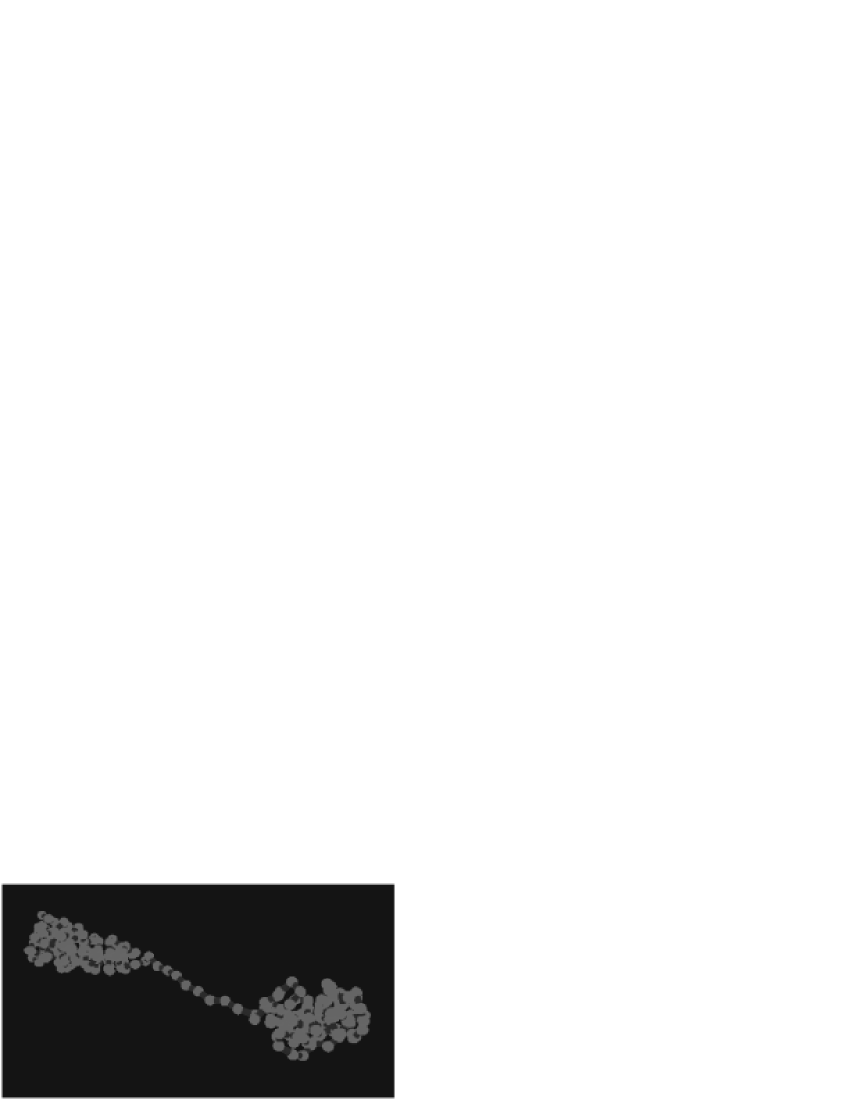
Figure 3: Molecular dynamics simulation of a $N=256$ polymer chain at temperature $T=3.0$, pearls regime at $t=4\times 10^{4}\Delta t$

Figure 4: Molecular dynamics simulation of a $N=256$ polymer chain at temperature $T=3.0$, globular state at $t=10^{5}\Delta t$

Figure 5: Molecular dynamics simulation of a $N=256$ polymer chain at temperature $T=0.1$, early stages of helix formation at $t=15\times 10^{4}\Delta t$

Figure 6: Molecular dynamics simulation of a $N=256$ polymer chain at temperature $T=0.1$, a well formed helix at $t=3\times 10^{5}\Delta t$

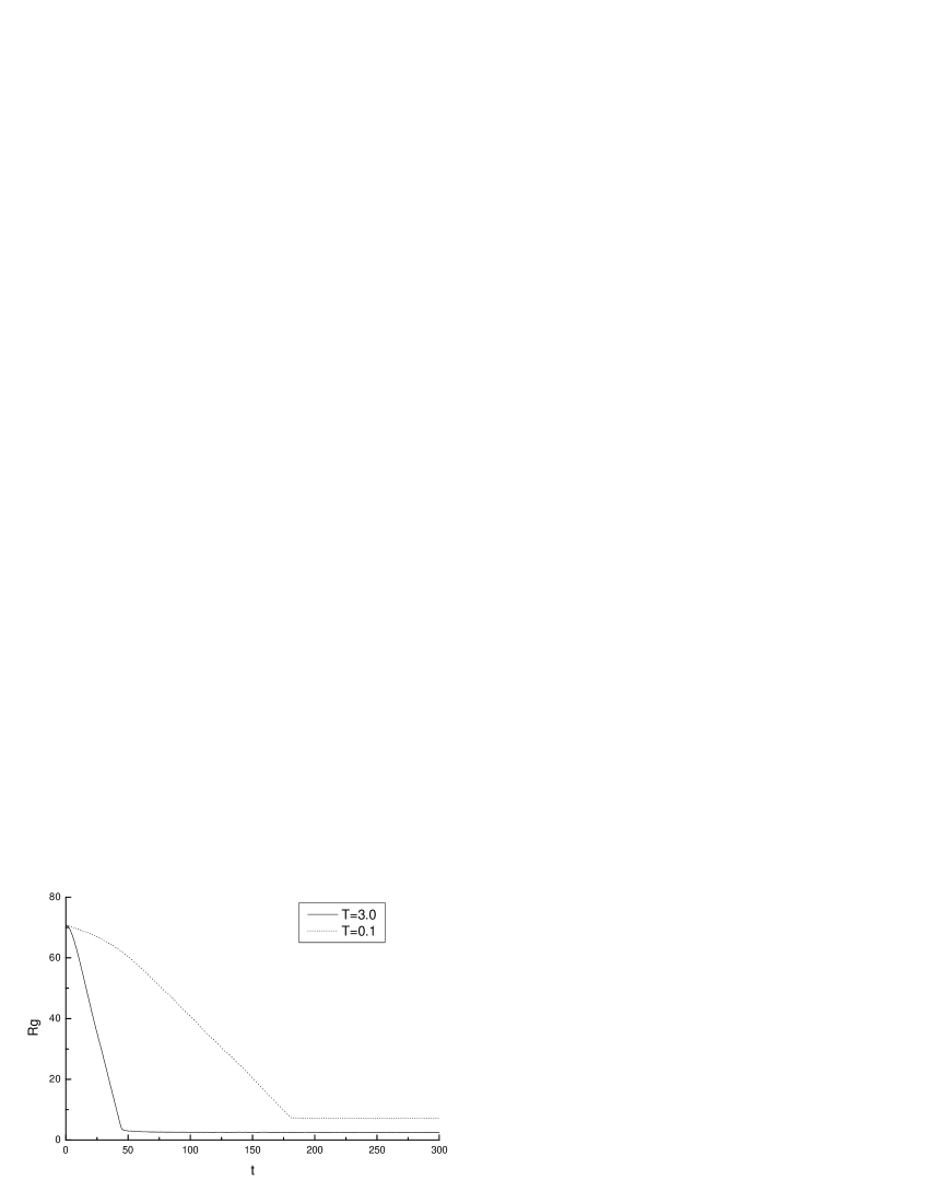
Figure 7: Gyration radius $R_{g}$ versus time for two differents temperatures $T=0.1$ and $T=3.0$ and polymer chain size $N=256$

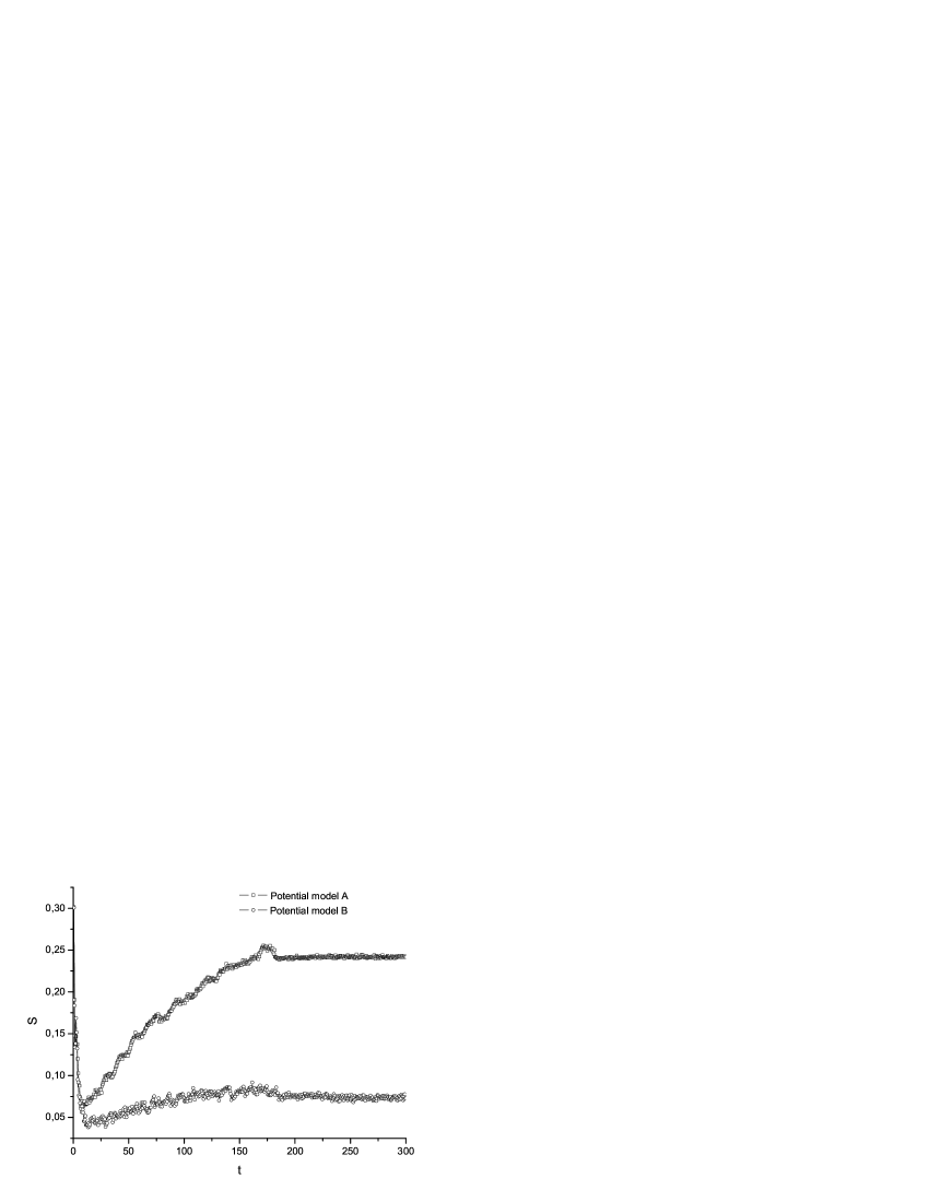
Figure 8: Order parameter as function of time for polymer chain size $N=256$ at temperature $T=0.1$ using potential model A and potential model B

Figure 9: Molecular dynamics simulation of a $N=128$ polymer chain at temperature $T=0.05$, a pair of helices with antiparallel alignement at $t=15\times 10^{4}\Delta t$

References

- [1] P.J Flory. Cornell University Press, Ithaca, (1967)
- [2] M.J. Stephen, Physics Letters, 53 A, 5 (1975)
- [3] P. G. de Gennes, Scaling Concepts in Polymer Physics Cornell,Ithaca, (1979)
- [4] P. G. de Gennes, J. Phys. Lett. 46, L-639 (1985)
- [5] J. B. Imbert, A. Lesne, and J. M. Victor Phys Rev E, 56, 5 (1997)
- [6] A. Michel and S. Kreitmeier, Comp. and Theo. Polymer Science 7, 113-120 (1997)
- [7] P. Rominszowski, A. Sikorski, Comp. and Theo. Polymer Science 11 129-131 (2001)
- [8] G.C Pereira, D.R.M. Williams, ANZIAM J., 45 (E) pp C163 C173, (2004)
- [9] B. Shnurr, F.C. MacKintosh and D.R.M. Williams Europhys. Lett, 51,3, pp. 279-285 (2000)
- [10] A. Montesi, M. Pasquali, and F.C. MacKintosh, Phy Rev E 69, 021916 (2004)
- [11] Frish and Verga, Phys Rev E, 65, 041801 (2002)
- [12] Frish and Verga, Phys Rev E, 66, 041807 (2002)
- [13] J. M. Polson, Phys Rev E, 60, 3 (1999)
- [14] J. M. Polson and Martin J. Zuckermann, J. Chem. Phys. 113, 3 (2000)
- [15] J. M. Polson and N. E. Moore, J. Chem. Phys. 122, 024905 (2005)
- [16] N. Kikuchi, J. F. Ryder, C. Pooley, and J. M. Yeomans (2005)
- [17] W. G. Hoover, Ann. Rev. Phys. Chem. 34: 103-27, (1983)
- [18] W. G. Hoover, Phys. Rev. A. 31, 3 (1985)
- [19] D. Frenkel and B. Smit, Understanding Molecular Simulations (Academic Press, 1996)
- [20] C. W. Yong and Julian H. R. Clarke, Juan J. Freire, Marvin Bishop J. Chem. Phys. 105 (21), (1996)
- [21] P. Grassberger, Phys. Rev. E. 56, 3682 (1997)
- [22] C. Clementi, A. Maritan and J.R. Banavar, Phys. Rev. Lett. 81, 15, (1998)
- [23] D. C. Rapaport, Phys. Rev. E. 66,011906 (2002)
- [24] D. C. Rapaport, Phys. Rev. E. 68,041801 (2003)
- [25] J. P. Kemp and Z. Y. Chen, Phys. Rev. Lett. 81, 18, (1998)
- [26] Wei Cao, Clay Bracken, Neville R. Kallenbach and Min Lu, Protein Sci., 13: 177-189 (2004)