On the possibility of an excitonic insulator at the semiconductor-semimetal transition

Abstract

We calculate the critical temperature below which an excitonic insulator exists at the pressure-induced semiconductor-semimetal transition. Our approach is based on an effective-mass model for valence and conduction band electrons interacting via a statically screened Coulomb potential. Assuming pressure to control the energy gap, we derive, in the spirit of a BEC-BCS crossover scenario, a set of equations which determines, as a function of the energy gap (pressure), the chemical potentials for the two bands, the screening wave number, and the critical temperature. We (i) show that in leading order the chemical potentials are not affected by the exciton states, (ii) verify that on the strong coupling (semiconductor) side the critical temperatures obtained from the linearized gap equation coincide with the transition temperatures for BEC of non-interacting bosons, (iii) demonstrate that mass asymmetry strongly suppresses BCS-type pairing, and (iv) discuss in the context of our theory recent experimental claims for exciton condensation in ${\rm TmSe_{0.45}Te_{0.55}}$.

I I. Introduction

More then four decades ago Mott Mott (1961) realized that a semimetal (SM) with a low density of free charge carriers is unstable against an insulating, semiconducting (SC) state, because the Coulomb interaction binds conduction band electrons and valence band holes to excitons. At around the same time, Knox Knox (1963) made the important observation that a SC whose energy gap is smaller then the exciton binding energy has to be unstable against the spontanous formation of excitons. Understood as a global instability, the pairing of electrons and holes is expected to lead to a macroscopic, phase coherent quantum state or condensate – the excitonic insulator (EI) – separating below a critical temperature the SC from the SM. Theoretically Keldysh and Kopaev (1964); des Cloizeaux (1965); Kozlov and Maksimov (1965, 1966a, 1966b); Jerome et al. (1967); Keldysh and Kozlov (1968); Halperin and Rice (1968); Kohn (1968), the instability should occur in any material which can be tuned from an indirect gap semiconductor to a semimetal, for instance, by applying pressure, uniform stress, or by optical pumping. Yet, experimental efforts to establish the EI in real compounds largely failed.

It is only until recently that detailed studies of the pressure-induced SC-SM transition in ${\rm TmSe_{0.45}Te_{0.55}}$ by Wachter and coworkers strongly suggested the existence of an EI Neuenschwander and Wachter (1990); Bucher et al. (1991); Wachter (2001); Wachter et al. (2004). In particular, the anomalous increase of the electrical resistivity in a narrow pressure range around 8 kbar indicated the appearance of a new phase below 250 K Neuenschwander and Wachter (1990); Bucher et al. (1991). Wachter and coworkers suggested that this new phase might be an “excitonic insulator”, and, assuming pressure to modify only the energy gap ${E_{g}}$, constructed a phase diagram for ${\rm TmSe_{0.45}Te_{0.55}}$ in the ${E_{g}-T}$ plane Bucher et al. (1991). Later they found in the same material a linear increase of the thermal diffusivity below 20 K and related this to a superfluid exciton state Wachter et al. (2004). Both excitonic phases are located on the SC side of the SC-SM transition in ${\rm TmSe_{0.45}Te_{0.55}}$.

In the present paper we perform the first theoretical analysis of these astonishing experimental findings, staying strictly within the bounds of the concept of an EI as a superfluid condensate of electron-hole pairs, similar to a condensate of Cooper pairs in a superconductor. (We exclusively use the acronym EI to denote this state and refer to condensation when electron-hole pairs enter this state.) In contrast to the early theoretical works des Cloizeaux (1965); Keldysh and Kopaev (1964); Kozlov and Maksimov (1965, 1966a, 1966b); Jerome et al. (1967); Keldysh and Kozlov (1968); Halperin and Rice (1968); Kohn (1968), we (i) self-consistently calculate the phase boundary of the EI, (ii) analyze the EI in the spirit of a BEC-BCS crossover, and (iii) investigate also the halo of the EI, that is, the region surrounding the EI on the SC side.

The creation of an exciton condensate is usually attempted by optical pumping of suitable semiconductor structures Littlewood et al. (2004). So far, without success. The main obstacle is the far-off-equilibrium situation caused by optical excitation. In contrast, pressure-induced generation of excitons occurs at thermal equilibrium, which is much more favorable for condensation. Semiconducting, pressure-sensitive mixed valence materials, such as ${\rm TmSe_{0.45}Te_{0.55}}$, offer therefore a very promising route towards exciton condensation. It is even conceivable to use this class of materials for implementing recent proposals of coherent transport across EI-SM junctions Rontani and Sham (2005); Wang et al. (2005). The validation of Wachter and coworkers’ experiments would thus have a tremendous impact on the field of exciton condensation.

The excitonic instability is driven by the Coulomb interaction leading to pairing of conduction band (CB) electrons with valence band (VB) holes. Of particular importance is therefore to self-consistently determine its weakening when the external parameter, for instance pressure, pushes the material from the SC side, with only a few thermally excited charge carriers available for screening, to the SM side, with a huge number of charge carriers. The strength of the Coulomb interaction determines on which side of the SC-SM transition the system is. As long as the Coulomb interaction is strong enough to support excitons, that is, as long as the exciton binding energy is positive, the material is on the SC side. The vanishing of the binding energy (Mott effect Mott (1961)) defines then the SC-SM transition.

Figure 1: Qualitative sketch of the phase boundary of an EI with equal band masses. (Adopted from Ref. Kohn (1968).)

Depending from which side of the SC-SM transition the EI is approached (see Fig. 1), the EI typifies either a Bose-Einstein (BE) condensate of tightly bound excitons (SC side) or a BCS condensate of loosely bound electron-hole pairs (SM side) Leggett (1980); Comte and Nozières (1982). A characteristic feature of BEC of excitons on the SC side is that formation of excitons and phase coherence (condensation) occur at different temperatures Comte and Nozières (1982); Nozières and Schmitt-Rink (1985). While excitons already exist below the temperature ${T_{M}}$ set by the Mott effect, the EI, understood as a genuine condensate of excitons, occurs only below the critical temperature ${T_{c}<T_{M}}$. Thus, on the SC side, the EI is embedded in a region containing excitons in addition to VB holes and CB electrons. We call this region halo. On the SM side, in contrast, Cooper-type electron-hole pairs form and condense at the same temperature ${T_{c}}$. The difference between an EI sitting, respectively, on the SC and SM side of the SC-SM transition has important consequences for the interpretation of the ${\rm TmSe_{0.45}Te_{0.55}}$ data.

After the seminal studies by Leggett Leggett (1980), Comte and Nozières Comte and Nozières (1982), and Nozières and Schmitt-Rink Nozières and Schmitt-Rink (1985), the transition from BE to BCS condensation has been extensively studied in the past, mostly with an eye on short-coherence length superconductors Drechsler and Zwerger (1992); Cote and Griffin (1993); Haussmann (1993); de Melo et al. (1993); Roepke (1994); Maly et al. (1999); Pieri et al. (2004), but also electron-hole gases in semiconductors Cote and Griffin (1988); Shumway and Ceperley (1999), and, more recently, trapped atomic Fermi gases Ohashi and Griffin (2002); Chen et al. (2005) have been analysed from this point of view. From these analytical and numerical investigations it is known that the transition from BE to BCS condensation is smooth. It is also known that diagrammatic approaches usually capture the crossover only when the BCS equation for the order parameter is augmented by an equation for the chemical potential. At zero temperature, it suffices to calculate both quantities in meanfield approximation Leggett (1980); Comte and Nozières (1982). At finite temperatures, however, the chemical potential has to be at least determined within a T-matrix approximation which accounts for the excitation of collective modes, i.e. in the context of an EI, of excitons with finite center-of-mass momentum Nozières and Schmitt-Rink (1985).

In order to discuss the EI at the pressure-induced SC-SM transition in terms of a BEC-BCS crossover, we need therefore not only equations for the order parameter and the screening wave number (to account for the Mott effect) but also for the CB electron and VB hole chemical potentials. Because pressure controls the chemical potentials, which in turn are constrained by charge neutrality, the meanfield approximation turns out, even for finite temperatures, to be sufficient on the (weak coupling) SM side and the (strong coupling) SC side, in contrast to what one would expect from related diagrammatic studies of the crossover problem in high-${T_{c}}$ materials and atomic Fermi gases Drechsler and Zwerger (1992); Haussmann (1993); de Melo et al. (1993); Maly et al. (1999); Pieri et al. (2004); Ohashi and Griffin (2002); Chen et al. (2005). Using the Thouless criterion Thouless (1960) (see also Keldysh and Kozlov (1968)) to determine the transition temperature for BEC directly from the normal phase electron-hole T-matrix, we verify that the transition temperatures obtained from the meanfield equations indeed coincide on the SC side with the transition temperatures for BEC of non-interacting bosonic excitons. From the normal phase electron-hole T-matrix we furthermore extract the temperature ${T_{M}}$ above which excitons cease to exist and construct a mass-action-law to determine the composition of the EI’s halo.

As far as Wachter and coworkers’ experiments Neuenschwander and Wachter (1990); Bucher et al. (1991); Wachter (2001); Wachter et al. (2004) are concerned we come to the following conclusions. The phase boundary constructed from the resistivity data does not embrace the EI. Instead, it most probably reflects that part of the halo of the EI where excitons prevail over free electrons and holes and give rise to an efficient additional scattering channel which leads to the observed resistivity anomaly. More remarkable is however that from our theoretical results we would expect the EI – that is, the macroscopic, phase coherent condensate – exactly in the temperature range where the linear increase of the thermal diffusivity was observed Wachter et al. (2004). In analogy to liquid He 4, Wachter and coworkers suggest that the increase could be due to the second sound of a superfluid exciton liquid. We, on the other hand, find the EI entirely on the SC side, where, within our approximations, it constitutes a BEC of ideal bosonic excitons. The BCS side of the EI, where it is unclear whether superfluidity can be realized Kozlov and Maksimov (1966b) or not Zittartz (1968), is strongly suppressed for finite temperatures because of the large asymmetry between the CB and VB masses in ${\rm TmSe_{0.45}Te_{0.55}}$. Of course, an ideal gas of bosons cannot become superfluid and thus cannot feature a second sound. In reality, however, excitons interact and could, when the interaction is dominantly repulsive, give rise to it. Thus, Wachter and coworkers Wachter et al. (2004) may have seen an exciton condensate.

In the next section we first introduce an effective-mass model on which our calculation is based and then give a description of our calculational scheme. In section III we present numerical results for the phase boundary ${T_{c}(E_{g})}$ of the EI, first for equal band masses, where we obtain a steeple-like ${T_{c}(E_{g})}$, directly reflecting the different condensation mechanisms on the SC and SM side, and then for asymmetric band masses, applicable to Tm[Se,Te] compounds, where we find a strongly suppressed ${T_{c}(E_{g})}$ on the SM side and thus an EI sitting almost entirely on the SC side of the SC-SM transition. We then relate in section IV our results to the experimental data for the pressure induced SC-SM transition in ${\rm TmSe_{0.45}Te_{0.55}}$ and conclude in section V.

II II. Formalism

II.1 A. Model

The excitonic instability arises because of the Coulomb attraction between electrons in the lowest CB ($i=1$) and holes in the highest VB ($i=2$), with an indirect energy gap separating the two bands. Since the spin algebra would unnecessarily mask the many-body theoretical concepts we want to discuss, we focus on spinless fermions. Only in section III, where we make contact with experiments, we include the spin in our calculation.

Keeping only the dominant term of the Coulomb interaction, which we assume to be statically screened, an effective-mass model for studying the (spinless) Wannier-type EI is

$$H=\sum_{{\bf k},i}{e}_{i}({\bf k})c_{i,{\bf k}}^{\dagger}c_{i,{\bf k}}+\frac{1}{2}\sum_{{\bf q}}V_{s}({\bf q})\rho({\bf q})\rho(-{\bf q}),$$ (1)

with $\rho({\bf q})=\sum_{i,{\bf k}}c_{i,{\bf k}+{\bf q}}^{\dagger}c_{i,{\bf k}}$ the total charge density and $V_{s}({\bf q})=(4\pi e^{2}/\epsilon_{0})/(q^{2}+q_{s}^{2})$. The screening wave number $q_{s}$ depends on the CB electron and VB hole density and will be determined self-consistently in the course of the calculation; $\epsilon_{0}$ is the background dielectric constant. The momenta ${\bf k}$ for CB electrons and VB holes are measured from the respective extrema of the bands which are separated by half of a reciprocal lattice vector ${\bf w}={\bf K}/2$. We consider the case where both the VB and the CB band have one extremum. Assuming isotropic effective masses $m_{i}$, the band dispersions read ($\hbar=1$ throughout the paper)

$${e}_{1}({\bf k})={E_{g}}+\varepsilon_{1}({\bf k})-\mu,~{}~{}\\ {e}_{2}({\bf k})=-\varepsilon_{2}({\bf k})-\mu-\Sigma_{0}({\bf k}),$$ (2)

with $\varepsilon_{i}({\bf k})={\bf k}^{2}/2m_{i}$, ${E_{g}}$ the bare energy gap which can be varied continuously through zero under pressure, and $\mu$ the chemical potential. The band structure (2) refers to the unexcited crystal at ${T=0}$ with an empty CB and a full VB whose selfenergy $\Sigma_{0}({\bf k})$ has to be subtracted Zimmermann (1976).

For model (1) to be applicable for the description of an EI we have to assume that through the SC-SM transition all parameters, except the energy gap ${E_{g}}$ and the screening wave number $q_{s}$, vary weakly and can be kept constant. Since model (1) treats an indirect gap semiconductor as a direct gap semiconductor, effects due to the indirect gap Halperin and Rice (1968), in particular, multi-valley effects (when the valleys are not identical) and the balancing of the finite momentum ${\bf w}$ of the electron-hole pairs by the lattice leading, for instance, to (small) density modulations in the EI phase are beyond the scope of the present paper.

II.2 B. Meanfield approximation

In formal analogy to the theory of superconductivity, we employ matrix propagators (in the band indices $i=1,2$)

$${G}_{ij}({\bf k},\tau)=-\langle{T}_{\tau}c_{{\bf k},i}(\tau)c_{{\bf k},j}^{\dagger}(0)\rangle,$$ (3)

with $0\leq\tau\leq\beta$ and ${T}_{\tau}[...]$ the time-ordering operator with respect to $\tau$. The diagonal elements ${G}_{ii}$ denote the (normal) propagators for electrons in the CB and VB, respectively, whereas the off-diagonal (anomalous) propagators describe the phase coherence of electron-hole pairs. Finite anomalous propagators signal the condensate and thus the EI.

In Matsubara space, the matrix propagator satisfies a Dyson equation,

$${G}(k)={g}(k)+{g}(k)\Sigma(k){G}(k),$$ (4)

with a diagonal matrix

$${g}_{ij}(k)=[i\omega_{n}-{e}_{i}({\bf k}]^{-1}\delta_{ij},$$ (5)

denoting the bare propagator and a 2$\times$2 selfenergy matrix $\Sigma$, which we assume to be given by a skeleton expansion, that is, in terms of the fully dressed propagator ${G}$. The variable $k=({\bf k},i\omega_{n})$ denotes a four-vector with ${\bf k}$ a momentum and $\omega_{n}=(2n+1)\pi/\beta$ ($n$ integer) a fermionic Matsubara frequency.

Separating the selfenergy into diagonal (normal) and off-diagonal (anomalous) parts and suppressing the $k$ dependence, we rewrite the Dyson equation as

$${G} = {\cal G}+{\cal G}\Sigma^{A}{G},$$ (6)

$${\cal G} = {g}+{g}\Sigma^{N}{\cal G}$$ (7)

with $\Sigma^{A}$ and $\Sigma^{N}$ the anomalous and normal selfenergy, respectively.

The separation of the Dyson equation is particularly useful for the calculation of the transition temperature ${T_{c}}$. We first note from Eq. (7) that ${\cal G}$ is diagonal. Thus, Eq. (6) reduces to

$${G}^{-1}=\bigg{(}\begin{array}[]{cc}{\cal G}_{11}^{-1}-{\cal G}_{22}|\Sigma^{A}_{12}|^{2}&\big{[}{\cal G}_{11}{G}_{22}\Sigma^{A}_{12}\big{]}^{-1}\\ \big{[}{\cal G}_{22}{G}_{11}\Sigma^{A}_{21}\big{]}^{-1}&{\cal G}_{22}^{-1}-{\cal G}_{11}|\Sigma^{A}_{12}|^{2}\end{array}\bigg{)}.$$ (10)

In the vicinity of the transition temperature ${T_{c}}$ the anomalous selfenergy becomes vanishingly small and Eq. (10) can be linearized with respect to $\Sigma^{A}$. The anomalous propagator ${G}_{12}$ is then given by

$${G}_{12} = {\cal G}_{11}{\cal G}_{22}\Sigma^{A}_{12},$$ (11)

where the propagators ${\cal G}_{ii}$ satisfy Eq. (7) with $\Sigma^{N}$ calculated from ${\cal G}_{ii}$ alone; ${G}_{12}$ and ${G}_{21}$ do not enter $\Sigma^{N}$ anymore. Thus, within the linearized theory, the calculation of the normal propagators is decoupled from the calculation of the anomalous propagators. From Eq. (11), we see moreover that ${G}_{12}\neq 0$ is equivalent to $\Sigma^{A}_{12}\neq 0$. Accordingly, the anomalous selfenergy can be considered as an order parameter.

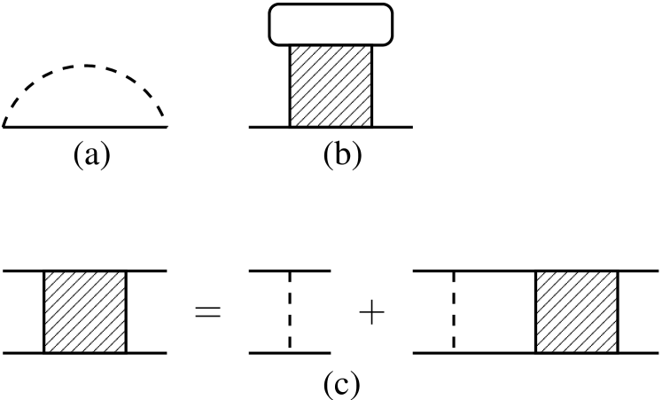
Figure 2: (a) exchange selfenergy $\Sigma^{X}$ to be used in the meanfield approximation, (b) ladder selfenergy $\Sigma^{L}$ additionally used in the T-matrix approximation, and (c) ladder equation for the T-matrix. Solid (dashed) lines denote matrix propagators (statically screened Coulomb potentials).

To proceed we have to specify the selfenergies $\Sigma^{N}$ and $\Sigma^{A}$. In the meanfield approximation both are given by the exchange energy $\Sigma^{X}$ shown in Fig. 2a. Applying standard diagrammatic rules Schrieffer (1964), we find

$$\Sigma^{X}_{ii}({\bf k})=-\int\frac{d{\bf k^{\prime}}}{(2\pi)^{3}}V_{s}({\bf k-k^{\prime}})n_{\rm F}(\bar{e}_{i}({\bf k^{\prime}})$$ (12)

for the normal selfenergies and

$$\Delta({\bf k})=\int\frac{d{\bf k^{\prime}}}{(2\pi)^{3}}V_{s}({\bf k-k^{\prime}})Q({\bf k^{\prime}})\Delta({\bf k^{\prime}})$$ (13)

with

$$Q({\bf k})=\frac{n_{\rm F}(\bar{e}_{2}({\bf k}))-n_{\rm F}(\bar{e}_{1}({\bf k}))}{\bar{e}_{1}({\bf k})-\bar{e}_{2}({\bf k})}$$ (14)

for the anomalous selfenergy $\Delta({\bf k})=\Sigma^{X}_{12}({\bf k})$, where $n_{\rm F}$ denotes the Fermi function.

Note, the normal selfenergies contain no Coulomb-hole term because we replaced directly in the Hamiltonian the bare Coulomb interaction by the statically screened one (static screening approximation); the correlation energy is thus partly suppressed. As a consequence, excitonic phases are energetically more favorable than electron-hole liquid phases Rice (1977), independent of the mass ratio and the number of valleys, and in contrast to, for instance, what one finds in the quasi-static approximation Bronold et al. , which performs the replacement (with a modified screened Coulomb potential) after the selfenergies have been calculated in the random-phase approximation Haug and Schmitt-Rink (1984). Neither approximation, however, should be used to study the competition between the two phases, because both do not give a reliable correlation energy for intermediate densities, that is, close to the SC-SM transition, where excitons should be included in the correlation energy Roepke and Der (1979). In addition, scattering processes beyond our model, for instance, between valleys or with phonons, also affect the competition between excitonic and electron-hole liquid phases. An investigation of the competition between the two is thus a complex task, beyond the scope of the present paper, which simply assumes excitons to be favored from the start. The static screening model is thus sufficient.

The single particle energies entering Eqs. (12) and (14) are the self-consistent solutions of

$${\bar{e}_{i}}({\bf k})={e}_{i}({\bf k})+\Sigma^{X}_{ii}({\bf k}).$$ (15)

The main effect of the exchange energy on the particle dispersions is a rigid, ${\bf k}$-independent energy shift which we incorporate into chemical potentials for the CB electrons and VB holes. Writing the renormalized dispersions as

$${\bar{e}_{i}}({\bf k})=(-1)^{i+1}(\varepsilon_{i}({\bf k})-\mu_{i})$$ (16)

yields for the electron and hole chemical potentials

$$\mu_{1} = \mu-{E_{g}}-\Delta{e}_{1},$$ (17)

$$\mu_{2} = \Delta{e}_{2}-\mu,$$ (18)

with energy shifts satisfying

$$\Delta{e}_{i}=(-1)^{i}\int\frac{d{\bf k}}{(2\pi)^{3}}V_{s}({\bf k})n_{\rm F}(\varepsilon_{i}({\bf k})-\mu_{i}).$$ (19)

To derive Eq. (19) for $i=2$, the selfenergy $\Sigma_{0}$ of the full VB has to be calculated within the same approximation and then drops out. Together with Eq. (19), Eqs. (17) and (18) effectively define an electron-hole representation which is convenient for the calculation of the screening parameter $q_{s}$.

In order to obtain a closed set of equations for the three unknown parameters $\mu$, $\mu_{1}$, and $\mu_{2}$, we augment Eqs. (17) and (18) by the condition of charge neutrality which forces CB electron and VB hole densities, given in the meanfield approximation, respectively, by

$$n_{1} = \int\frac{d{\bf k}}{(2\pi)^{3}}n_{\rm F}(\varepsilon_{1}({\bf k})-\mu_{1}),$$ (20)

$$\bar{n}_{2} = \int\frac{d{\bf k}}{(2\pi)^{3}}n_{\rm F}(\varepsilon_{2}({\bf k})-\mu_{2}),$$ (21)

to be equal. Thus, charge neutrality leads to the constraint

$$\int\frac{d{\bf k}}{(2\pi)^{3}}\left[n_{\rm F}(\varepsilon_{1}({\bf k})-\mu_{1})-n_{\rm F}(\varepsilon_{2}({\bf k})-\mu_{2})\right]=0,$$ (22)

which we use to eliminate $\mu$ in Eqs. (17) and (18). For that purpose, we add Eqs. (17) and (18)

$$\mu_{1}+\mu_{2}=-{E_{g}}+\sum_{i}\int\frac{d{\bf k}}{(2\pi)^{3}}V_{s}({\bf k})n_{\rm F}(\varepsilon_{i}({\bf k})-\mu_{i})$$ (23)

and combine this equation with the charge neutrality constraint (22). Physically, the sum of the CB electron and VB hole chemical potentials is the negative of the renormalized energy gap:

$$\bar{E}_{g}=\bar{e}_{1}(0)-\bar{e}_{2}(0)=-\mu_{1}-\mu_{2}.$$ (24)

With the individual chemical potentials for each species at our disposal, the screening parameter $q_{s}$ is given by

$$q_{s}^{2}=\frac{4\pi e^{2}}{\epsilon_{0}}\left(\frac{\partial}{\partial\mu_{1}}n_{1}+\frac{\partial}{\partial\mu_{2}}\bar{n}_{2}\right).$$ (25)

Once $\mu_{1},\mu_{2}$, and $q_{s}^{2}$ are calculated, the kernel of the gap equation (13) is known in the whole ${E_{g}-T}$ plane. For a given energy gap ${E_{g}}$, we can thus determine the transition temperature ${T_{c}}$ as the highest temperature for which the homogeneous integral equation (13) has a nontrivial solution $\Delta({\bf k})\neq 0$.

II.3 C. T-matrix approximation

The meanfield theory presented in the previous subsection determines ${T_{c}(E_{g}})$ on the strong coupling (SC) as well as on the weak coupling (SM) side. The transition temperatures on the SC side turn out to coincide with the BEC transition temperatures for a non-interacting boson gas of excitons (see section III), as it should Keldysh and Kozlov (1968); Nozières and Schmitt-Rink (1985). From the perspective of diagrammatic BEC-BCS crossover theories Nozières and Schmitt-Rink (1985); Drechsler and Zwerger (1992); Haussmann (1993); de Melo et al. (1993); Maly et al. (1999); Pieri et al. (2004); Ohashi and Griffin (2002); Chen et al. (2005) this is however surprising because the meanfield theory does not account for excitons existing on the SC side already above the transition temperature ${T_{c}(E_{g}})$. These excitons are expected to at least modify the chemical potentials $\mu_{i}$. However, the charge neutrality constraint, inherent in a pressure-driven BEC-BCS crossover, leads to a cancellation of the leading order corrections to the chemical potentials.

Diagrammatic BEC-BCS crossover theories Nozières and Schmitt-Rink (1985); Drechsler and Zwerger (1992); Haussmann (1993); de Melo et al. (1993); Maly et al. (1999); Pieri et al. (2004); Ohashi and Griffin (2002); Chen et al. (2005) usually leave the gap equation (13) unchanged but calculate the charge densities from normal propagators dressed not only with the exchange selfenergy $\Sigma^{X}$ (Fig. 2a) but also with the ladder selfenergy $\Sigma^{L}$ (Fig. 2b), which takes, via the electron-hole T-matrix (Fig. 2c), normal phase excitons into account. Expanding the spectral functions to which the total selfenergy gives rise to with respect to the imaginary part of $\Sigma^{L}$ Zimmermann and Stolz (1985) (see appendix A), the CB electron (VB hole) density can be written as $n_{1}=n_{1}^{f}+n_{1}^{b}$ ($\bar{n}_{2}=\bar{n}_{2}^{f}+\bar{n}_{2}^{b}$) with the superscripts ‘f’ and ‘b’ denoting, respectively, the part of the total density coming from free electrons (holes), with a modified dispersion but a spectral weight unity, and the part arising from bound electron-hole pairs. The charge neutrality condition (22) becomes therefore $n_{1}^{f}+n_{1}^{b}=\bar{n}_{2}^{f}+\bar{n}_{2}^{b}$. Now it is important to realize (or to verify by calculation, see appendix A) that whenever a CB electron participates in an exciton, a VB hole has to do the same. Thus, $n_{1}^{b}=\bar{n}_{2}^{b}$, and the charge neutrality condition reduces to $n_{1}^{f}=\bar{n}_{2}^{f}$ which, except for the modifications of the dispersions due to $\Sigma^{L}$ has the same form as in the meanfield approximation.

The above argument is independent from the approximation used to obtain the electron-hole T-matrix. It is only based on charge neutrality and the fact that an exciton has to contain both an electron and a hole. The calculation shows that it is crucial to employ the skeleton expansion. As a result, the single particle dispersions are modified by $\Sigma^{L}$ and thus by excitons (see Eq. (47)). The ladder approximation (Fig. 2c) we use to calculate the T-matrix does however not consistently account for feedback effects of this kind; for that purpose, additional diagrams Roepke (1994) or a systematic mode-coupling approach Cote and Griffin (1988, 1993) should be implemented. We consider therefore feedback of excitons to single particle states as higher order effects and ignore all of them, including the one already present in the ladder approximation. The charge neutrality condition in the ladder approximation reduces then to the meanfield charge neutrality condition. Note, feedback effects induce interactions between pairs Pieri et al. (2004). Neglecting them implies therefore to stay within the framework of a non-interacting, ideal gas of excitons. How to extract from the skeleton expansion (and not from an algebraic mapping which is questionable in the vicinity of the SC-SM transition) the interaction between electron-hole pairs, which not only contains the repulsive core at short distances because of the Pauli exclusion but also the weakly attractive tail at large distances, is to the best of our knowledge an unsolved problem and beyond the scope of the present paper.

In appendix A we calculate the charge densities within the ladder approximation shown in Fig. 2 using the separable approximation for the normal phase electron-hole T-matrix described in appendix B. Thereby, we proof by calculation that $n_{1}=\bar{n}_{2}$ reduces to $n_{1}^{f}=\bar{n}_{2}^{f}$. Because the screening parameter $q_{s}$, on the other hand, accounts only for screening due to free charge carriers it has to be calculated from $n_{1}^{f}$ and $\bar{n}_{2}^{f}$. Thus, even for finite temperatures, the meanfield approximation of the previous subsection is on par with T-matrix based BEC-BCS crossover theories Nozières and Schmitt-Rink (1985); Drechsler and Zwerger (1992); Haussmann (1993); de Melo et al. (1993); Maly et al. (1999); Pieri et al. (2004); Ohashi and Griffin (2002); Chen et al. (2005).

As an additional check, we now deduce the transition temperature on the SC side directly from the normal phase electron-hole T-matrix (which takes excitons with finite center-of-mass momentum into account) using the Thouless criterion Thouless (1960) (see also Keldysh and Kozlov (1968)) and verify that the ${T_{c}(E_{g})}$ calculated within the meanfield approximation indeed coincides with the transition temperatures obtained from the T-matrix. Thereby, we also verify that the neglect of the feedback of excitons on single particle states leads to a non-interacting bosonic gas of excitons.

In the approximation depicted in Fig. 2c, the normal phase electron-hole T-matrix is given by

$$\Lambda_{12}({\bf k},{\bf k^{\prime}};{\bf q},i\Omega_{n})=V_{s}({\bf k-k^{\prime}})+\int\frac{d{\bf k^{\prime\prime}}}{(2\pi)^{3}}V_{s}({\bf k-k^{\prime\prime}})Q({\bf k^{\prime\prime}};{\bf q},i\Omega_{n})\Lambda_{12}({\bf k^{\prime\prime}},{\bf k^{\prime}};{\bf q},i\Omega_{n})$$ (26)

with an electron-hole pair propagator

$$Q({\bf k};{\bf q},i\Omega_{n})=\frac{1-n_{\rm F}(\varepsilon_{1}({\bf k})-\mu_{1})-n_{\rm F}(\varepsilon_{2}({\bf k}-{\bf q})-\mu_{2})}{\bar{E}_{g}+\varepsilon_{1}({\bf k})+\varepsilon_{2}({\bf k}-{\bf q})-i\Omega_{n}}.$$ (27)

Here, we used Eq. (16) to express renormalized dispersions $\bar{e}_{i}$ in terms of chemical potentials $\mu_{i}$ and definition (24) to introduce the renormalized energy gap; $\Omega_{n}=2n\pi/\beta$ ($n$ integer) are bosonic Matsubara frequencies and ${\bf q}$ denotes the center-of-mass momentum of an electron-hole pair (and thus of an exciton).

Taking advantage of the fact that the most important part of the normal phase electron-hole T-matrix originates form the exciton state, we calculate in appendix B the T-matrix within a separable approximation. As a result, we obtain

$$\Lambda_{12}({\bf k},{\bf k^{\prime}};{\bf q},i\Omega_{n})=g(|{\bf k}-\frac{m_{1}}{M}{\bf q}|)\cdot D_{X}({\bf q},i\Omega_{n}-\bar{E}_{g}-\frac{q^{2}}{2M})\cdot g(|{\bf k^{\prime}}-\frac{m_{1}}{M}{\bf q}|)$$ (28)

with a renormalized exciton propagator

$$D_{X}({\bf q},i\Omega_{n})=\frac{-1}{i\Omega_{n}+B+M_{X}({\bf q},i\Omega_{n})}$$ (29)

and form factors

$$g(p)=\int_{0}^{\infty}\frac{dp^{\prime}p^{\prime 2}}{4\pi^{2}}V_{s}(p,p^{\prime})\chi(p^{\prime})=\bigg{[}\frac{p^{2}}{2m}+B\bigg{]}\chi(p)$$ (30)

defined in terms of a screened exciton wavefunction $\chi$ and a screened exciton binding energy $B$ (see below and appendix B). Here, $V_{s}(p,p^{\prime})$ denotes the screened Coulomb potential averaged over the angle between ${\bf p}$ and ${\bf p^{\prime}}$, $M=m_{1}+m_{2}$ is the total mass, and $m=m_{1}m_{2}/M$ is the reduced mass of an electron-hole pair.

The exciton propagator (29) describes an exciton in a medium consisting of a finite density of CB electrons and VB holes. The screened exciton binding energy $B$ already accounts for the screening due to spectator particles not participating in the exciton. The spectators’ Pauli blocking, on the other hand, is included through the selfenergy

$$M_{X}({\bf q},i\Omega_{n})=-\int\frac{d{\bf p}}{(2\pi)^{3}}\frac{[\frac{p^{2}}{2m}+B]^{2}}{\frac{p^{2}}{2m}-i\Omega_{n}}\chi^{2}(p)\bigg{[}n_{\rm F}(\varepsilon_{1}({\bf p}+\frac{m_{1}}{M}{\bf q})-\mu_{1})+n_{\rm F}(\varepsilon_{2}({\bf p}-\frac{m_{2}}{M}{\bf q})-\mu_{2})\bigg{]}.$$ (31)

To avoid unnecessary numerical work, we replace in Eq. (30) the statically screened Coulomb potential by the Hulthen potential Haug and Koch (1993),

$$V_{s}(r)=\frac{e^{2}}{\epsilon_{0}}\frac{\exp{(-q_{s}r)}}{r}\rightarrow V_{H}(r)=\frac{e^{2}}{\epsilon_{0}}\frac{2q_{s}}{\exp{(2q_{s}r)}-1},$$ (32)

which is a good approximation as long as the screening wave number $q_{s}$ is not too large. Indeed, in the limit $q_{s}\rightarrow 0$, the Hulthen potential reduces to the unscreened Coulomb potential. With the replacement (32), Eq. (30) can be solved analytically Haug and Koch (1993). The screened exciton wavefunction and the screened exciton binding energy for $a_{X}\cdot q_{s}<1$ are, respectively, given by

$$\chi(p) = \frac{8\sqrt{\pi a_{X}^{3}(1-(a_{X}\cdot q_{s})^{2})}}{[(1-a_{X}\cdot q_{s})^{2}+(a_{X}\cdot p)^{2}]\cdot[(1+a_{X}\cdot q_{s})^{2}+(a_{X}\cdot p)^{2}]},$$ (33)

$$B = R_{X}(1-a_{X}\cdot q_{s})^{2},$$ (34)

where $R_{X}=1/2ma_{X}^{2}$ is the exciton Rydberg and $a_{X}=\epsilon_{0}/me^{2}$ is the exciton Bohr radius ($e$ bare electron charge). For $a_{X}\cdot q_{s}>1$, the Hulthen potential does not support a bound state and we have to set $\chi=B=0$ in that parameter range. Notice, in the limit $q_{s}\rightarrow 0$, Eqs. (33) and (34), respectively, reduce to the wave function and binding energy of an isolated exciton (no medium effects) as obtained from Eq. (30) with $V_{s}$ replaced by the angle averaged unscreened Coulomb potential.

The pole of the exciton propagator (29) determines the analytical structure of the T-matrix. Physically, it gives the exciton binding energy $\bar{B}({\bf q})$ renormalized by screening and phase space filling. Assuming a weak ${\bf q}$-dependence, $\bar{B}({\bf q})\approx\bar{B}(0)\equiv\bar{B}$, with the renormalized exciton binding energy $\bar{B}$ determined from

$$\bar{B}=B+{\rm Re}M_{X}(0,i\Omega_{n}\rightarrow-\bar{B}+i\eta).$$ (35)

In terms of $\bar{B}$ the exciton propagator can be rewritten as

$$D_{X}({\bf q},i\Omega_{n})=\frac{-Z_{X}}{i\Omega_{n}+\bar{B}}$$ (36)

with an exciton spectral weight defined by

$$Z_{X}=1-\frac{\partial}{\partial\Omega}{\rm Re}M_{X}(0,\Omega+i\eta)|_{\Omega=-\bar{B}}.$$ (37)

The Thouless criterion states that BEC of excitons occurs when the normal phase electron-hole T-matrix diverges at ${\bf q}=0$ and $i\Omega_{n}=0$. Using Eq. (28) this implies $D_{X}^{-1}(0,-\bar{E}_{g})=0$. With Eq. (36), the transition temperature ${T_{c}}({E_{g}})$ is thus given by

$$\bar{B}({E}_{g},{T_{c}})=\bar{E}_{g}({E}_{g},{T_{c}}),$$ (38)

where we displayed the dependence of the renormalized binding energy and the renormalized energy gap on the bare energy gap and the temperature.

In order to make the physical content of Eq. (38) more transparent, we rewrite it in terms of chemical potentials. Recalling the definition (24) of the renormalized energy gap, Eq. (38) becomes

$$\mu_{X}=\mu_{1}+\mu_{2}=-\bar{B},$$ (39)

which is equivalent to the criterion for BEC of a non-interacting Bose gas: The transition occurs when the chemical potential $\mu_{X}$ of the bosons reaches the bottom of the boson band leading to a macroscopic occupation of the ${\bf q}=0$ state.

The Thouless criterion per se Thouless (1960) can be used to determine ${T_{c}}({E_{g}})$ on the SC Keldysh and Kozlov (1968) and the SM Kozlov and Maksimov (1965) side. However, by construction, Eq. (28) describes the normal phase electron-hole T-matrix only on the SC side, where excitons exist, and the separable approximation for the T-matrix is applicable. Thus, we can use the Thouless criterion only on the SC side.

The exciton binding energy obtained from Eq. (35) enables us also to determine the phase boundary ${T_{M}}({E_{g}})$ between the SC and the SM and thus the halo of the EI, that is, the region between ${T_{M}}({E_{g}})$ and ${T_{c}}({E_{g}})$ on the SC side, where excitons, CB electrons and VB holes coexist. As originally suggested by Mott Mott (1961), we use the vanishing of $\bar{B}$ (Mott effect) as a criterion for the SC-SM transition. Accordingly, ${T_{M}}({E_{g}})$ is given by

$$\bar{B}({E_{g}},{T_{M}})=0.$$ (40)

III III. Results

To construct the phase boundary of the EI, we discretize the gap equation (13), and determine, for a given energy gap ${E_{g}}$, the temperature ${T_{c}}({E_{g}})$ for which the determinant of the coefficient matrix of the resulting linear set of equations vanishes. For each pair (${E_{g}},T$) we supply the chemical potentials $\mu_{1}$ and $\mu_{2}$ together with the screening wave number $q_{s}$ by finding the simultaneous roots of Eqs. (22), (23), and (25). To obtain the SC-SM phase boundary, we first determine, from Eq. (35), the renormalized exciton binding energy $\bar{B}$ as a function of ${E_{g}}$ and $T$, again providing for each pair (${E_{g}},T$) the chemical potentials and the screening wave number. After that, we search for a given ${E_{g}}$ for the temperature ${T_{M}}({E_{g}})$ which satisfies Eq. (40). In a similar way, we determine on the SC side, as a cross-check of the results obtained from the linearized gap equation, the critical temperature ${T_{c}}({E_{g}})$ from the Thouless criterion (38).

We consider an isotropic system, angles can be thus integrated analytically. All integrals over the magnitude of the momentum are done by Gaussian integration except the $|{\bf k}|$-integration appearing in the gap equation, which we perform by product integration, with the angle averaged Coulomb potential $V_{s}(k,k^{\prime})$ as the weight function. The logarithmic singularity of the kernel at $k=k^{\prime}$, which arises on the SC side for ${T}\rightarrow 0$, can thus be handled without problems. Recall, the separable approximation for the electron-hole T-matrix, on which the calculation of the renormalized exciton binding energy $\bar{B}$ is based, uses the Hulthen potential instead of the statically screened Coulomb potential. All results are presented in exciton units, measuring energies and temperatures in exciton Rydbergs $R_{X}$ and lengths in exciton Bohr radii $a_{X}$.

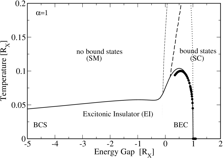
Figure 3: Phase boundary of an EI with equal band masses ($\alpha=m_{1}/m_{2}=1)$. The solid line (full circle) denotes the critical temperature obtained from the linearized gap equation (Thouless criterion for BEC). The dotted line shows part of the phase boundary on the SC side when no screening due to thermally excited charge carriers is taken into account. The thick (thin) dashed line indicates the SC-SM transition, defined by the vanishing of the renormalized (screened) binding energy, taking screening and Pauli blocking (only screening) into account.

The phase boundary ${T_{c}}({E_{g}})$ for an EI with equal band masses ($\alpha=m_{1}/m_{2}=1$) is presented in Fig. 3. The solid line shows ${T_{c}(E_{g})}$ obtained from the linearized gap equation (13). The solid circles on the SC side, on the other hand, give the ${T_{c}(E_{g})}$ deduced from the Thouless criterion (38) for BEC. The two critical temperatures coincide almost perfectly supporting our claim that even for finite temperatures the meanfield theory captures BEC on the SC side. The small deviations between the two curves as we come closer to the SC-SM transition (thick dashed line) originate from the discrepancy between the Hulthen and the screened Coulomb potential when the screening wave number increases.

From Fig. 3 we see that above $T\approx 0.12$ the EI is unstable and an ordinary SC-SM transition occurs (thick dashed line), here defined by the vanishing of the renormalized exciton binding energy $\bar{B}$. For $T<0.12$, we find a steeple-like phase boundary, which strongly discriminates between ${E_{g}}>0$ and ${E_{g}}<0$. For ${E_{g}}>0$, ${T_{c}}({E_{g}}$) first increases rather rapidly with increasing ${E_{g}}$, reaches a maximum, and then decreases to zero at ${E_{g}}=1$, the critical energy gap, above which the EI cannot exist Keldysh and Kopaev (1964); des Cloizeaux (1965); Kozlov and Maksimov (1965); Jerome et al. (1967); Halperin and Rice (1968). For ${E_{g}}<0$, in contrast, ${T_{c}(E_{g})}$ initially drops relatively fast, stays almost constant in a narrow ${E_{g}}$-range, and then decreases monotonously with further decreasing ${E_{g}}$. Notice, in contrast to the qualitative phase boundary of Fig. 1, the calculated ${T_{c}(E_{g})}$ reaches the BCS asymptotics only at very large band overlaps, far away from the SC-SM transition. On the scale of the exciton binding energy, we find no simple exponential dependence of the transition temperature on the band overlap $|E_{g}|$.

The steeple-like shape of the phase boundary reflects the different character of the EI when it is approached from the SM and the SC side, respectively. Deep on the SM side ($E_{g}<0$ and $|E_{g}|\gg 1$, not shown in Fig. 3), the EI constitutes a BCS condensate of loosely bound electron-hole pairs whose small binding energies determine moreover the low transition temperatures. In contrast, on the SC side, the EI is a BEC of tightly bound excitons. The higher transition temperatures ${T_{c}}({E_{g}})$ on this side are however not determined by the larger binding energy but by the temperature for which the ${\bf q}=0$ exciton state becomes macroscopically occupied (Thouless criterion (38); solid circles). The binding energies per se set only the scale for the SC-SM transition Nozières and Schmitt-Rink (1985).

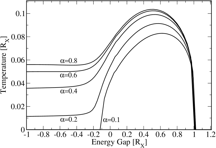
Figure 4: Phase boundaries for an EI as a function of $\alpha=m_{1}/m_{2}$. For $\alpha\ll 1$, the EI is strongly suppressed on the SM side because the finite temperature chemical potentials for CB electrons and VB holes are different for asymmetric band masses leading to breaking of Cooper-type electron-hole pairs. On the SC side, on the other hand, transition temperatures are only moderately reduced because of the $1/M$ dependence typical for BEC.

The SC-SM transition is driven by screening and Pauli blocking due to free charge carriers which, because of thermal excitation across a small energy gap, are not only available on the SM but also on the SC side. Neglecting on the SC side thermally excited charge carriers would lead to a much steeper phase boundary (dotted line in Fig. 3) and to a ${T_{c}}(0)\approx 0.45$, accidentally identical to the guess given for Sr in Ref. Jerome et al. (1967). The relative importance of phase space filling vs. screening can be estimated by comparing in Fig. 3 the SC-SM boundary (thick dashed line) with the hypothetical boundary (thin dashed line) arising when only screening is taken into account. In that case, the SC-SM boundary is given by $B=0$, which is equivalent to the ordinary Mott criterion $a_{X}\cdot q_{s}=1$ (see Eq. (34)). Contrasting the thin and thick dashed lines demonstrates that Pauli blocking cannot be ignored.

Phase boundaries for asymmetric band masses ($\alpha\neq 1$) are shown in Fig. 4. The differences of the condensation mechanisms on the SC and the SM side, respectively, can be most clearly seen in this figure, because the transition temperature of a BCS condensate of electron-hole pairs strongly depends on $\alpha$ whereas a BEC condensate of excitons does not. In contrast to equal band masses ($\alpha=1$), where the chemical potentials for the CB electrons and VB holes are pinned to $-\bar{E}_{g}/2$, as can be seen by inspection from Eqs. (22) and (24), asymmetric band masses lead to chemical potentials which are different for finite temperatures. Band asymmetry has thus a pair breaking effect on Cooper-type electron-hole pairs, similar to the effect a magnetic field has on Cooper pairs in superconductors. Accordingly, it leads to a strong suppression of ${T_{c}}({E_{g}})$ on the SM side. On the SC side, on the other hand, the EI is supported by tightly bound excitons and the 1/M dependence of the BEC transition temperature leads only to a moderate $\alpha$ dependence of ${T_{c}}({E_{g}})$. Thus, at $\alpha\neq 1$ the calculated phase boundary deviates substantially from the qualitative guess given in Fig. 1.

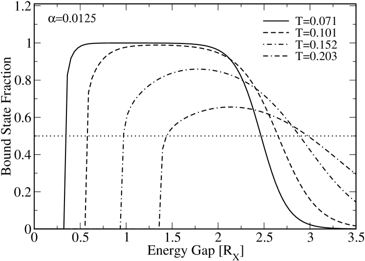
Figure 5: Bound state fraction of the exciton matter above an EI with $\alpha=0.0125$ as a function of the energy gap and for various temperatures. The interceptions with the dotted line indicate the energy gaps for which the bound state fraction is for the given temperature 50$\%$.

Our results seem to suggest that $\alpha\ll 1$ completely destroys the EI on the SM side even at ${T=0}$. This is however an artifact of our numerics which reaches here its limits of accuracy. The EI should be stable at $T=0$ (but not ${T}\neq 0$) for arbitrary mass ratios $\alpha$. Only anisotropies Zittartz (1967) and/or (multi-)valleys in the band dispersions separated by $2{\bf w}\neq{\bf K}$ with ${\bf K}$ a reciprocal lattice vector Halperin and Rice (1968) lead at $T=0$ to a suppression of the EI on the SM side for energy overlaps larger then a critical value. Note, multi-valleys in a band which are connected by a reciprocal lattice vector ${\bf K}$, i.e. identical multi-valleys, induce an “effective” mass asymmetry Zimmermann and thus the same pair breaking effect for finite temperatures as the real mass asymmetry considered above.

For $\alpha\ll 1$ the EI is almost entirely located on the SC side of the SC-SM boundary and within our approximations a BEC of excitons. Ignoring biexcitons, which, for strong mass asymmetry and attractive interactions, could interfere on the SC side with the EI Halperin and Rice (1968), two temperatures are required to characterize the EI and its exciton environment (halo of an EI): ${T_{M}}({E_{g}})$ where exciton formation sets in and ${T_{c}}({E_{g}})$ where condensation (phase coherence) is finally reached. Above ${T_{c}}({E_{g}})$ but below ${T_{M}}({E_{g}})$, a mixture of excitons, free electrons, and free holes exists, the composition of which depends on $T$ and ${E_{g}}$, as can be seen in Fig. 5, where we plot bound state fractions

$$\gamma=\frac{n_{1}^{b}}{n_{1}^{f}+n_{1}^{b}},$$ (41)

above ${T_{c}}({E_{g}})$ for an EI with $\alpha=0.0125$. Here, $n_{1}^{f}$ denotes the part of the total density corresponding to free electrons and $n_{1}^{b}$ the part bound in electron-hole pairs (excitons) as given by Eqs. (52) and (53), respectively.

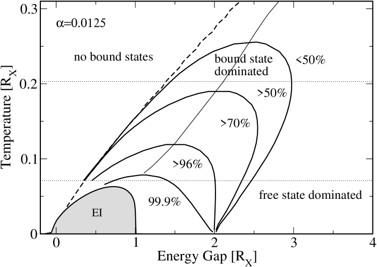
Figure 6: Phase boundary of an EI with $\alpha=0.0125$ and contours where the bound state fraction of its halo is 99.9$\%$, 96$\%$, 70$\%$, and 50$\%$, respectively. The temperature-dependent position of the maximum of the bound state fraction is shown by the thin solid line. Thin dashed lines indicate the temperatures for which in Fig. 7 the densities are plotted.

The bound state fraction indicates on which side of the chemical equilibrium $e+h\rightleftharpoons X$ the system is according to the mass-action law Zimmermann and Stolz (1985). Deep on the SC side, the chemical equilibrium is practically for all temperatures on the side of unbound electrons and holes and the bound state fraction is zero. Decreasing the energy gap leads to a shift of the chemical equilibrium to the exciton side signalled by an increasing bound state fraction which assumes a temperature dependent maximum (which can be very close to unity) before it abruptly decreases again to zero at and beyond the SC-SM transition. The depth and width of the maximum strongly depends on temperature. At low temperatures and large energy gaps the bound state fraction acquires a step-like shape (already visible by the solid line in Fig. 5). In that parameter range, the exponential tails of the Fermi and Bose functions contribute to Eqs. (52) and (53). Moreover, $\bar{B}\rightarrow B\rightarrow R_{X}$, $\bar{E}_{g}\rightarrow E_{g}$, and $\mu_{1}\approx\mu_{2}\approx-E_{g}/2$, leading to

$$\gamma\rightarrow 1-\frac{1}{1+(\frac{1+\alpha}{\alpha})^{\frac{3}{2}}\exp{[\beta(R_{X}-E_{g}/2)}]}.$$ (42)

Thus, as a consequence of the mass-action-law, the bound state fraction $\gamma$ has a step at $E_{g}=2\cdot R_{X}$ for $\beta E_{g},\beta(E_{g}-R_{X})\ll 1$.

The phase boundary for the EI with $\alpha=0.0125$ together with contours of the bound state fraction of its halo are displayed in Fig. 6. Almost the whole EI sits on the SC side, where it is surrounded by a large exciton rich region with bound state fractions significantly above 50$\%$. Remarkably, the bound state fraction approaches almost 100$\%$ before phase coherence is established. The exciton density in that region is not yet large enough for condensation to occur. Notice also, as a consequence of Eq. (42), all contours in Fig. 6 start at ${E_{g}}=2$ (exciton units).

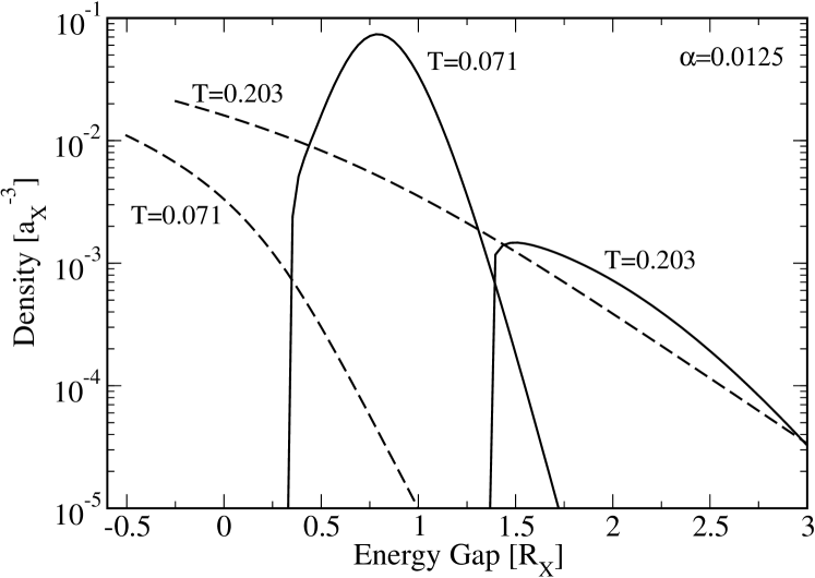
Figure 7: Bound (solid line) and free parts (dashed line) of the CB electron density as a function of the energy gap and for two temperatures above the EI (dotted lines in Fig. 6). Notice the very sharp decrease of the bound part of the density when the SC-SM transition is approached.

Figure 6 shows the exciton dominated part of the halo ($\gamma\geq 0.5$). In that region, we expect electrical resistivity anomalies similar to the ones observed in ${\rm TmSe_{0.45}Te_{0.55}}$ Neuenschwander and Wachter (1990); Bucher et al. (1991). Above ${T_{c}}({E_{g}})$ but below ${T_{M}}({E_{g}})$, for instance at $T=0.071$, diminishing ${E_{g}}$ (increasing pressure) pushes the system from the free state dominated to the bound state dominated regime. In the former, the resistivity is expected to decrease with decreasing ${E_{g}}$, because decreasing ${E_{g}}$ leads to an increase of free electrons and holes. The resistivity is here determined by the scattering of free charge carriers on imperfections and phonons. In the latter, however, decreasing ${E_{g}}$ leads not only to an increase of the free charge carriers but also to a rather strong increase of bound states, as can be seen in Fig. 7. Depending on temperature and $E_{g}$, the bound part of the density can be orders of magnitude higher then the density of the free charge carriers responsible for charge transport. As a result, an additional scattering channel is now available, free–bound state scattering, and strongly increases the resistivity. After a temperature dependent critical ${E_{g}}$, the bound part of the density decreases with decreasing energy gap. Hence, free–bound state scattering diminishes and the resistivity decreases again until it changes abruptly to a lower value at the SC-SM transition.

The results we presented in this section are for a generic Wannier-type EI. Contact with particular materials can be made by specifying the mass ratio $\alpha$, the exciton Rydberg $R_{X}$, and the exciton Bohr radius $a_{X}$ (or, alternatively, one of the two effective band masses $m_{i}$).

IV IV. Comparison with Experiment

We now discuss from the vantage point of our theory the experimental data for the pressure-induced SC-SM transition in ${\rm TmSe_{0.45}Te_{0.55}}$ Neuenschwander and Wachter (1990); Bucher et al. (1991); Wachter (2001); Wachter et al. (2004). Because of the fcc crystal structure Neuenschwander and Wachter (1990), the VB has a single maximum at the $\Gamma$ point while the CB has minima at the three $X$ points of the Brillouin zone. We can formally account for the three identical valleys of the CB as well as for the spin degeneracy by introducing on the rhs of Eqs. (20) and (21) multiplicity factors $g_{1}=6$ and $g_{2}=2$, respectively. The remaining equations are unchanged.

The mass ratio estimates for ${\rm TmSe_{0.45}Te_{0.55}}$ range from $\alpha=0.01$ to $\alpha=0.02$ Wachter et al. (2004) and optical measurements reveal an energy gap of 135 meV and an exciton binding energy of 75 meV Neuenschwander and Wachter (1990). The binding energy is thus rather large, which, in addition to the high exciton densities (see below), indicates that the effective-mass, Wannier-type model may not be quite adequate. Hybridization effects characteristic for a mixed-valence material such as ${\rm TmSe_{0.45}Te_{0.55}}$ may also not be completely captured by a two-band model. For our model to mimic the relevant parts of the band structure of ${\rm TmSe_{0.45}Te_{0.55}}$ we have to assume that during the excitonic instability, hybridization does not change much and the composition of the two bands is more or less fixed.

Although the multi-valley CB should favor a metallic electron-hole liquid Rice (1977), the experimentally observed increase of the resistivity cannot be explained by an emerging metallic phase. We consider therefore the static screening model, which a priori favors excitonic phases, as an effective model for ${\rm TmSe_{0.45}Te_{0.55}}$. The investigation of the competition between the two phases should be based on an improved description of screening (see the discussion following Eqs. (12)-(14)), taking however additional scattering processes into account, which most probably stabilize the EI in ${\rm TmSe_{0.45}Te_{0.55}}$ against an electron-hole liquid. Exciton-phonon scattering, for instance, could be such a process because the narrow VB in ${\rm TmSe_{0.45}Te_{0.55}}$ makes the exciton very susceptible to phonon dressing. Indeed, phonon signatures have been experimentally seen Wachter et al. (2004), but it is not clear whether they are the driving force for the excitonic instability or only triggered by it. In this respect it should be also mentioned that a static distortion associated with a density wave (which would be expected from the indirect gap) has not been found experimentally.

With these restrictions in mind, we present in Fig. 8 the phase boundary for $\alpha=0.015$, calculated with the multiplicity factors given above and scaled with the exciton Rydberg applicable to ${\rm TmSe_{0.45}Te_{0.55}}$, and compare it with the phase boundary for the “excitonic insulator” given by Wachter and coworkers in Ref. Bucher et al. (1991). Recall the phase boundary was constructed from the anomalous behavior of the electrical resistivity which, in a particular pressure and temperature range, first increases, peaks at a certain pressure, and then decreases with pressure until it terminates in a discontinuous jump. The on-set of the increase and the jump have been used to determine the entrance points for the “excitonic insulator” from the SC (open circles) and the SM from the “excitonic insulator” (open triangles), respectively. The ${E_{g}-T}$ values where the resistivity is maximal are given by the open squares. Fig. 8 also shows the data point (full diamond on the dotted line) where the linear increase of the thermal diffusivity has been observed. Wachter and coworkers claim that at this point ${\rm TmSe_{0.45}Te_{0.55}}$ is in a superfluid exciton state Wachter et al. (2004).

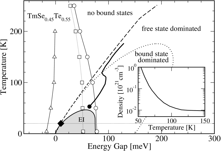
Figure 8: Comparison of the experimental data for ${\rm TmSe_{0.45}Te_{0.55}}$ Bucher et al. (1991); Wachter et al. (2004) with the phase boundary and the 50$\%$ contour calculated for an effective model applicable to this substance (see text for a description). Open circles, squares, and triangles denote the onset of the resistivity anomaly, the maximum of the resistivity, and the SC-SM transition, respectively Bucher et al. (1991). The full diamond on the dotted line indicates the point where the linear increase of the diffusivity has been found in Ref. Wachter et al. (2004). The inset shows the bound part of the density, $n_{1}^{b}$, along the thick solid line, which denotes the $(E_{g},T)$ points for which $n_{1}^{b}$ is maximal. At the full circle $n_{1}^{b}\approx 1.3\times 10^{21}~{}{\rm cm}^{-3}$.

Apparently, Wachter and coworkers Wachter et al. (2004) distinguish between an “excitonic insulator” at high temperatures and a superfluid exciton state at low temperatures which, however, is misleading, because the term “excitonic insulator” has been originally introduced to describe, on the SM side, a superfluid electron-hole condensate, similar to a superfluid condensate of Cooper pairs in a superconductor, and, on the SC side, an exciton condensate, similar to superfluid He 4 des Cloizeaux (1965); Keldysh and Kopaev (1964); Kozlov and Maksimov (1965); Jerome et al. (1967); Halperin and Rice (1968). Although the precise meaning of the terms “excitonic insulator” and “exciton condensation” changed in the course or their work and, in fact, was never fully in accordance with the original definitions, in more recent publications Wachter (2001); Wachter et al. (2004) they denote by the former an exciton liquid and by the latter a gas/liquid transition. The transition to the superfluid state they consider to be similar to the one in liquid He 4 Wachter et al. (2004).

Based on the results presented in the previous section, we suspect that the resistivity anomaly in ${\rm TmSe_{0.45}Te_{0.55}}$ is due to free–bound state scattering in the exciton rich part of the halo of an EI whereas the linear increase of the thermal diffusivity could signal an EI, understood as a macroscopic, phase coherent condensate of excitons. If our hypotheses are correct, we should be able to (i) relate the phase boundary of the “excitonic insulator” to the above 50$\%$ contours of the bound state fractions and (ii) find the experimental signature for superfluidity at a temperature where we would expect the EI.

The experimentally determined exciton Rydberg for ${\rm TmSe_{0.45}Te_{0.55}}$ puts the exciton rich part of the halo in the temperature range $T\sim$ 50 – 180 K, close to the temperature range where the resistivity anomaly and thus the “excitonic insulator” has been observed (open triangles, squares, and circles in Fig. 8). The bound part of the density in this range has also the correct order of magnitude. At $T=53~{}{\rm K}$ and ${E_{g}}=64~{}{\rm meV}$ (full circle in Fig. 8), for instance, we find, using $m_{1}=2.1m_{e}$ for the CB mass ($m_{e}$ bare electron mass), $n^{b}_{1}\approx 1.3\times 10^{21}~{}{\rm cm}^{-3}$ which compares favorably with the experimentally estimated exciton density of $3.9\times 10^{21}~{}{\rm cm}^{-3}$ Wachter (2001). The bound part of the density reaches its maximum along the thick solid line in Fig. 8. As can be seen in the inset, below 100 K, i.e. within the bound state dominated region, $n^{b}_{1}$ increases sharply. An improved theory, taking interactions between electron-hole pairs into account, could, when the repulsive part of the interaction dominates, display a gas/liquid transition in that temperature range. Hence, an exciton fluid, as proposed in Ref. Wachter et al. (2004), is conceivable below 100 K.

Below 50 K we find the EI, that is, the macroscopic, phase coherent condensate, very close to the 20 K (dotted line) where the linear increase of the diffusivity was observed at 13 kbar. From the associated isobar, we estimate the energy gap for that data point to be $\approx$ 20 meV (full diamond). Wachter and coworkers’ claim that this increase is due to the second sound of a superfluid is supported by our theory because the EI is entirely on the SC side. Hence, it constitutes a BEC of bosonic excitons, and not a BCS condensate of loosely bound electron-hole pairs, which may Kozlov and Maksimov (1966b) or may not display superfluidity Zittartz (1968). Without detailed knowledge of the interaction between electron-hole pairs, we cannot calculate superfluid properties. Nevertheless, the fact that the EI is on the BEC side makes it plausible that an improved theory would yield superfluidity, provided the interaction between excitons is dominantly repulsive.

The temperature dependence of the bound state fractions is consistent with values obtained form ab-initio numerical simulations of mass asymmetric electron-hole plasmas Fehske et al. (2005). The approximate T-matrix (28) on which the calculation of the bound state fractions is based captures therefore the essential physics. The interpretation of the experimental data is however hampered by two main difficulties.

First, the effective-mass model (1) and the resulting Wannier-type EI are, strictly speaking, not applicable to ${\rm TmSe_{0.45}Te_{0.55}}$. The exciton binding energy is too large compared to the energy gap. As a result, the bound state dominated region in Fig. 8 completely exhausts the maximal energy gap of 135 meV available at ambient pressure. Hence, the free state dominated region, where we expect a decrease of the resistivity with decreasing energy gap, occurs at energy gaps which cannot be realized.

Second, the bare energy gaps $E_{g}$, which we employ as a control parameter, are not necessarily the energy gaps given by Wachter and coworkers. Using the linear relation ${E_{g}(p,T=300~{}{\rm K})}={E_{g}(p=p_{a},T=300~{}{\rm K})}+{(dE_{g}/dp)(T=300~{}{\rm K})(p-p_{a})}$, with ${p_{a}}$ the ambient pressure, they convert (pressure, temperature) points, which they control experimentally, to (energy gap, temperature) points assuming the energy gap to be temperature independent and the closing rate to be temperature and pressure independent Neuenschwander and Wachter (1990); Bucher et al. (1991). At finite temperatures, however, bands are partially filled. The band gap renormalization to which the partial filling gives rise to leads not only to a strong temperature dependence of the energy gap but most probably also to a complicated pressure and temperature dependence of the closing rate. These effects were not incorporated in the assignment (pressure, temperature) $\leftrightarrow$ (energy gap, temperature) and perhaps the reason for the slight ‘left-turn’ of the experimental curves.

V V. Conclusions

We adopted a BEC-BCS crossover scenario to calculate the phase boundary of a pressure-induced EI using an isotropic, effective-mass model to describe the two bands involved in the excitonic instability and the dominant-term-approximation for the (statically screened) Coulomb interaction.

Assuming pressure to affect only the energy gap, we derived, within a meanfield approximation, a linearized gap equation for the anomalous selfenergy (order parameter) and determined, for a given energy gap ${E_{g}}$, the transition temperature ${T_{c}(E_{g})}$ as the highest temperature for which a non-trivial solution exists. The kernel of the gap equation depends on the chemical potentials for CB electrons and VB holes and on the screening wave number, all three have been determined self-consistently as a function of $T$ and ${E_{g}}$.

We pointed out that because pressure directly controls the chemical potentials, which moreover are constrained by charge neutrality, the meanfield theory is even for finite temperatures on par with T-matrix based crossover theories which include pair states in the equation for the chemical potential. We demonstrated by physical reasoning and calculation that in our case, pair states do not affect the chemical potentials as long as one stays within the framework of noninteracting pairs. As a result, the transition temperatures obtained from our meanfield theory coincide on the SC side with the transition temperatures for a BEC of non-interacting bosonic excitons. As a consistency check, we also determined ${T_{c}(E_{g})}$ on the SC side from the normal phase electron-hole T-matrix using the Thouless criterion.

Our main results are as follows: For equal band masses we found a very asymmetric phase boundary ${T_{c}(E_{g})}$, with a steeple on the SC side and a long tail on the SM side, directly reflecting the different character of the EI on the SC and SM side, respectively. Whereas on the SM side the EI comprises a BCS condensate of loosely bound Cooper pairs, the EI is a BEC of tightly bound excitons on the SC side. On the SM side, no simple exponential dependence of the transition temperature on the band overlap $|E_{g}|$ exists, as perhaps expected from the formal analogy to the BCS theory of superconductivity. We found mass asymmetry to strongly suppress pairing on the SM side because the different temperature dependencies of the chemical potentials for the CB electrons and VB holes have a pair-breaking effect on Cooper-type electron-hole pairs. The transition temperatures on the SC side, on the other hand, are only moderately modified, because the center-of-mass motion of excitons, which determines the transition temperatures on that side, depends only algebraically on the total mass (${T_{c}}\sim M^{-1}$). For very asymmetric band masses the EI is therefore rather fragile on the SM side and for finite temperatures almost entirely located on the SC side of the SC-SM transition. On the SC side, we also investigated the exciton density (more precisely, the part of the total density bound in excitons) in the region above $T_{c}$ which we called halo. Because of the mass-action-law, the exciton density strongly depends on temperature and energy gap. As a consequence, we expect pronounced resistivity anomalies in the halo due to free–bound state scattering.

Within the limitations of our model, we attempted an analysis of the experimental data for the pressure-induced SC-SM transition in ${\rm TmSe_{0.45}Te_{0.55}}$ Neuenschwander and Wachter (1990); Bucher et al. (1991); Wachter (2001); Wachter et al. (2004). From our theoretical point of view, the phase boundary, which was constructed from electrical resistivity data, traces most probably the exciton rich surroundings of an EI, where excitons dominate the total density, provide abundant scattering centers for the charge carriers, and induce the observed resistivity anomaly. Since we neglect interactions between excitons, we cannot decide whether a gas/liquid transition is also involved in the resistivity anomaly Wachter et al. (2004). The linear increase of the thermal diffusivity which was taken as a signal for superfluidity occurs at a temperature where we would expect the EI. Most importantly, however, the EI and the data point are on the SC side of the SC-SM transition, where the EI, that is, the macroscopic, phase coherent exciton state, consists of tightly bound bosonic excitons, which should support superfluidity when the repulsive core of the exciton-exciton interaction prevails over the attractive tail. Thus, the long journey of Wachter and coworkers Neuenschwander and Wachter (1990); Bucher et al. (1991); Wachter (2001); Wachter et al. (2004) may indeed have culminated Wachter et al. (2004) in the first observation of an exciton condensate.

We could not unambiguously proof the existence of a superfluid exciton condensate in ${\rm TmSe_{0.45}Te_{0.55}}$, most notably, because we did not allow the EI to compete with a metallic electron-hole liquid and because we did not account for the possibility of density waves. Although neither is supported by experimental data, both are in principle possible in a multi-valley band structure. Thus, to further substantiate the experimentalists claim from the theoretical side, a unified treatment of excitonic and electron-hole liquid phases, accounting also for the possibility of density waves, is clearly necessary, ideally for a model which avoids the effective-mass approximation, includes exciton-phonon scattering (which could stabilize excitonic phases against an electron-hole liquid), and an approximation scheme which takes the interaction between electron-hole pairs (or excitons) into account. The latter is important for the calculation of transport coefficients, which could be directly compared with experimental data, as well as for clarifying the role of biexciton formation, which, for large mass asymmetry, competes with the formation of the EI. Besides diagrammatic techniques Roepke (1994) and systematic mode-coupling approaches Cote and Griffin (1988, 1993), numerical simulation techniques Shumway and Ceperley (1999); Fehske et al. (2005) could proof very useful in this respect. In any case, the comparison between theory and experiment depends on the assignment (pressure, temperature) $\leftrightarrow$ (energy gap, temperature), which is rather subtle. To study the SC-SM transition along ‘iso-$E_{g}$’ instead of isobars would eliminate the uncertainties associated with this critical assignment and thus open the door for a more rigorous analysis of the excitonic phases in ${\rm TmSe_{0.45}Te_{0.55}}$.

*

Appendix A Appendix A: CB electron and VB hole densities in T-matrix approximation

In this appendix we determine the CB electron and VB hole densities as a function of the bare energy gap and the temperature. Thereby, we verify that even in the T-matrix approximation the chemical potentials for CB electrons and VB holes are, in leading order, not affected by exciton states.

Our starting point are the well-known formulae

$$n_{1} = \int\frac{d{\bf k}}{(2\pi)^{3}}\frac{d\omega}{2\pi}A_{11}({\bf k},\omega)n_{\rm F}(\omega),$$ (43)

$$\bar{n}_{2} = \int\frac{d{\bf k}}{(2\pi)^{3}}\frac{d\omega}{2\pi}A_{22}({\bf k},-\omega)n_{\rm F}(\omega)$$ (44)

for the CB electron and VB hole density, respectively. The spectral functions $A_{ii}$ are calculated with the selfenergies shown in Figs. (2a) and (2b). Expanding the spectral functions with respect to $\Gamma_{ii}=-2{\rm Im}\Sigma_{ii}$ leads to Zimmermann and Stolz (1985)

$$A_{ii}({\bf k},\omega) = 2\pi Z_{ii}({\bf k})\delta(\omega-\bar{e}_{i}({\bf k}))$$ (45)

$$+ \Gamma_{ii}({\bf k},\omega)\frac{\partial}{\partial\bar{e}_{i}({\bf k})}\frac{\rm P}{\omega-\bar{e}_{i}({\bf k})}$$

with the quasi-particle weight

$$Z_{ii}({\bf k}) = 1-\frac{\partial}{\partial\bar{e}_{i}({\bf k})}{\rm P}\int\frac{d\omega}{2\pi}\frac{\Gamma_{ii}({\bf k},\omega)}{\omega-\bar{e}_{i}({\bf k})}$$ (46)

and the renormalized single particle dispersion

$$\bar{e}_{i}({\bf k})={e}_{i}({\bf k})+\Sigma_{ii}^{X}({\bf k})+{\rm Re}\Sigma_{ii}^{L}({\bf k},\bar{e}_{i}({\bf k})+i\eta).$$ (47)

Let us first consider the CB electron density. Assuming the internal propagators in the selfenergy to describe free quasi-particles with a renormalized dispersion $\bar{e}_{i}$ but a quasi-particle weight unity, the selfenergy arising from the T-matrix reads

$$\Sigma_{11}^{L}({\bf k},\omega_{n}) = \int\frac{d{\bf q}}{(2\pi)^{3}}\frac{1}{\beta}\sum_{i\Omega_{n}}\Lambda_{12}({\bf k},{\bf k};{\bf q},i\Omega_{n}){\cal G}_{22}({\bf k}-{\bf q},i\omega_{n}-i\Omega_{n})$$ (48)

$$= \int\frac{d{\bf q}}{(2\pi)^{3}}\big{[}g(|{\bf k}-\frac{m_{1}}{M}{\bf q}|)\big{]}^{2}Z_{X}\frac{n_{\rm B}(E_{X}({\bf q}))+n_{\rm F}(\varepsilon_{2}({\bf k}-{\bf q})-\mu_{2})}{E_{X}({\bf q})-\varepsilon_{2}({\bf k}-{\bf q})+\mu_{2}-i\omega_{n}},$$

where we introduced the Bose function $n_{\rm B}$ and the exciton dispersion $E_{X}({\bf q})=\bar{E}_{g}-\bar{B}+q^{2}/2M$. To obtain Eq. (48), we approximated the renormalized dispersions $\bar{e}_{i}$, that is, the solutions of Eq. (47), by Eq. (16). For the electron-hole T-matrix we used Eq. (28) with Eq. (36) for the renormalized exciton propagator. Thus, after analytical continuation to real frequencies, we obtain

$$\Gamma_{11}({\bf k},\omega)=\int\frac{d{\bf q}}{(2\pi)^{2}}\big{[}g(|{\bf k}-\frac{m_{1}}{M}{\bf q}|)\big{]}^{2}Z_{X}\big{[}n_{\rm B}(E_{X}({\bf q}))+n_{\rm F}(\varepsilon_{2}({\bf k}-{\bf q})-\mu_{2})\big{]}\delta(E_{X}({\bf q})-\varepsilon_{2}({\bf k}-{\bf q})+\mu_{2}-\omega)$$ (49)

for the imaginary part of the selfenergy on the real frequency axis and, using a Kramers-Kronig relation,

$${\rm Re}\Sigma^{L}_{11}({\bf k},\omega)={\rm P}\int\frac{d\omega^{\prime}}{2\pi}\frac{\Gamma_{11}({\bf k},\omega^{\prime})}{\omega-\omega^{\prime}},$$ (50)

for the real part of the selfenergy on the real frequency axis.

If we now insert Eqs. (49) and (50) into Eq. (45), recall once again Eq. (16), and perform the ${\bf k}$-integration in Eq. (43), we find for the CB electron density

$$n_{1}=n_{1}^{f}+n_{1}^{b},$$ (51)

with a term arising from free electrons (in the sense defined above)

$$n_{1}^{f}=\int\frac{d{\bf k}}{(2\pi)^{3}}n_{\rm F}(\varepsilon_{1}({\bf k})-\mu_{1})$$ (52)

and a term

$$n_{1}^{b}=\int\frac{d{\bf p}d{\bf q}}{(2\pi)^{6}}\bigg{[}\frac{B+\frac{p^{2}}{2m}}{\bar{B}+\frac{p^{2}}{2m}}\bigg{]}^{2}\chi^{2}(p)Z_{X}F_{1}({\bf p},{\bf q})$$ (53)

due to the coupling of CB electrons and VB holes. The statistical factor is given by

$$F_{1}({\bf p},{\bf q}) = n_{\rm B}(E_{X}({\bf q}))\big{[}1-n_{\rm F}(\varepsilon_{1}({\bf p}+\frac{m_{1}}{M}{\bf q})-\mu_{1})$$ (54)

$$- n_{\rm F}(\varepsilon_{2}({\bf p}-\frac{m_{2}}{M}{\bf q})-\mu_{2})\big{]}$$

$$- n_{\rm F}(\varepsilon_{1}({\bf p}+\frac{m_{1}}{M}{\bf q})-\mu_{1})$$

$$\times n_{\rm F}(\varepsilon_{2}({\bf p}-\frac{m_{2}}{M}{\bf q})-\mu_{2}).$$

To derive Eq. (53) we transformed the ${\bf k}$-integration in Eq. (43) to an integration over the relative momentum ${\bf p}={\bf k}-(m_{1}/M){\bf q}$ when $\Gamma_{11}$ was part of the integrand and used definition (30) of the form factor.

In the limit $\beta E_{g}\ll 1$, Eq. (53) reduces to

$$n_{1}^{b}=\int\frac{d{\bf q}}{(2\pi)^{3}}n_{\rm B}(E_{X}({\bf q}))$$ (55)

because $F_{1}({\bf p},{\bf q})\rightarrow n_{\rm B}(E_{X}({\bf q}))$, $Z_{X}\rightarrow 1$, and the integration over ${\bf p}$ yields unity. The latter, a consequence of the optical theorem which the T-matrix has to obey, can be only ensured within a skeleton expansion.

The VB hole density can be calculated in a similar way. The result is

$$\bar{n}_{2}=\bar{n}_{2}^{f}+\bar{n}_{2}^{b}$$ (56)

with

$$\bar{n}_{2}^{f}=\int\frac{d{\bf k}}{(2\pi)^{3}}n_{\rm F}(\varepsilon_{2}({\bf k})-\mu_{2})$$ (57)

and a bound part $\bar{n}_{2}^{b}$ which is identical to $n_{1}^{b}$ given in Eq. (53). This is not unexpected, because for each CB electron participating in a bound state, a VB hole has to do so too.

As a consequence, the charge neutrality condition, $n_{1}=\bar{n}_{2}$, which fixes the chemical potentials for CB electrons and VB holes, reduces to $n^{f}_{1}=\bar{n}^{f}_{2}$. Neglecting the modifications of the single particle dispersions due to excitons, that is, ignoring interactions between excitons, which are higher order effects, the charge neutrality condition in the T-matrix approximation reduces to the meanfield charge neutrality condition.

With the chemical potentials determined from Eqs. (22) and (23), Eqs. (52) and (53) can be used to calculate, above the critical temperature ${T_{c}(E_{g})}$, the free and bound parts of the CB electron density and thus the bound state fraction (41).

Appendix B Appendix B: Separable approximation for the normal phase electron-hole T-matrix

Here we derive a separable approximation for the normal phase electron-hole T-matrix $\Lambda_{12}({\bf k,k^{\prime}};{\bf q},i\Omega_{n})$. In the vicinity of the exciton state the T-matrix factorizes with respect to ${\bf k}$ and ${\bf k^{\prime}}$. Thus, the separable approximation is a good approximation for energies not too far from the exciton energy. Since this energy range determines the physics of an EI, the separable approximation should be sufficient for our purpose.

The approximation is based on an expansion of the normal phase electron-hole T-matrix in terms of the eigenfunctions of an auxiliary Lippmann-Schwinger equation which takes into account screening due to spectator particles not participating in the bound state but ignores the spectators’ Pauli blocking. The phase space filling responsible for Pauli blocking is incorporated in a second step through a selfenergy for the exciton propagator. To avoid the numerical solution of the auxiliary Lippmann-Schwinger equation we approximate, as far as the calculation of the T-matrix is concerned, the screened Coulomb potential by the Hulthen potential. Eigenfunctions and binding energies are then analytically available.

The starting point is Eq. (26). In a first step, we break up the screened ladder equation into two equations. In an obvious notation

$$\Lambda_{12} = \Lambda_{12}^{(0)}+\Lambda_{12}^{(0)}[Q-Q^{(0)}]\Lambda_{12},$$ (58)

$$\Lambda_{12}^{(0)} = V_{s}+V_{s}Q^{(0)}\Lambda_{12}^{(0)}$$ (59)

with

$$Q^{(0)}({\bf k};{\bf q},i\Omega_{n})=\frac{1}{\bar{E}_{g}+\varepsilon_{1}({\bf k})+\varepsilon_{2}({\bf k}-{\bf q})-i\Omega_{n}}.$$ (60)

Note, this is an exact rewriting of Eq. (26), with the advantage that screening and Pauli blocking are now treated separately. Equation (59) introduces an auxiliary vertex which considers screening but not Pauli blocking. The full vertex is then obtained from Eq. (58).

Introducing relative momenta ${\bf p}$ according to ${\bf k}={\bf p}+(m_{1}/M){\bf q}$, Eq. (59) becomes

$$\Lambda_{12}^{(0)}({\bf p}+\frac{m_{1}}{M}{\bf q},{\bf p^{\prime}}+\frac{m_{1}}{M}{\bf q};{\bf q},i\Omega_{n})\!\! = \!\!V_{s}({\bf p}-{\bf p^{\prime}})$$ (61)

$$+ \!\!\int\frac{d{\bf p^{\prime\prime}}}{(2\pi)^{3}}\frac{V_{s}({\bf p}-{\bf p^{\prime\prime}})}{\bar{E}_{g}+\frac{q^{2}}{2M}+\frac{p^{\prime\prime 2}}{2m}-i\Omega_{n}}\Lambda_{12}^{(0)}({\bf p^{\prime\prime}}+\frac{m_{1}}{M}{\bf q},{\bf p^{\prime}}+\frac{m_{1}}{M}{\bf q};{\bf q},i\Omega_{n}),$$

which, with the identification

$$\Lambda_{12}^{(0)}({\bf p}+\frac{m_{1}}{M}{\bf q},{\bf p^{\prime}}+\frac{m_{1}}{M}{\bf q};{\bf q},i\Omega_{n})=T({\bf p},{\bf p^{\prime}};i\Omega_{n}-\bar{E}_{g}-\frac{q^{2}}{2M}),$$ (62)

reduces to

$$T({\bf p},{\bf p^{\prime}};i\Omega_{n})=V_{s}({\bf p}-{\bf p^{\prime}})+\int\frac{d{\bf p^{\prime\prime}}}{(2\pi)^{3}}\frac{V_{s}({\bf p}-{\bf p^{\prime\prime}})}{\frac{p^{\prime\prime 2}}{2m}-i\Omega_{n}}T({\bf p^{\prime\prime}},{\bf p^{\prime}};i\Omega_{n}).$$ (63)

Equation (63) is the T-matrix equation in the center-of-mass frame of an electron-hole pair interacting via a screened Coulomb potential. The medium occurs here only through the screening wave number $q_{s}$.

To solve Eq. (63) we employ the unitary pole expansion for $T({\bf p},{\bf p^{\prime}};i\Omega_{n})$, using eigenfunctions of the corresponding Lippmann-Schwinger equation at fixed energy as a basis Harms (1970). In particular, we take the eigenfunctions at energy $i\Omega_{n}\rightarrow-B$, with $-B$ the energy of the lowest bound state. Truncating the expansion after the first term yields (for an isotropic system)

$$T(p,p^{\prime};i\Omega_{n})=g(p)\cdot d_{X}(i\Omega_{n})\cdot g(p^{\prime})$$ (64)

with

$$d_{X}(z)=\frac{-1}{z+B},$$ (65)

which can be interpreted as a screened exciton propagator, and form factors defined in Eq. (30). For the Hulthen potential the screened exciton wavefunction $\chi(p)$, and thus the from factor $g(p)$, as well as the screened binding energy $B$ can be obtained analytically and are given by Eqs. (33) and (34), respectively.

Combining now Eq. (64) with Eq. (62) leads to

$$\Lambda_{12}^{(0)}({\bf p}+\frac{m_{1}}{M}{\bf q},{\bf p^{\prime}}+\frac{m_{1}}{M}{\bf q};{\bf q},i\Omega_{n})=g(p)\cdot d_{X}(i\Omega_{n}-\bar{E}_{g}-\frac{q^{2}}{2M})\cdot g(p^{\prime})$$ (66)

for the auxiliary vertex. To obtain the full vertex, we write $\Lambda_{12}$ in a similar form,

$$\Lambda_{12}({\bf p}+\frac{m_{1}}{M}{\bf q},{\bf p^{\prime}}+\frac{m_{1}}{M}{\bf q};{\bf q},i\Omega_{n})=g(p)\cdot D_{X}({\bf q},i\Omega_{n}-\bar{E}_{g}-\frac{q^{2}}{2M})\cdot g(p^{\prime}),$$ (67)

but with a renormalized exciton propagator $D_{X}({\bf q},i\Omega_{n})$ instead of the screened exciton propagator $d_{X}(i\Omega_{n})$. Inserting Eqs. (66) and (67) into Eq. (58), leads to a Dyson equation,

$$D_{X}({\bf q},i\Omega_{n})=d_{X}(i\Omega_{n})+d_{X}(i\Omega_{n})M_{X}({\bf q},i\Omega_{n})D_{X}({\bf q},i\Omega_{n}),$$ (68)

for the renormalized exciton propagator $D_{X}({\bf q},i\Omega_{n})$ with the selfenergy $M_{X}({\bf q},i\Omega_{n})$ given in Eq. (31). The selfenergy takes Pauli blocking into account. Switching in Eq. (67) from the relative momenta ${\bf p}$ and ${\bf p^{\prime}}$ back to the original momenta ${\bf k}$ and ${\bf k^{\prime}}$, we recover Eq. (28) for the full vertex.