Solitons in coupled atomic-molecular Bose-Einstein condensates

Abstract

We consider coupled atomic-molecular Bose-Einstein condensate system in a quasi-one-dimensional trap. In the vicinity of a Feshbach resonance the system can reveal parametric soliton-like behavior. We analyze bright soliton, soliton train and dark soliton solutions for the system in the trap and in the presence of the interactions between particles and find the range of the system parameters where the soliton states can be experimentally prepared and detected.

I Introduction

The experimental success in realizing a Bose-Einstein condensate (BEC) in dilute atomic gases bec_rb87 ; bec_na23 ; bec_li7 has led to the strong experimental and theoretical activity in this field. Dilute gases turn out to be an ideal system for realizing and high accuracy manipulation of various quantum many-body phenomena. The nonlinear nature of a BEC in the mean field description allows investigations of e.g. vortex lattices vl_1st_obs ; ketterle ; vort_latt_str , four-wave mixing fw_mix_exp ; fw_mix_theory , Josephson-like oscillations jos_theory ; jos_exp and solitons in the system. The latter have been realized experimentally for a quasi one-dimensional (1D) atomic BEC with repulsive effective interactions (so-called dark solitons) burg ; phil and with attractive interactions (bright solitons) sal ; trains_li . There are also proposals to prepare experimentally solitons in a mixture of bosonic and fermionic atoms trainsBF and in an atomic BEC with a time-dependent scattering length Kevrekidis ; abdullaev ; pelinovsky ; sol_time_scatt ; trippenbach .

In the present publication we consider another type of solitonic solutions. That is, parametric solitons, which in the context of nonlinear optics occur as a result of a coupling between fields in a nonlinear medium such that each field propagates as solitons kivshar . In the coupled atomic-molecular BEC, there is a nonlinear resonant transfer between atoms and molecules, as well as terms proportional to the densities. The solitons of this type have been investigated in nonlinear optics karpierz95 ; drummond96 ; berge and in the problem of the self-localization of impurity atoms in a BEC st06 . In the context of the atomic-molecular BECs the parametric solitons have been analyzed in Ref. drummondPRL98 ; drummondPRA04 . The latter publications consider, in principle, solitons in free space in any dimension but they concentrate on the existence and stability of the soliton like states in 3D free space. However, a profound analysis of the system in a quasi 1D trap is missing and methods for experimental preparation and detection are not considered. Trapping an atomic BEC in a quasi 1D potential allowed realizing remarkable experiments where bright soliton wave packets travelled in 1D space (still with transverse confinement) without spreading sal ; trains_li . In the case of the coupled atomic-molecular BECs, experimentalists have to face a problem of atomic losses, which becomes significant at a Feshbach resonance. We show that to overcome this obstacle one has to deal with moderate particle densities, and consider the range of the system parameters where preparation and detection of the solitons are sufficiently fast to be able to compete with the loss phenomenon. Moreover, the soliton states can be prepared at the magnetic field slightly off the resonance value, where the number of created molecules is still considerable but the rate of atomic losses much smaller than at the resonance.

The paper is organized as follows. In Sec. II we introduce the model of the system and in Sec. III we analyze different solitonic states. Section IV is devoted to analysis of methods for experimental preparation and detection.

II The Model

In order to obtain a complete model of a Feshbach resonance in an atomic BEC, the intermediate bound states (molecules) have to be included explicitly in the Hamiltonian. At the resonance, the number of molecules becomes considerable and a second (molecular) BEC is formed. We take into account two body atom-atom, molecule-molecule and atom-molecule collisions, as well as the term responsible for the creation of molecules, i.e. transfer of pairs of atoms into molecules and vice versa timm :

$$\hat{H} = \large{\int}{\rm d}^{3}r\Big{(}\hat{\psi}^{\dagger}_{a}\Big{[}-\frac{\hbar^{2}}{2m}\nabla^{2}+U_{a}(\vec{r})+\frac{\lambda_{a}}{2}\hat{\psi}^{\dagger}_{a}\hat{\psi}_{a}\Big{]}\hat{\psi}_{a}$$ (1)

$$+ \hat{\psi}^{\dagger}_{m}\Big{[}-\frac{\hbar^{2}}{4m}\nabla^{2}+U_{m}(\vec{r})+{\cal E}+\frac{\lambda_{m}}{2}\hat{\psi}^{\dagger}_{m}\hat{\psi}_{m}\Big{]}\hat{\psi}_{m}$$

$$+ \lambda_{am}\hat{\psi}^{\dagger}_{a}\hat{\psi}_{a}\hat{\psi}^{\dagger}_{m}\hat{\psi}_{m}+\frac{\alpha}{\sqrt{2}}\big{[}\hat{\psi}^{\dagger}_{m}\hat{\psi}_{a}\hat{\psi}_{a}+\hat{\psi}_{m}\hat{\psi}^{\dagger}_{a}\hat{\psi}^{\dagger}_{a}\big{]}\Big{)},$$ (2)

where $m$ is the atomic mass, $\lambda_{a}$, $\lambda_{m}$, $\lambda_{am}$ are coupling constants for the respective interactions, and $\alpha$ determines the strength of the resonance. The $\cal E$ parameter is a difference between the bound state energy of two atoms and the energy of a free atom pair timm , and it can be varied by means of a magnetic field. $U_{a}(\vec{r})$ and $U_{m}(\vec{r})$ stand for atomic and molecular trapping potentials, respectively. We would like to point out that in our model an internal structure of molecules and all processes involving the internal structure are neglected and we consider only a single molecular state described by the operator $\hat{\psi}_{m}$.

In the present paper we consider the system parameters mainly related to ⁸⁷Rb atoms. That is, the mass $m$, the coupling constant $\lambda_{a}$ and the strength of the resonance $\alpha$ correspond to ⁸⁷Rb atoms and the Feshbach resonance that occurs at the magnetic field of $B_{\rm r}=685.43$ G durrprec . However, because the precise values of the coupling constants $\lambda_{m}$ and $\lambda_{am}$ are unknown these constants have to be chosen arbitrary. For simplicity we assume $\lambda_{am}\approx\lambda_{m}\approx\lambda_{a}=4\pi\hbar^{2}a/m$, where $a=5.7$ nm is the value of the atomic scattering length far from a Feshbach resonance. In Sec. III we show that this assumption is not essential because in a broad range of $\lambda_{m}$ and $\lambda_{am}$ values there exist stable soliton solutions. The resonance strength parameter $\alpha$ can be expressed in terms of $\Delta B$, the resonance width, and $\Delta\tilde{\mu}$, difference between magnetic moments of a molecule and a free atom pair, $\alpha=\sqrt{4\pi\hbar^{2}a\Delta\tilde{\mu}\Delta B/m}$. We have chosen for investigation the broad resonance which occurs at the magnetic field $B_{\rm r}=685.43$ G where $\Delta B=0.017$ G and $\Delta\tilde{\mu}=1.4\mu_{B}$ ($\mu_{B}$ is the Bohr magneton) durrprec . We focus on the case where the system is prepared in a harmonic trap with so strong radial confinement that the radial frequency of the trap exceeds the chemical potential of the system. Then, only the ground states of the transverse degrees of freedom are relevant and the system becomes effectively 1D. The chosen trap frequencies are $\omega_{m,\perp}=\omega_{a,\perp}=2\pi\times 1500$ Hz and $\omega_{m,x}=\omega_{a,x}=2\pi\times 10$ Hz . The effective 1D coupling constants are obtained by assuming that atoms and molecules are in the ground states of the 2D harmonic trap of frequencies $\omega_{m,\perp}$ and $\omega_{a,\perp}$, and by integrating the energy density over transverse variables. In the harmonic oscillator units,

$$E_{0} = \hbar\omega_{a,x},$$ (3)

$$x_{0} = \sqrt{\frac{\hbar}{m\omega_{a,x}}},$$ (4)

$$\tau_{0} = \frac{1}{\omega_{a,x}},$$ (5)

where $E_{0}$, $x_{0}$ and $\tau_{0}$ are energy, length and time units, respectively, one obtains

$$\lambda_{a}=\lambda_{m}=\lambda_{am}\approx 0.505,$$ (6)

and

$$\alpha\approx 41.0.$$ (7)

The equations of motion for the atomic and molecular mean fields, corresponding to the Hamiltonian (2), in the 1D model, in the units (5), are

$$i\frac{\partial\phi_{a}}{\partial t} = \Big{[}-\frac{1}{2}\frac{\partial^{2}}{\partial x^{2}}+\frac{1}{2}x^{2}+\lambda_{a}N|\phi_{a}|^{2}+\lambda_{am}N|\phi_{m}|^{2}\Big{]}\phi_{a}$$ (8)

$$+ \alpha\sqrt{2N}\phi_{m}\phi^{*}_{a}$$

$$i\frac{\partial\phi_{m}}{\partial t} = \Big{[}-\frac{1}{4}\frac{\partial^{2}}{\partial x^{2}}+x^{2}+\varepsilon+\lambda_{m}N|\phi_{m}|^{2}+\lambda_{am}N|\phi_{a}|^{2}\Big{]}\phi_{m}$$ (9)

$$+ \alpha\sqrt{\frac{N}{2}}\phi^{2}_{a},$$

where $N$ is the total number of atoms in the system timm . The 1D detuning $\varepsilon$ is modified with respect to the corresponding $\cal E$ in the 3D case, i.e. $\varepsilon={\cal E}+(\omega_{a,\perp}-2\omega_{m,\perp})/\omega_{a,x}={\cal E}-150$. The wave-functions $\phi_{a}(x)$ and $\phi_{m}(x)$ are normalized so that

$$\int{\rm d}x\left(|\phi_{a}(x)|^{2}+2|\phi_{m}(x)|^{2}\right)=1.$$ (10)

The Eqs. (9) look like a pair of coupled Gross-Pitaevskii equations but with an extra term responsible for the transfer of atoms into molecules and molecules into atoms. The presence of this term allows for solutions that reveal parametric soliton like behavior.

The mean field model (9) can be used if the condensates are nearly perfect. That is, if the depletion effects are negligible which is usually true even for small particle number in a system dziarmaga . The model neglects also effects of particle losses. The latter can be described by introducing terms proportional to densities with imaginary coefficients (that can be estimated provided there is precise experimental analysis of the losses in the vicinity of the Feshbach resonance) in the square brackets of Eqs. (9) yurovsky03 ; yurovsky04 .

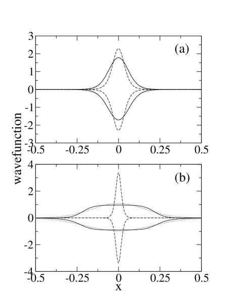
Figure 1: Solid lines correspond to the ground state solutions of Eqs. (12) for $N=100$ (a) and $1000$ (b). Dashed lines are the analytic solutions (16) corresponding to the case without the interaction between particles and in the absence of the trapping potentials. Dotted lines are related to the gaussian ansatz (21) – for $N=100$ the states are almost the same as the exact ones. The atomic wavefunctions $\phi_{a}>0$, whereas the molecular ones $\phi_{m}<0$. The ground states of Eqs. (12) correspond to the detuning chosen so that $\langle\phi_{a}|\phi_{a}\rangle=\langle\phi_{m}|\phi_{m}\rangle$, i.e. $\varepsilon=-900.53$ (a) and $\varepsilon=-1505.25$ (b). Note that the widths of the states are much smaller than the width of the ground state of the harmonic oscillator, which indicates that even for a very small particle number the nonlinearities in Eqs. (12) determine the shapes of the states.

III Soliton like solutions

III.1 Bright soliton solutions

The time-independent version of Eqs. (9) reads

$$\mu\phi_{a} = \Big{[}-\frac{1}{2}\frac{\partial^{2}}{\partial x^{2}}+\frac{1}{2}x^{2}+\lambda_{a}N\phi_{a}^{2}+\lambda_{am}N\phi_{m}^{2}\Big{]}\phi_{a}$$ (11)

$$+ \alpha\sqrt{2N}\phi_{m}\phi_{a}$$

$$2\mu\phi_{m} = \Big{[}-\frac{1}{4}\frac{\partial^{2}}{\partial x^{2}}+x^{2}+\varepsilon+\lambda_{m}N\phi_{m}^{2}+\lambda_{am}N\phi_{a}^{2}\Big{]}\phi_{m}$$ (12)

$$+ \alpha\sqrt{\frac{N}{2}}\phi^{2}_{a},$$

where $\mu$ is the chemical potential of the system, and we have assumed that the solutions are chosen to be real. The ground state of the system described by Eqs. (12) can be found numerically. However, in the absence of the trapping potentials and for $\lambda_{a}=\lambda_{m}=\lambda_{am}=0$, there exists an analytical solution karpierz95 ; drummond96 ; berge if

$$\varepsilon=-\frac{6}{l^{2}},$$ (13)

where

$$l=\Big{(}\frac{18}{\alpha^{2}N}\Big{)}^{1/3}.$$ (14)

That is,

$$\phi_{a}(x) = \pm\frac{a}{\cosh^{2}\left({\frac{x}{l}}\right)},$$ (15)

$$\phi_{m}(x) = -\frac{a}{\cosh^{2}\left({\frac{x}{l}}\right)},$$ (16)

where

$$a = \frac{3}{\sqrt{2N}\alpha l^{2}},$$ (17)

$$\mu = -\frac{2}{l^{2}},$$ (18)

describe the parametric bright soliton of width $l$, which can propagate in time without changing its shape. The corresponding time-dependent solution is

$$\phi_{a}(x,t) = \pm\frac{a{e^{ivx}}{e^{-i({v}^{2}+\mu)t}}}{\cosh^{2}\left({\frac{x-vt}{l}}\right)}$$ (19)

$$\phi_{m}(x,t) = -\frac{a{e^{2ivx}}{e^{-2i({v}^{2}+\mu)t}}}{\cosh^{2}\left({\frac{x-vt}{l}}\right)},$$ (20)

where $v$ is the propagation velocity. The analytical solution is known for a particular value of the detuning $\varepsilon$ but solutions revealing soliton like character exist also for other values. By changing $\varepsilon$ we can obtain solitons but with unequal population of atomic and molecular condensates.

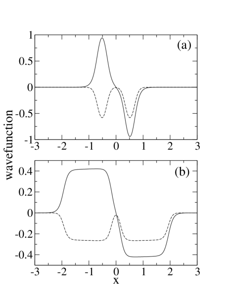
Figure 2: Two bright soliton solution for $N=100$ (a) and $N=1000$ (b). The atomic wave-functions $\phi_{a}(x)$ are odd functions while the molecular wave-functions $\phi_{m}(x)$ are the even ones. Note that populations of atomic and molecular condensates are unequal for the value of the detuning chosen, i.e. $\varepsilon=0$. Note that the widths of the states in panel (a) are much smaller than the width of the first excited state of the harmonic oscillator, which indicates that even for a very small particle number the nonlinearities in Eqs. (12) determine the shapes of the states.

In the presence of the (repulsive) interactions, the solutions for the ground states reveal wave-packets that, for increasing total number of atoms $N$ in the system, become wider and wider. Indeed, for $\lambda_{a}>0$, $\lambda_{m}>0$ and $\lambda_{am}>0$ and with increasing $N$, the repulsive interactions are stronger (see Fig. 1). Unlike the repulsive nature of the interactions, the term responsible for the transfer between atoms and molecules acts as an attractive potential. For $N$ not too high, the transfer term dominates over the interaction terms and it alone determines the shape of the wave-packets. In Fig. 1 we can see that the ground state solution for $N=100$ is only slightly wider than the analytical solution (16). In Fig. 1 we also present the results of variational analysis of Ref. drummondPRA04 (including also nonzero coupling constants $\lambda_{m}$ and $\lambda_{am}$) where the solutions have been assumed to be given by gaussian functions,

$$\phi_{a}(x)=\tilde{A}e^{-\tilde{a}x^{2}}, \phi_{b}(x)=\tilde{B}e^{-\tilde{b}x^{2}}.$$ (21)

Requiring the same fraction of atoms and molecules, for $N=100$ ($N=1000$), we obtain $\tilde{A}=1.77$, $\tilde{a}=139.54$, $\tilde{B}=1.70$, $\tilde{b}=117.43$, $\varepsilon=-900$ ($\tilde{A}=1.08$, $\tilde{a}=19.58$, $\tilde{B}=0.97$, $\tilde{b}=12.47$, $\varepsilon=-1429$) which fits quite well to the exact solutions.

Even in the presence of the interactions the obtained solutions do not loose their solitonic character, which can be verified by the time evolution of the states in 1D free space (i.e. in the presence of the transverse confinement but with the axial trap turned off) — see Sec. IV for examples of the time evolution. The existence of the solitons can be also verified employing the Gaussian ansatz (21). Indeed, in the absence of the axial traps we have checked that, for $N=1000$, $\lambda_{m}\in(0,2\lambda_{a})$ and $\lambda_{am}\in(-2\lambda_{a},2\lambda_{a})$, the solutions exist with $\tilde{a}$ and $\tilde{b}$ in the range (1,20000) lam . It shows also that the choice of equal coupling constants is not essential in order to deal with soliton like solutions.

All stationary states of the Gross-Pitaevskii equations (12) have been obtained numerically by means of the so-called imaginary time evolution which implies they are stable solutions of these non-linear coupled Schrödinger equations.

III.2 Two bright soliton and dark soliton solutions

In the absence of the trapping potential and for $\lambda_{a}=\lambda_{m}=\lambda_{am}=0$ one can find an asymptotic solution of Eqs. (12) that reveals two bright soliton structure,

$$\phi_{a}(x) = \frac{a}{\cosh^{2}\left({\frac{x-q}{l}}\right)}\pm\frac{a}{\cosh^{2}\left({\frac{x+q}{l}}\right)}$$ (22)

$$\phi_{m}(x) = -\frac{a}{\cosh^{2}\left({\frac{x-q}{l}}\right)}-\frac{a}{\cosh^{2}\left({\frac{x+q}{l}}\right)},$$ (23)

valid for $q\gg l$, where

$$a = \frac{3}{\sqrt{2N}\alpha l^{2}},$$ (24)

$$\mu = -\frac{2}{l^{2}},$$ (25)

$$l = \Big{(}\frac{36}{\alpha^{2}N}\Big{)}^{1/3}$$ (26)

$$\varepsilon = -\frac{6}{l^{2}}.$$ (27)

In the presence of the traps and the interactions we may look for similar solutions. Analysis of Eqs. (12) shows that due to the fact that the trapping potentials are even functions we may expect that eigenstate functions are either even or odd. However, because of the presence of the $\phi_{a}^{2}$ term in the second of Eqs. (12), an even function is the only possibility for $\phi_{m}$. In Fig. 2 there are examples of the two bright soliton solutions for $N=100$ and $N=1000$.

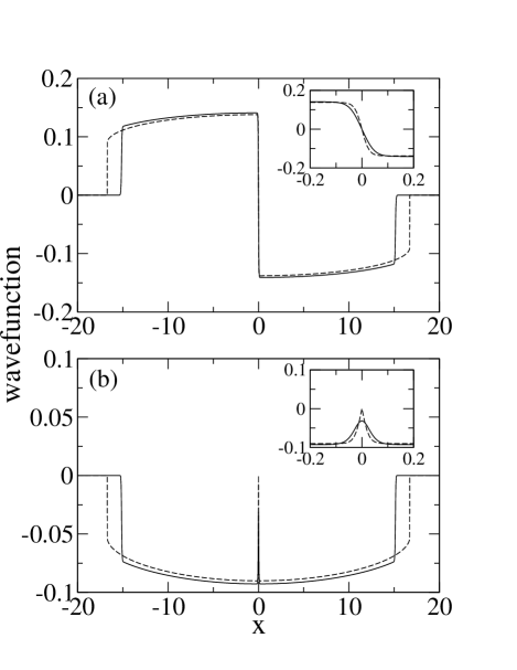
Figure 3: The soliton solution (solid lines), obtained for the detuning $\varepsilon=0$, compared to the solution within the Thomas-Fermi approximation (dashed lines). Panel (a) shows the atomic wavefunctions while panel (b) the molecular ones. The insets show the same as the main panels but with plots enlarged around the trap center.

With an increasing number of particles the shapes of the density profiles change. For large particle numbers the healing length of the system becomes much smaller than the size of the system and one obtains density shapes that resemble the dark soliton state known for the Gross-Pitaevskii equation in the case of repulsive interparticle interactions burg ; phil — the results for $N=10^{5}$ are shown in Fig. 3. Here, however, only the atomic wave-function $\phi_{a}(x)$ exhibits a phase flip. We can approximate the exact eigenstates by (see Fig. 3)

$$\phi_{a}(x) \approx \phi^{\rm TF}_{a}(x)\tanh\left(\frac{x}{\xi}\right),$$ (28)

$$\phi_{m}(x) \approx \phi^{\rm TF}_{m}(x)\left|\tanh\left(\frac{x}{\xi}\right)\right|,$$ (29)

where

$$\xi=\frac{1}{\sqrt{\lambda_{a}N\left(|\phi_{a}|^{2}+|\phi_{m}|^{2}\right)}},$$ (30)

and

$$\phi^{\rm TF}_{m}(x) = \frac{\gamma}{2}-\sqrt{\frac{\gamma^{2}}{4}+\frac{2\mu-x^{2}}{6\lambda_{a}N}},$$ (31)

$$\phi^{\rm TF}_{a}(x) = \sqrt{\frac{2\mu-x^{2}}{2\lambda_{a}N}-\frac{\sqrt{2}\alpha}{\lambda_{a}\sqrt{N}}\phi^{\rm TF}_{m}(x)-\left[\phi^{\rm TF}_{m}(x)\right]^{2}},$$ (32)

$$\gamma = \frac{\sqrt{2}}{3\alpha\sqrt{N}}\left(\frac{x^{2}-2\mu}{2}-\frac{\alpha^{2}}{\lambda_{a}}\right),$$ (33)

are solutions for the ground state of the mean field equations within the Thomas-Fermi approximation, and the chemical potential $\mu$ can be found from the normalization condition (10).

Finally we would like to mention that in the case of the harmonic trap, having any solutions $\phi_{a0}(x)$ and $\phi_{m0}(x)$ of the time-independent problem, Eqs. (12), corresponding to the chemical potential $\mu$, one can easily obtain time evolution of the initial wave-functions $\phi_{a0}(x-q)$ and $\phi_{m0}(x-q)$, i.e.

$$\phi_{a}(x,t) = \phi_{a0}(x-q)e^{-i\mu t}e^{i[\dot{q}x-S(q)]},$$ (34)

$$\phi_{m}(x,t) = \phi_{m0}(x-q)e^{-i2\mu t}e^{2i[\dot{q}x-S(q)]},$$ (35)

where

$$S(q)=\frac{1}{2}\int_{t_{0}}^{t}{\rm d}t^{\prime}\left[\dot{q}^{2}(t^{\prime})-q^{2}(t^{\prime})\right],$$ (36)

and

$$\frac{{\rm d}^{2}q}{{\rm d}t^{2}}+q=0.$$ (37)

The proof can be done by direct substitution of (35) into (9). This indicates that, similarly as in the case of the Gross-Pitaevskii equation for a single condensate in a harmonic trap, time evolution of the translated stationary solutions reveals harmonic oscillations of the center of mass of the particle cloud.

IV Experimental creation and detection

To create experimentally a bright soliton state we propose to start with a purely atomic condensate in a quasi-1D trap with the magnetic field significantly higher than the resonance value. Then the field should be slowly decreased until it reaches the resonance. Actually, from the experimental point of view, it is better to end up slightly off the resonance because the rate of atomic losses is then much smaller than the rate at the resonance. The final populations of atomic and molecular condensates are unequal in such case but they still reveal solitonic character. In the following we analyze different velocities of the sweeping of the field in order to find the optimal shape of the state.

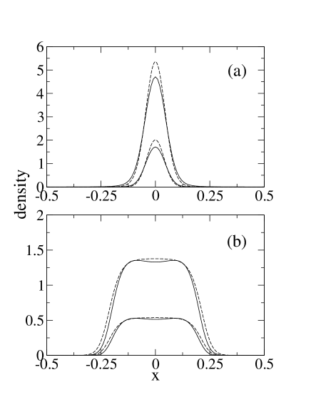
Figure 4: Solid lines: density profiles of solitons excited after the magnetic field sweeping for $N=100$ (a) and $N=1000$ (b). The sweeping lasted $95.5$ ms (a) and $93.8$ ms (b). Dashed lines show the exact ground states corresponding to the magnetic field at the end of the sweeping. The detuning $\varepsilon=0$ at the end of the evolution. Top curves, in each panel, are related to densities of atoms and bottom ones to densities of molecules.

We have done numerical calculations for $N$ in the range between 100 and 10000. Assuming that the initial state is an almost purely atomic BEC, i.e. the ground state of the system far from the resonance, the detuning $\varepsilon$ has been varied linearly in time from 3331 to 0 ($\Delta\varepsilon=3331$ corresponds to $\Delta B=0.017$ G). In order to obtain a nice solitonic state, the evolution time has to be carefully chosen. We have found that the square overlap between a final state and a desired eigenstate oscillates as a function of the evolution time. Therefore one has to find a proper value of the evolution time, corresponding to a maximum value of the square overlap. From the experimental point of view, the shorter the evolution time the better because that allows one to reduce particle losses significant close to the resonance. In Fig. 4 there are results for $N=100$ and $N=1000$ corresponding to the optimized evolution time and compared with the ground states at the resonance. One can see that despite quite short evolution times ($95.5$ ms and $93.9$ ms for $N=100$ and $N=1000$, respectively), the final states reproduce the exact ground states quite well, i.e. the square overlaps are $0.94$ and $0.92$. For $N=10000$ the shortest evolution time that results in a reasonably high squared overlap (i.e. $0.83$) is $90.7$ ms. Note that the population of the molecular BEC is smaller than the population of the atomic BEC because the final value of the detuning corresponds to the magnetic field slightly off the resonance.

Using the procedure described above it is possible not only to create a single bright soliton but also excite states that reveal multi-peak structure (so-called “soliton trains” trains_li ). Actually, deviations from the optimal sweeping time of the magnetic field result in multi-peak structure of the atomic and molecular densities. An example of $N=1000$, where the soliton train is particularly well reproduced, is shown in the Fig. 5. The calculations have been performed starting with the same initial state and the magnetic field value as in Fig. 4, but the sweeping time is now $25.5$ ms.

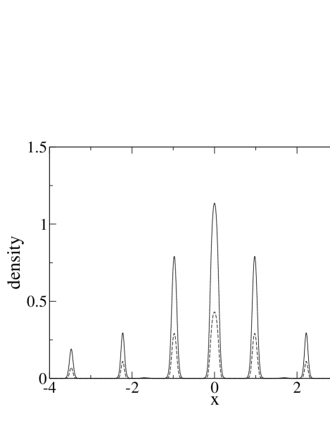
Figure 5: Soliton train obtained for $N=1000$ after the sweeping of the magnetic field that lasted $25.5$ ms. Solid line indicates the atomic density while the dashed line the molecular density.

Figure 6: Time evolution of a soliton state for $N=1000$ in an inhomogeneous magnetic field ($B_{\rm grad}=1$ G/cm), for the detuning (41) $\varepsilon_{\rm grad}=0$. Panel (a) shows the atomic wave-packet, panel (b) the molecular one. The time $t=1$ in the units (5) corresponds to $15.9$ ms.

Figure 7: Time evolution of a soliton state for $N=100$ in an inhomogeneous magnetic field ($B_{\rm grad}=1$ G/cm), for the detuning (41) $\varepsilon_{\rm grad}=2216$. Panel (a) shows the atomic wave-packet, panel (b) the molecular one. The time $t=1$ in the units (5) corresponds to $15.9$ ms.

Figure 8: Time evolution of a soliton state for $N=1000$ (b) in an inhomogeneous magnetic field ($B_{\rm grad}=1$ G/cm), for the detuning (41) $\varepsilon_{\rm grad}=2216$. Panel (a) shows the atomic wave-packet, panel (b) the molecular one. The time $t=1$ in the units (5) corresponds to $15.9$ ms.

In Ref. sal ; trains_li detection of time evolution of wave-packets without spreading in the presence of the transverse confinement but with the axial trap turned off (or even in the presence of an inverted axial potential) was an experimental signature of the bright soliton excitation in an atomic BEC with attractive atom-atom interaction. In the present case we can use the same test to check if the states obtained reveal stable soliton like character. It turns out that indeed all the states presented do not spread when the axial trap is turned off during time evolution lasting even $100$ ms. We do not attach the corresponding figures because they would show practically the same density profiles as the densities of the initial states.

In Ref. durr_sep the results of experimental creation of molecules from an atomic BEC prepared not in a quasi 1D potential but in a 3D trap are presented. After producing the molecules, the experimentalists analyze the evolution of the system with the traps turned off but in the presence of an inhomogeneous magnetic field. They observe separation of the molecular cloud from the atomic one, which is due to the difference between atomic and molecular magnetic moments. We will analyze the evolution of the atomic and molecular clouds in an inhomogeneous magnetic field but in the presence of the transverse confinement. One may expect that when the solitonic states are created there is strong attractive coupling between atoms and molecules that will compete with the opposite effect resulting from the difference of the magnetic moments.

In the magnetic field gradient, eqs. (9) are modified. Instead of the detuning $\varepsilon$ there are terms proportional to the magnetic moments: $\tilde{\mu}_{a}(B_{grad}x_{0}x+B)/E_{0}$ – in the first equation, and $\tilde{\mu}_{m}(B_{grad}x_{0}x+B)/E_{0}$ – in the second one. $B_{\rm grad}$ is a value of the magnetic field gradient and $x_{0}$ and $E_{0}$ are length and energy units (5). By applying suitable unitary transformations, however, these terms can be eliminated from the first equation. First, the coordinate transformation $x\rightarrow x+\beta_{a}$ is applied, then the phases are adjusted according to:

$$\psi_{a} \rightarrow \psi_{a}e^{\frac{i}{2}(\beta^{2}_{a}-\frac{\tilde{\mu}_{a}B}{E_{0}})t}$$ (38)

$$\psi_{m} \rightarrow \psi_{m}e^{i(\beta^{2}_{a}-\frac{\tilde{\mu}_{a}B}{E_{0}})t},$$ (39)

where $\beta_{a}=x_{0}\tilde{\mu}_{a}B_{\rm grad}/E_{0}$. Finally, there are only two additional terms in (9) (both present in the second of eqs. (9)):

$$\beta x = \frac{x_{0}\Delta\tilde{\mu}}{E_{0}}B_{\rm grad}x,$$ (40)

and a detuning:

$$\varepsilon_{\rm grad}=\varepsilon-\left(\frac{x_{0}}{E_{0}}B_{\rm grad}\right)^{2}\tilde{\mu}_{a}\Delta\tilde{\mu},$$ (41)

modified with respect to the case without gradient (i.e. with only $\varepsilon$).

The behavior of the system in the presence of an inhomogeneous magnetic field depends on the value of the detuning $\varepsilon_{\rm grad}$. For $\varepsilon_{\rm grad}=0$ the clouds do not separate but there is an efficient transfer of atoms into molecules. In Fig. 6 we see that for $N=1000$, $B_{\rm grad}=1$ G/cm and $\varepsilon_{\rm grad}=0$, the number of molecules is increased after $15.9$ ms of time evolution. For $\varepsilon_{\rm grad}=2216$ (corresponding to $\varepsilon=0$) and for small particle number (e.g. $N=100$) there is an opposite transfer, that is of molecules into atoms (see Fig. 7), and when molecules are absent the atomic wavepacket starts spreading. However, if $N$ is greater ($N=1000$ or more) the wavepackets begin to split into several separated peaks (see Fig. 8) but there is still no separation between atomic and molecular clouds. Similar splitting of solitonic wavepackets has been analyzed in the case of a single component BEC in the presence of a gravitational field theocharis . For greater field gradient than the value chosen in Figs. 6-8 or slightly different values of the coupling constants we observe qualitatively similar behaviour.

The longer creation and detection of the solitons lasts, the more serious becomes the problem of atomic losses in the vicinity of the Feshbach resonance. Measurements of the losses for different Feshbach resonances in ⁸⁷Rb were done in a 3D trap (frequencies: $2\pi\times 50$ Hz, $2\pi\times 120$ Hz, $2\pi\times 170$ Hz) with an initial total number of atoms $N=4\times 10^{6}$ (that corresponds to the density at the center of the atomic condensate of order of $10^{15}$ cm^-3) durrprec . The observed loss rate, defined as a fraction of atoms lost during $50$ ms hold time in the trap, was $78\%$ for the resonance at $B_{\rm r}=685.43$ G. In the present publication we have chosen very high frequency of the transverse traps (i.e. $2\pi\times 1500$ Hz) in order to ensure that the 1D approximation is valid for all values of particle numbers considered. It results in the peak density for solitonic states comparable to the experimental density in durrprec . However, the density can be significantly reduced if one chooses weaker transverse confinement and a moderate particle number. For example, for $N=1000$ and for the transverse traps of $2\pi\times 200$ Hz, the peak soliton density is $5\times 10^{14}$ cm^-3 and the evolution time needed to obtain the final state with $0.91$ squared overlap with the desired eigenstate is $74.8$ ms. The losses will be smaller if the magnetic field at the end of the sweeping corresponds to a value slightly above the resonance, where the solitons still form but the loss rate is smaller.

Actually, solitons can be prepared and detected in the presence of the losses provided that the escaping atoms do not significantly excite the system of the remaining particles. Indeed, an experimental signature of the soliton excitation could be the time evolution of the system with the axial trap turned off, where the wavepackets are expected not to increase their widths. Importantly, when $N$ decreases, the influence of the atom-molecule transfer term (which is responsible for the existence of the solitonic solutions) on the character of the solutions grows, as compared to the influence of the interaction terms. This is because the former depends on the particle number as $\sqrt{N}$ while the latter as $N$, see Eq. (9). Consequently the normalized particle density should not increase its width even in the presence of the losses if a soliton state is prepared in an experiment.

V Summary

We consider solitonic behaviour of coupled atomic-molecular Bose-Einstein condensates trapped in a quasi-1D potential. In the vicinity of a Feshbach resonance there are eigenstates of the system that reveal soliton-like character. The profiles of the solitons depend on the total number $N$ of the particles in the system and on the values of the scattering lengths characterizing particle interactions. For moderate particle numbers and positive scattering lengths one can find two bright soliton solutions which for large $N$ turn into a state that resembles a dark soliton profile known for atomic condensates with the repulsive atom-atom interaction burg ; phil .

We analyze methods for experimental preparation and detection of the solitons in the atomic-molecular BECs. They can be obtained experimentally starting from a purely atomic BEC and slowly decreasing the magnetic field down to a value slightly above the resonance. Evolution times necessary to create solitons are quite short which is very promising experimentally because it allows reducing atomic losses important in the vicinity of the resonance. To detect the solitons one can perform (similarly as in Refs. sal ; trains_li ) the evolution of the system in the absence of the axial trap (but still in the presence of the transverse confinement) where the wave-packets are expected to propagate without spreading.

We have also considered creation of the bright soliton trains in a coupled atomic-molecular condensate. Soliton trains in Bose-Fermi mixtures obtained by temporal variations of the interactions between the two components has been recently proposed trainsBF . Our system is different but its qualitative behaviour is to some extent similar. In both cases, there is a term in the Hamiltonian that leads to an effective attractive interactions. This term can dominate over repulsive interactions and stabilize bright solitons.

References

- (1) M. H. Anderson, J. R. Ensher, M. R. Matthews, C. E. Wieman, and E. A. Cornell, Science 269, 198 (1995).
- (2) K. B. Davis, M. -O. Mewes, M. R. Andrews, N. J. van Druten, D. S. Durfee, D. M. Kurn, and W. Ketterle Phys. Rev. Lett. 75, 3969 (1995)
- (3) C. C. Bradley, C. A. Sackett, and R. G. Hulet, Phys. Rev. Lett. 78, 985 (1997).
- (4) M. R. Matthews, B. P. Anderson, P. C. Haljan, D. S. Hall, C. E. Wieman, and E. A. Cornell Phys. Rev. Lett. 83, 2498 (1999).
- (5) J. R. Abo-Shaeer, C. Raman, J. M. Vogels, and W. Ketterle, Science 292, 476 (2001).
- (6) F. Dalfovo and S. Stringari, Phys. Rev. A 53, 2477 (1996).
- (7) L. Deng, E. W. Hagley, J. Wen, M. Trippenbach, Y. Band, P. S. Julienne, J. E. Simsarian, K. Helmerson, S. L. Rolston, and W. D. Phillips, Nature 398, 218 (1999).
- (8) M. Trippenbach, Y. B. Band, and P. S. Julienne, Phys. Rev. A 62, 023608 (2000).
- (9) A. Smerzi, S. Fantoni, S. Giovanazzi, and S. R. Shenoy, Phys. Rev. Lett. 79, 4950 (1997).
- (10) M. Albiez, R. Gati, J. Fölling, S. Hunsmann, M. Cristiani, and M. K. Oberthaler, Phys. Rev. Lett. 95, 010402 (2005).
- (11) S. Burger, K. Bongs, S. Dettmer, W. Ertmer, K. Sengstock, A. Sanpera, G. V. Shlyapnikov, and M. Lewenstein, Phys. Rev. Lett. 83, 5198 (1999).
- (12) J. Denschlag, J. E. Simsarian, D. L. Feder, C. W. Clark, L. A. Collins, J. Cubizolles, L. Deng, E. W. Hagley, K. Kelmerson, W. P. Reinhardt, S. L. Rolston, B. I. Schneider, and W. D. Phillips, Science 287, 97 (2000).
- (13) L. Khaykovich, F. Schreck, G. Ferrari, T. Bourdel, J. Cubizolles, L. D. Carr, Y. Castin, and C. Salomon, Science 296, 1290 (2002).
- (14) K. S. Strecker, G. B. Partridge, A. G. Truscott, and R. G. Hulet, Nature 417, 150 (2002).
- (15) T. Karpiuk, M. Brewczyk, S. Ospelkaus-Schwarzer, K. Bongs, M. Gajda, K. Rza̧żewski, Phys. Rev. Lett. 93, 100401 (2004).
- (16) P. G. Kevrekidis, G. Theocharis, D. J. Frantzeskakis, and B. A. Malomed, Phys. Rev. Lett. 90, 230401 (2003).
- (17) F. Kh. Abdullaev, A. M. Kamchatnov, V. V. Konotop, and V. A. Brazhnyi, Phys. Rev. Lett. 90, 230402 (2003).
- (18) D. E. Pelinovsky, P. G. Kevrekidis, D. J. Frantzeskakis, Phys. Rev. Lett. 91, 240201 (2003).
- (19) Z. X. Liang, Z. D. Zhang, and W. M. Liu, Phys. Rev. Lett. 94, 050402 (2005).
- (20) M. Matuszewski, E. Infeld, B. A. Malomed, and M. Trippenbach, Phys. Rev. Lett. 95, 050403 (2005).
- (21) Yu.S. Kivshar and G.P. Agrawal, Optical Solitons: From Fibers to Photonic Crystals (Academic Press 2003).
- (22) M. A. Karpierz, Opt. Lett. 16, 1677 (1995).
- (23) H. He, M. J. Werner, and P. D. Drummond, Phys. Rev. E 54, 896 (1996).
- (24) L. Bergé, O. Bang, J. Juul Rasmussen, and V. K. Mezentsev, Phys. Rev. E 55, 3555 (1997).
- (25) K. Sacha and E. Timmermans, Phys. Rev. A 73, 063604 (2006).
- (26) P. D. Drummond, K. V. Kheruntsyan, and H. He, Phys. Rev. Lett. 81, 3055 (1998).
- (27) T. G. Vaughan, K. V. Kheruntsyan, and P. D. Drummond, Phys. Rev. A 70, 063611 (2004).
- (28) E. Timmermans, P. Tommasini, M. Hussein, A. Kerman, Phys. Rep. 315 (1999).
- (29) A. Marte, T. Volz, J. Schuster, S. Dürr, G. Rempe, E. G. M. van Kempen, B. J. Verhaar, Phys. Rev. Lett. 89, 283202 (2002).
- (30) J. Dziarmaga and K. Sacha, Phys. Rev. A 67, 033608 (2003).
- (31) V. A. Yurovsky and A. Ben-Reuven, Phys. Rev. A 67, 050701 (2003).
- (32) V. A. Yurovsky and A. Ben-Reuven, Phys. Rev. A 70, 013613 (2004).
- (33) R. Wynar, R. S. Freeland, D. J. Han, C. Ryu, and D. J. Heinzen, Science 287, 1016 (2000).
- (34) S. Dürr, T. Volz, A. Marte, G. Rempe, Phys. Rev. Lett. 92, 020406 (2004).
- (35) G. Theocharis, P. Schmelcher, P. G. Kevrekidis, and D. J. Frantzeskakis, Phys. Rev. A 72, 033614 (2005).