Modulation of Local Magnetization in two-dimensional Axial-Next-Nearest-Neighbor Ising model

Abstract

The axial next-nearest-neighbor Ising model is studied in two dimensions at finite temperature using the density matrix renormalization group. The model exhibits phase transition of the second-order between the antiphase in low temperature and the modulated phase in high temperature. Observing the domain wall free energy, we confirm that the modulation period in high-temperature side is well explained by the free-fermion picture.

1 introduction

Periodically modulated structures may occur in a wide range of physical systems. As examples of such systems, La₆Ca₈Cu₂₄O₄₁ and Ca₂Y₂Cu₅O₁₀ are well known [1, 2], where spins of the copper atoms interact ferromagnetically between the neighboring sites along the CuO₂ chains and antiferromagnetically between the next-nearest-neighboring ones. A phase transition of commensurate-incommensurate type was observed in these systems. Another example is cerium antimonide (CeSb) [3] which has a nontrivial phase diagram and which shows modulated spin patterns with various periodicities. In some ferroelectric materials, such as NaNO₃, the modulated phases are present between the ferroelectric low-temperature state and the paraelectric high-temperature one [4, 5].

Physical properties of magnetically modulated structures can be described by simplified models with competing interactions. One of the simplest examples is the so-called axial next-nearest-neighbor Ising (ANNNI) model, which contains ferromagnetic coupling $J_{1}^{~{}}$ between nearest-neighbor spin pairs and antiferromagnetic one $J_{2}^{~{}}$ between next-nearest-neighbor spin pairs in a preferred direction. [6]. Several analytical methods have been developed to study the phase diagram of the ANNNI model in two dimensions. For instance, the free-fermion approximation treats domain walls running along the chain direction [7, 8]. The Müller-Hartmann-Zittartz approach assumes existence of the domain wall in the perpendicular direction to the axial one [9]. A detailed survey of earlier works on this topic has been reviewed by Selke [6]. Recent progress can be found in Refs. [10-12].

Figure 1: The ordered phases of the 2D ANNNI model.

In this paper we focus on the two-dimensional (2D) ANNNI model, which is described by the Hamiltonian

$${\mathcal{H}}=-J_{1}\sum_{i,j}\sigma_{i,j}(\sigma_{i+1,j}+\sigma_{i,j+1})-J_{2}\sum_{i,j}\sigma_{i,j}\sigma_{i+2,j}$$ (1)

on a square lattice, where the index $i$ specifies the position along the axial direction. The Ising spins $\sigma_{i,j}=$ $\uparrow$ or $\downarrow$ interact ferromagnetically ($J_{1}>0$) between the nearest neighbors and antiferromagnetically ($J_{2}<0$) between the next-nearest neighbors. The ratio between the coupling constants $\kappa=-J_{2}/J_{1}$ is commonly used for the measure of the frustration. It is widely accepted that in the low temperature region the model shows a ferromagnetic structure when $\kappa<0.5$, and when $\kappa$ is larger than $0.5$, the so-called antiphase structure $\{\cdots\uparrow\uparrow\downarrow\downarrow\uparrow\uparrow\cdots\}$ is realized. [10, 7, 9, 6, 8, 19, 20, 15] Figure 1 shows the location of these ordered phases. It has been confirmed that these ordered phases are bordered by the second order phase transition lines.

There is an argument about the presence of incommensurate (IC) phase in the highly frustrated region, which is specified by the condition $\kappa>0.5$. Though a wide area of the IC phase is expected by the mean-field theory, the Monte Carlo (MC) simulation by Sato and Matsubara suggests that the region of the IC phase is very small. [15]. Recently, Shirahata and Nakamura performed an extensive calculation by use of the non-equilibrium relaxation method [10]. Assuming the presence of the Berezinskii-Kosterlitz-Thouless (BKT) transition [13, 14] they estimated two critical temperatures bordering the IC phase. What they found is that these two transition temperatures are almost identical. They speculated that successive phase transitions may occur within an infinitesimally narrow temperature region. Table 1 summarizes these theoretical and numerical estimates of the phase transition temperatures at $\kappa=0.6$, where the $T_{\rm c}^{~{}}$ represents the upper border of the antiphase, and where $T^{\prime}$ is the lower border of the paramagnetic phase. (The IC phase is present if $T^{\prime}$ is larger than $T_{\rm c}^{~{}}$.)

Table 1: Critical temperatures at $\kappa=0.6$ known so far.

Method used	$T_{\rm c}$	$T^{\prime}$
Müller-Hartmann-Zittartz [9]	$1.09$	—
Phenomenological renorm. [8]	$1.05$	$1.35$
Saqi and McKenzie [19]	$1.05$	$1.40$
Cluster variation method [20]	$0.91$	$1.64$
Cluster heat bath method [15]	$0.91$	$1.16$
Free-fermion approximation [7]	$0.907$	$1.20$
Non-equilibrium Relaxation [10]	$0.89(2)$	$0.895(25)$
DMRG (this work)	$0.907$	—

The aim of our study is to obtain the precise modulation period of the local magnetization and its decay factor in the parameter region where the presence of IC phase has been discussed. For this purpose we employ the density matrix renormalization group (DMRG) [16, 17, 18] method, and carry out a scaling analysis on the domain-wall free energy. As shown in the following, we confirm that the modulation period is well explained by the free-fermion picture.

2 Application of DMRG

We consider the 2D ANNNI model on the square lattice of the size $L\times\infty$. The transfer matrix of this system ${\cal T}_{L}^{~{}}[\sigma^{\prime}|\sigma]$ connects two adjacent spin rows $[\sigma^{\prime}]\equiv\{\sigma_{1,j}^{~{}},\sigma_{2,j}^{~{}},\dots,\sigma_{L,j}^{~{}}\}$ and $[\sigma]\equiv\{\sigma_{1,j-1}^{~{}}$, $\sigma_{2,j-1}^{~{}},\dots,\sigma_{L,j-1}^{~{}}\}$, where index $i$ runs from 1 to $L$ toward the axial direction. For simplicity, we drop out the indices $j$ and $j-1$ from the Ising spin variables in the following, and write them as $[\sigma^{\prime}]\equiv\{\sigma^{\prime}_{1},\sigma^{\prime}_{2},\dots,\sigma^{\prime}_{L}\}$ and $[\sigma]\equiv\{\sigma_{1}^{~{}}$, $\sigma_{2}^{~{}},\dots,\sigma_{L}^{~{}}\}$. Without loss of generality, the transfer matrix can be written as the product of the overlapped local weights

$${\cal T}_{L}^{~{}}[\sigma^{\prime}|\sigma]=\prod_{i=1}^{L-2}W(\sigma^{\prime}_{i}\sigma^{\prime}_{i+1}\sigma^{\prime}_{i+2}|\sigma_{i}^{~{}}\sigma_{i+1}^{~{}}\sigma_{i+2}^{~{}})\,,$$ (2)

where $W(\sigma^{\prime}_{i}\sigma^{\prime}_{i+1}\sigma^{\prime}_{i+2}|\sigma_{i}^{~{}}\sigma_{i+1}^{~{}}\sigma_{i+2}^{~{}})$ is the local Boltzmann weight associated with the Hamiltonian ${\mathcal{H}}$ in Eq. (1). [11, 23].

The DMRG is employed to solve the eigenvalue problem

$$\sum_{[\sigma]}{\cal T}_{L}^{~{}}[\sigma^{\prime}|\sigma]\ \Psi_{L}^{~{}}[\sigma]=\lambda_{L}^{~{}}(T)\,\Psi_{L}^{~{}}[\sigma^{\prime}]$$ (3)

with $\lambda_{L}^{~{}}(T)$ is the largest eigenvalue of the transfer matrix and $\Psi_{L}^{~{}}[\sigma]$ the corresponding eigenvector. We employ two different boundary conditions: the parallel ones ($\sigma_{1}^{~{}}=\sigma^{\prime}_{1}=\uparrow$ and $\sigma_{L}^{~{}}=\sigma^{\prime}_{L}=\uparrow$) and the antiparallel ones ($\sigma_{1}^{~{}}=\sigma^{\prime}_{1}=\uparrow$ and $\sigma_{L}^{~{}}=\sigma^{\prime}_{L}=\downarrow$), respectively, for which we calculate the largest eigenvalues $\lambda_{L}^{\uparrow\uparrow}(T)$ and $\lambda_{L}^{\uparrow\downarrow}(T)$. For the visualization of the spin modulation, we calculate the local magnetization

$$\left\langle\sigma_{i}\right\rangle=\frac{\sum_{[\sigma]}\Psi_{L}^{~{}}[\sigma]\sigma_{i}\Psi_{L}^{~{}}[\sigma]}{\sum_{[\sigma]}\Psi_{L}^{~{}}[\sigma]\Psi_{L}^{~{}}[\sigma]}$$ (4)

as a function of position $i$ during the last sweep in the zipping process of the finite-system DMRG [16]. We keep at most $m=70$ block-spin states and vary the lattice size from $L=38$ to $L=118$. Note that under these conditions the density matrix truncation error [16, 17, 18] is kept within $\varepsilon\leq 10^{-13}$.

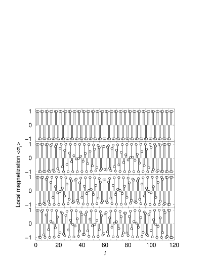
Figure 2: The local magnetization $\langle\sigma_{i}\rangle$ calculated for $L=118$ ($i=1,2,\dots,118$) with parallel and antiparallel boundary conditions.

We use dimensionless units $k_{\rm B}$ = $J_{1}$ = $1$ throughout this article. We focus on analysis of the model at $\kappa=0.6$, where the competing interaction plays an important role on the spin modulation. Figure 2 shows the local magnetization $\langle\sigma_{i}\rangle$ at $\kappa=0.6$ under and over a transition temperature $T_{\rm c}\approx 0.91$ which we will determine more precisely. The complete antiphase structure $\{\uparrow\uparrow\downarrow\downarrow\}$ is observed at $T=0.88$ if the parallel boundary conditions are imposed (the uppermost) and a twisted pattern created by a running domain wall is observed for the antiparallel conditions (the second from top). The remaining two panels display $\langle\sigma_{i}\rangle$ at $T=0.93$, where a modulated structure is present for the parallel conditions (the third panel) and the antiparallel ones (the fourth). Note that the modulation period depends on the applied boundary conditions.

3 Modulation Period

For the purpose of characterizing the spin modulation, we introduce the “domain-wall free energy” [21]

$${\cal F}_{\rm DW}(T,L)=(-1)^{n(L)}k_{\rm B}T\ln\frac{\lambda_{L}^{\uparrow\downarrow}(T)}{\lambda_{L}^{\uparrow\uparrow}(T)}\,,$$ (5)

where $n(L)=[L/2+2]+L+1$ represents the 4-site periodicity in the antiphase. The ${\cal F}_{\rm DW}(T,L)$ represents the sensitivity of the free energy per lattice row to the boundary conditions. In the antiphase region, ${\cal F}_{\rm DW}(T,L)$ exhibits the $L$ dependence

$${\cal F}_{\rm DW}(T,L)\sim{\cal F}_{\rm DW}(T,\infty)+c(T)L^{-2},$$ (6)

where $c(T)$ is a parameter, which is related to the ‘mass’ of the moving domain wall, and where ${\cal F}_{\rm DW}(T,\infty)$ represent the ‘stationary’ domain-wall energy. Figure 3 shows the dependence of ${\cal F}_{\rm DW}(T,\infty)$ with respect to $T$. The domain-wall free energy vanishes at critical temperature $T_{\rm c}^{\rm(A)}=0.907$; the superscript (A) stands for the fact that we have estimated the temperature inside the antiphase region.

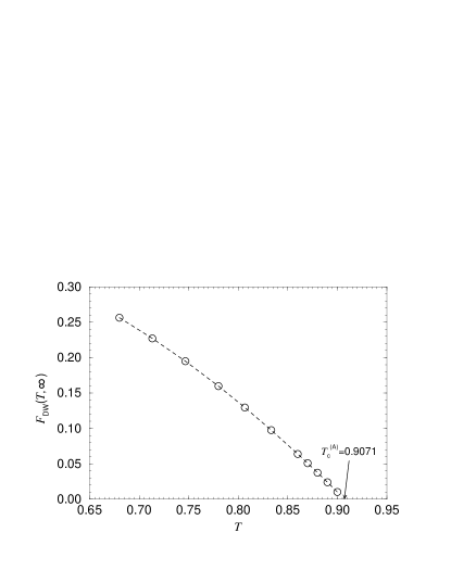
Figure 3: The domain-wall energy ${\cal F}_{\rm DW}(T,\infty)$ at $\kappa=0.6$.

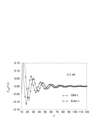
Figure 4: The domain-wall free energy with respect to size $L$ at $T=1.45$ and $\kappa=0.6$ (the symbols). The saw-like fitting functions are given by Eq. (8).

A detailed analysis of the ${\cal F}_{\rm DW}(T,L)$ is required in the higher temperature region ($T>T_{\rm c}$). The typical $L$-dependence of ${\cal F}_{\rm DW}(T,L)$ is depicted in Fig. 4. The saw-like structure in ${\cal F}_{\rm DW}(T,L)$ is naturally explained from the fact that the system prefers to have ‘a natural’ wave number $q(T)$ for the spin modulation if the system size is infinitely large ($L\to\infty$). When $L$ is finite, the boundary conditions force the system to have a modified wave number $q^{\prime}(T)$, which is quantized as

$$q^{\prime}_{\uparrow\uparrow}(T) = 2\pi m/(L-\ell)\,,$$

$$q^{\prime}_{\uparrow\downarrow}(T) = 2\pi(m+1)/(L-\ell)\,,$$ (7)

respectively, for the parallel and the antiparallel conditions, where $m$ is an appropriate integer and $\ell$ is an offset. As a consequence of the ‘forced’ shift in the wave number, a small increase of the free energy per site occurs and is proportional to ${[q(T)-q^{\prime}_{\uparrow\uparrow}(T)]}^{2}$ and ${[q(T)-q^{\prime}_{\uparrow\downarrow}(T)]}^{2}$ if higher-order corrections are omitted. Paying attention to the quantization condition in Eq. (7) and subtracting ${\cal F}_{\uparrow\uparrow}(T,L)=-k_{\rm B}T\ln\lambda_{L}^{\uparrow\uparrow}(T)$ from ${\cal F}_{\uparrow\downarrow}(T,L)=-k_{\rm B}T\ln\lambda_{L}^{\uparrow\downarrow}(T)$, we obtain the saw-like dependence in ${\cal F}_{\rm DW}(T,L)$ with respect to $L$ shown in Fig. 4. For the quantitative determination of $q(T)$, we employ a fitting function of the form

$${\cal F}_{\rm DW}(T,L)=\frac{ae^{-dL}}{L}\bigl{\{}\left|\cos(kL+\varphi)\right|-\left|\sin(kL+\varphi)\right|\bigr{\}}$$ (8)

that contains four temperature dependent parameters: $a$ is an amplitude, $\varphi$ is the phase offset which is related to $\ell$ in Eq. (7), $d$ is a dumping, and

$$k\equiv k(T)=q(T)-\pi/2$$ (9)

represents a change of the wave number $q(T)$ from the antiphase wave number $\pi/2$ [22]. (Precisely speaking, as shown in Fig. 4, there is a kind of even-odd oscillation, and we have to shift $\varphi$ in Eq. (8) by $\pi/4$ when $L$ is odd.) In Fig. 5, we plot $\bigl{[}k(T)\bigr{]}^{2}$ as a function of temperature $T$. Performing the extrapolation for $k(T)$, we obtain the critical temperature $T_{\rm c}^{\rm(P)}=0.907$, which is determined in the paramagnetic region. This result is in accordance with the previously obtained $T_{\rm c}^{\rm(A)}$. It should be noted that the linearity of $\bigl{[}k(T)\bigr{]}^{2}$ with respect to $T$ is in accordance with the free-fermionic picture on the spontaneously created domain walls. [7, 8].

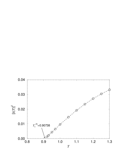
Figure 5: Behavior of the wave number $[k(T)]^{2}={[q(T)-\pi/2]}^{2}$.

Let us observe the temperature dependence of the decay factor $d(T)$. Figure 6 shows $d(T)$ in logarithmic scale. Since our survey is limited to $L\leq 118$, the estimated $d(T)$ for each temperature contains relatively large fitting error, which is visible as a fluctuation of the plotted data. Among the trial functions we have considered, the one

$$d(T)=\alpha\,\exp[-\beta(T-T_{\rm c}^{~{}})^{-1}_{~{}}]$$ (10)

shows the best fit when $\alpha=1.32(30)$, $\beta=2.17(32)$, and $T_{\rm c}^{~{}}=0.907(50)$. Though we don’t have any clear picture about the reason of the temperature dependence, the obtained $T_{\rm c}^{~{}}$ is in accordance with $T_{\rm c}^{(A)}$ and $T_{\rm c}^{(P)}$.

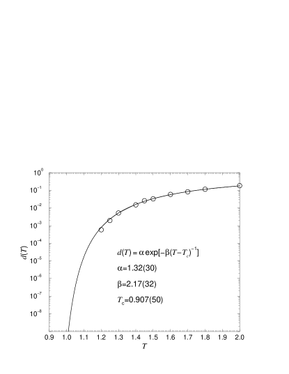
Figure 6: Temperature dependence of the dumping factor.

As an complementary approach, we calculate ${\cal F}_{\rm DW}(T,L)$ as a function of $T$ at $\kappa=0.6$ (see Fig. 7.) For simplicity we choose even $L$ in this calculation. Again, we obtain the saw-like dependence of ${\cal F}_{\rm DW}(T,L)$ which rapidly decays in higher temperature region. It is expected that the fitting function in Eq. (8) with the previously determined parameters $a$, $k$, $\varphi$, and $d$ explains the plotted data. The curve shown in Fig. 7 is thus drawn, and a good agreement is found between the plotted data and the fitting by Eq. (8).

Now, let us observe the ‘first zero-crossing temperature’ of ${\cal F}_{\rm DW}(T,L)$ from the low-temperature side, when $L$ is fixed. Speaking phenomenologically, the wave number in the thermodynamic limit $q(T)$ starts to deviate from $\pi/2$ at the critical temperature $T_{\rm c}$. Therefore for the finite size system the domain wall energy ${\cal F}_{\rm DW}(T,L)$ becomes zero when

$$[q(T)-\pi/2]L=k(T)L=\pi/2$$ (11)

is satisfied. Thus the zero-crossing temperature, say $T=T_{0}^{~{}}(L)$, is slightly larger than $T_{\rm c}^{~{}}$. From the analysis we have performed, we already know that $k(T)$ is proportional to $\sqrt{T-T_{\rm c}}$. Combined with Eq.(11), we get the relation

$$\sqrt{T-T_{0}^{~{}}(L)}\propto L^{-1}\,.$$ (12)

In order to confirm this, we plot the relative temperature

$$t=\frac{T_{0}^{~{}}(L)-T_{0}^{~{}}(\infty)}{T_{0}^{~{}}(\infty)}$$ (13)

with respect to $L^{-2}$ in Fig. 8, where $T_{0}^{~{}}(\infty)$ for each $\kappa$ is appropriately chosen so that the best linearity in the plotted data is realized. As a result, we obtain $T_{0}^{~{}}(\infty)=0.907$ at $\kappa=0.6$, which is in accordance with previously obtained transition temperatures.

For other values of $\kappa$ we obtain $T_{0}^{~{}}=1.335$ at $\kappa=0.8$, and $T_{0}^{~{}}=1.654$ at $\kappa=1.0$. The transition temperatures thus obtained are used for drawing the phase diagram shown in Fig. 1. It should be noted that the divergence of the correlation length at the transition temperature leads to the relation $t\propto L^{-1/\nu}$ [23], and from the relation we obtain a critical exponent $\nu=0.5$. This value is in accordance with the free-fermion picture [7, 24].

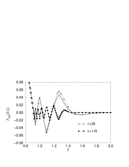
Figure 7: Dependence of ${\cal F}_{\rm DW}(T,L)$ on temperature $T$ at $\kappa=0.6$. The symbols with dotted lines represent the calculated ${\cal F}_{\rm DW}(T,L)$ and the full curves are drawn by Eq. (8).

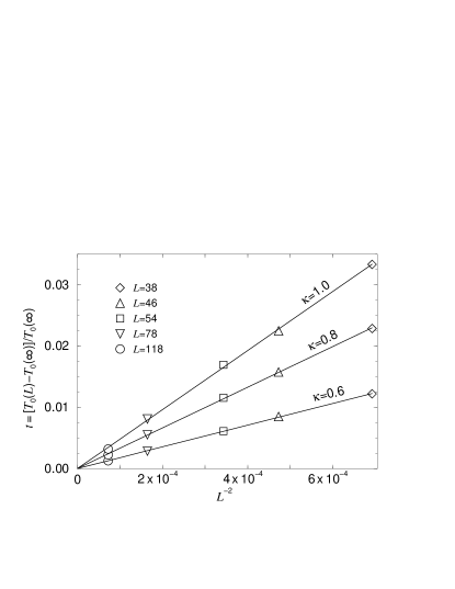
Figure 8: The relative temperature $t$ with respect to $L^{-2}$ for $\kappa=0.6$, $\kappa=0.8$, and $\kappa=1.0$.

4 Conclusions and Discussions

In conclusion, we have applied DMRG to the 2D ANNNI model. Observing the spin modulation period, we confirm that the free-fermion picture well describes the phase transition from the antiphase to the modulated state.

Since the correlation length is far longer than the size of systems in our study when the temperature is slightly higher than $T_{\rm c}$, we cannot directly judge whether there is a ‘stable’ IC phase or the modulated states are actually decaying in the long distance limit. At least we can say that we observe no conspicuous singularity in the modulation period above $T_{\rm c}$ as shown in Fig. 5. Comparing the fact with the possible temperature region for the IC phase reported by Shirahata and Nakamura [10], we conjecture that there is no IC phase in 2D ANNNI model, which is one of the possibility pointed by Shirahata and Nakamura.

This work is supported by the VEGA grants No. 2/6071/26 and No. 2/3118/23, and the Grant-in-Aid for Scientific Research from Ministry of Education, Science, Sports and Culture (No. 17540327).

References

- [1] M. Matsuda, K. Katsumata, T. Yokoo, S. M. Shapiro and G. Shirane Phys. Rev. B 54 (1996) R15626
- [2] H. F. Fong, B. Keimer, A. Hayashi and R. J. Cava Phys. Rev. B 59 (1999) 6873
- [3] J. Rossat-Mignot, P. Burlet, J. Villain, H. Bartholin, Wang Tcheng-Si, D. Florence and O. Vogt Phys. Rev. B 16 (1977) 440
- [4] Y. Yamada, I. Shibuya and S. Hoshino J. Phys. Soc. Jpn. 18 (1963) 1594
- [5] V. Massida and C.R. Mirasso Phys. Rev. B 40 (1989) 9327
- [6] W. Selke Phys. Rep. 170 (1988) 213
- [7] J. Villain and P. Bak J. Phys. (Paris) 42 (1981) 657
- [8] M.D. Grynberg and H. Ceva Phys. Rev. B 36 (1987) 7091
- [9] J. Kroemer and W. Pesch J. Phys. A 15 (1982) L25
- [10] T. Shirahata and T. Nakamura Phys. Rev. B 65 (2002) 024402
- [11] A. Gendiar and T. Nishino Phys. Rev. B 71 (2005) 024404
- [12] A. Gendiar and A. Šurda J. Phys. A: Math. Gen. 33 (2000) 8365
- [13] V. L. Berezinskii Sov. Phys. JETP 34 (1972) 610
- [14] J.M. Kosterlitz and D.J. Thouless J. Phys. C 6 (1973) 1181
- [15] A. Sato and F. Matsubara Phys. Rev. B 60 (1999) 10316
- [16] S. R. White Phys. Rev. Lett. 69 (1992) 2863
- [17] T. Nishino J. Phys. Soc. Jpn. 64 (1995) 3598
- [18] U. Schollwoeck Rev. Mod. Phys. 77 (2005) 259
- [19] M.A.S. Saqi and D.S. McKenzie J. Phys. A 20 (1987) 471
- [20] Y. Murai, K. Tanaka and T. Morita Physica A 217 (1995) 214
- [21] H.L. Richards, M.A. Novotny and P.A. Rikvold Phys. Rev. B 48 (1993) 14584
- [22] We show the details elsewhere
- [23] M. N. Barber Finite-size Scaling, vol. 8 (Academic Press 1983) 145–266
- [24] M.D. Grynberg and H. Ceva Phys. Rev. B 43 (1991) 13630