Single hole dynamics in the Kondo Necklace and Bilayer Heisenberg models on a square lattice.

Abstract

We study single hole dynamics in the bilayer Heisenberg and Kondo Necklace models. Those models exhibit a magnetic order-disorder quantum phase transition as a function of the interlayer coupling $J_{\bot}$. At strong coupling in the disordered phase, both models have a single-hole dispersion relation with band maximum at ${\boldsymbol{p}}=(\pi,\pi)$ and an effective mass at this ${\boldsymbol{p}}-$point which scales as the hopping matrix element $t$. In the Kondo Necklace model, we show that the effective mass at ${\boldsymbol{p}}=(\pi,\pi)$ remains finite for all considered values of $J_{\bot}$ such that the strong coupling features of the dispersion relation are apparent down to weak coupling. In contrast, in the bilayer Heisenberg model, the effective mass diverges at a finite value of $J_{\bot}$. This divergence of the effective mass is unrelated to the magnetic quantum phase transition and at weak coupling the dispersion relation maps onto that of a single hole doped in a planar antiferromagnet with band maximum at ${\boldsymbol{p}}=(\pi/2,\pi/2)$. We equally study the behavior of the quasiparticle residue in the vicinity of the magnetic quantum phase transition both for a mobile and static hole. In contrast to analytical approaches, our numerical results do not unambiguously support the fact that the quasiparticle residue of the static hole vanishes in the vicinity of the critical point. The above results are obtained with a generalized version of the loop algorithm to include single hole dynamics on lattice sizes up to $20\times 20$.

I Introduction

The modeling of heavy fermion systems is based on an array of localized spin degrees of freedom coupled antiferromagnetically to conduction electrons. Those models show competing interactions which lead to magnetic quantum phase transitions as a function of the antiferromagnetic exchange interaction $J$. Kondo screening of the localized spins, dominant at large $J$, favors a paramagnetic heavy fermion ground state, where the localized spins participate in the Luttinger volume. In contrast, the RKKY interaction favors magnetic ordering and is dominant at small values of $J$. There has recently been renewed interest concerning the understanding this quantum phase transition. In particular, recent Hall experiments Paschen04 suggest the interpretation that in the vicinity of the quantum phase transition the localized spins drop out of the Luttinger volume. Starting from the paramagnetic phase, this transition from a large to small Fermi surface should coincide with a effective mass divergence of the heavy fermion band.

Motivated by the above, we consider here a very simplified situation namely that of a doped hole in the Kondo insulating state as realized by the Kondo necklace and related models. Although this is not of direct relevance for the study of the Fermi surface, it does allow us to investigate the form of the quasiparticle dispersion relation from strong to weak coupling for a variety of models. Our aim here is two fold. On one hand we address the question of the divergence of the effective mass as a function of coupling for different models, and on the other hand the fate of the quasiparticle residue in the vicinity of the quantum phase transition.

The KLM emerges from the periodic Anderson model (PAM), where we have localized orbitals (LO) with on-site Hubbard interaction $U_{f}$ and extended orbitals (EO), which form a conduction band with dispersion $\varepsilon({\boldsymbol{p}})=-2t\left(\cos p_{x}+\cos p_{y}\right)$. The overlap between the LOs and the EOs within each unit cell is described by the hybridization matrix element $V$. For large $U_{f}$ charge fluctuations on the localized orbitals becomes negligible and the PAM maps via the Schrieffer-Wolff transformation onto the KLM Schrieffer66 ; Tsunetsugu97 :

$$\hat{H}_{\text{KLM}}=\sum_{{\boldsymbol{p}},\sigma}\varepsilon({\boldsymbol{p}})\hat{c}^{\dagger}_{{\boldsymbol{p}}\sigma}\hat{c}_{{\boldsymbol{p}}\sigma}+\mathcal{J}\sum_{i}\hat{{\boldsymbol{S}}}^{c}_{{\boldsymbol{i}}}\hat{{\boldsymbol{S}}}^{f}_{{\boldsymbol{i}}}\,\,.$$ (1)

Here $\hat{{\boldsymbol{S}}}^{c}_{{\boldsymbol{i}}}$ and $\hat{{\boldsymbol{S}}}^{f}_{{\boldsymbol{i}}}$ are spin $1/2$ operators for the extended orbitals and the localized orbitals respectively. In the first term, which represents the hopping processes, the fermionic operators $\hat{c}^{\dagger}_{{\boldsymbol{p}}\sigma}$ ($\hat{c}_{{\boldsymbol{p}}\sigma}$ ) create (annihilate) electrons in the conduction band with wave vector ${\boldsymbol{p}}$ and $z$-component of spin $\sigma$. At half-filling – one conduction electron per localized spin – the two-dimensional KLM is an insulator and shows a magnetic order-disorder quantum phase transition at a critical value of $\mathcal{J}_{c}/t=1.45\pm 0.05$ Capponi00 .

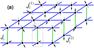
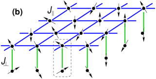
Figure 1: (a) Isotropic bilayer Heisenberg model. (b) Kondo Necklace model, that is related to the $U$KLM. In both cases the system dimerizes for large $J_{\bot}$, so that the AF ordering breaks down.

By taking into account an additional Coulomb repulsion $U$ between electrons within the conduction band, one obtains a modification of the KLM, the $U$KLM:

$$\hat{H}_{U\text{KLM}} = \sum_{{\boldsymbol{p}},\sigma}\varepsilon({\boldsymbol{p}})\hat{c}^{\dagger}_{{\boldsymbol{p}}\sigma}\hat{c}_{{\boldsymbol{p}}\sigma}+\mathcal{J}\sum_{i}\hat{{\boldsymbol{S}}}^{c}_{{\boldsymbol{i}}}\hat{{\boldsymbol{S}}}^{f}_{{\boldsymbol{i}}}$$ (2)

$$+U\sum_{{\boldsymbol{i}}}\left(\hat{n}_{{\boldsymbol{i}}\uparrow}-\tfrac{1}{2}\right)\left(\hat{n}_{{\boldsymbol{i}}\downarrow}-\tfrac{1}{2}\right)\,\,.$$

Here, $\hat{n}_{{\boldsymbol{i}}\sigma}=\hat{c}^{\dagger}_{{\boldsymbol{i}}\sigma}\hat{c}_{{\boldsymbol{i}}\sigma}$ is the density operator for electrons with spin $\sigma$ in the conduction band. The additional Coulomb repulsion displaces the quantum critical point towards smaller value of $\mathcal{J}_{c}/t$. However the physics, in particular the single hole dynamics, remains unchange Feldbacher02 . This allows us to take the limit $U/t\rightarrow\infty$ to map the UKLM onto a Kondo necklace model (KNM) which we write as:

$$\hat{H} = J_{\bot}\sum_{{\boldsymbol{i}}}\hat{{\boldsymbol{S}}}^{(1)}_{{\boldsymbol{i}}}\hat{{\boldsymbol{S}}}^{(2)}_{{\boldsymbol{i}}}+\sum_{\langle{\boldsymbol{i}}{\boldsymbol{j}}\rangle}\sum_{m}J^{(m)}_{\|}\hat{{\boldsymbol{S}}}^{(m)}_{{\boldsymbol{i}}}\hat{{\boldsymbol{S}}}^{(m)}_{{\boldsymbol{j}}}.$$ (3)

Here $\hat{{\boldsymbol{S}}}^{(m)}_{{\boldsymbol{i}}}$ is a spin $1/2$ operator, which acts on a spin degree of freedom at site ${\boldsymbol{i}}$. $J^{(m)}_{\|}$ stands for the intralayer exchange and the upper index $m=1,2$ labels the two different layers. The interlayer exchange, formerly the AF coupling $\mathcal{J}$ between LOs and EOs, is now characterized by $J_{\bot}$. Clearly, since we have motivated the KNM from a strong coupling limit of the UKLM, we have to set:

$$J^{(1)}_{\|}\equiv J_{\|}\quad J^{(2)}_{\|}=0\quad\text{for the KNM.}$$ (4)

The above models all have in common that the only interaction between the localized spins stems from the RKKY interaction. This in turn leads to the fact that at $\mathcal{J}=0$ for the KLM and UKLM or $J_{\bot}=0$ for the KNM the ground state is macroscopically degenerate. To lift the pathology we finally consider a Bilayer Heisenberg Model (BHM) in which an independent exchange between the localized spins is explicitly included in the Hamiltonian. Hence we will equally consider an Isotropic BHM which takes the form of Eq. (3) with:

$$J^{(1)}_{\|}=J^{(2)}_{\|}\equiv J_{\|}\quad\text{for the isotropic BHM.}$$ (5)

Both the KNM and BHM systems are sketched in FIG. 1.

The main results and organization of the paper are the following. In section II we give a short overview of the quantum Monte Carlo (QMC) method. We use a generalization of the loop algorithm which allows for the calculation of the imaginary time Green’s function of the doped hole Brunner00 . Dynamical information is obtained with a stochastic Maximum Entropy method Beach04 ; Sandvik98 . In the first part of section III we present our results for the spin dynamics. This includes the determination of the quantum critical point for the isotropic BHM as well as the Kondo Necklace model (KNM) by QMC methods. In the second part of that section we analyze the single particle spectral function. It turns out, that there are significant differences between the models. We can identify two classes of models: In the isotropic BHM the dispersion is continously deformed with decreasing interplanar coupling $J_{\bot}/J_{\|}$ resulting in a displacement of the maximum from ${\boldsymbol{p}}=(\pi,\pi)$ to ${\boldsymbol{p}}=(\tfrac{\pi}{2},\tfrac{\pi}{2})$. In other words, the effective mass – as defined by the inverse curvature of the quasiparticle dispersion relation – at ${\boldsymbol{p}}=(\pi,\pi)$ diverges at a finite value of the interplanar coupling. This divergence of the effective mass is not related to the magnetic order-disorder transition. In contrast, in the KLM related models, UKLM and KNM, the maximum of the quasiparticle dispersion relation is pinned at ${\boldsymbol{p}}=(\pi,\pi)$ irrespective of the value of the interplanar coupling. In those models the effective mass at ${\boldsymbol{p}}=(\pi,\pi)$ grows as a function of decreasing interplanar coupling, but remains finite.

In section IV we turn to the analysis of the quasi particle residue (QPR) across the quantum phase transition. To gain intuition, we first carry out an approximate calculation in the lines of Ref. Sushkov00 . The physics of the spin system may be solved in the framework of a bond mean-field calculation. Here, the disordered phase is described in terms of a condensate of singlets between the planes and gaped spin 1 excitations (magnons). At the critical point the magnons condense at the AF wave vector thus generating the static antiferromagnetic order. Within this framework one can compute the coupling of the mobile hole with the magnetic fluctuations and study the hole dynamics within a self-consistent Born approximation. The result of the calculation shows that the quasiparticle weight at wave vectors on the magnetic Brillouin zone [$\epsilon({\boldsymbol{p}})=\epsilon({\boldsymbol{p}}+{\boldsymbol{Q}})$ with $\boldsymbol{Q}=(\pi,\pi)$ ] vanish as the square root of the spin gap. In contrast the QMC determination of the quasiparticle residue on lattices up to $20\times 20$ for static and dynamical holes does not unambiguously support this point of view.

II Numerical Methods

We use the world line QMC method with loop updates Evertz97 to investigate the physics of the BHM and KNM. To investigate the spin dynamics we compute both the spin stiffness as well as the dynamical spin structure factor. Our analysis of the single hole dynamics is based on the calculation of the imaginary time Green’s function. Analytical continuation with the use of the stochastic Maxent Method provides the spectral function and the quasiparticle residue is extracted from the asymptotic behavior of the imaginary time Green’s function. Below, we discuss in more details the calculation of each observables.

Spin Stiffness

To probe for long-ranged magnetic order we introduce a continuous twist in spin space which, when cumulated along the length $L$ along (e.g.) the $x$-axis, amounts to a twist of angle $\phi$ around a certain spin axis ${\boldsymbol{e}}$. This means thus the boundary conditions read: $\hat{{\boldsymbol{S}}}_{{\boldsymbol{i}}+L{\boldsymbol{e}}_{x}}=R\left[{\boldsymbol{e}},\phi\right]\hat{{\boldsymbol{S}}}_{{\boldsymbol{i}}}$, where $R\left[{\boldsymbol{e}},\phi\right]$ is a matrix describing an $SO(3)$ rotation around the axis ${\boldsymbol{e}}$ by the angle $\phi$. The spin stiffness is then defined as

$$\rho_{s}=\left.-\frac{1}{L^{d-2}}\frac{1}{\beta}\frac{\partial^{2}}{\partial\phi^{2}}\ln Z(\phi)\right|_{\phi=0}$$ (6)

with $\beta$ as inverse temperature, $L$ as the linear size of the system, $d$ the dimensionality and $Z(\phi)$ the twist dependent partition function. In the presence of long-range order $\rho_{s}$ takes a finite value and in a disordered phase it vanishes.

Within the world-line algorithm, the spin stiffness is related to the winding number $\mathcal{W}_{x}$ of the world line configurations along the axis of cumulatively twisted spins (e.g. $x$-axis). In particular, in the limit $\Delta\tau\to 0$ it takes the simple form

$$\rho_{s}=\frac{1}{L^{d}}\frac{1}{\beta}\mathcal{W}^{2}_{x}.$$ (7)

Spin Correlations

Within the QMC it is easy to obtain the spin correlations $\langle S^{z}_{{\boldsymbol{i}}}(\tau)S^{z}_{{\boldsymbol{j}}}(0)\rangle$ in real space and imaginary time $\tau$, where the imaginary time evolution of the spin operator reads $S^{z}_{{\boldsymbol{q}}}(\tau)=e^{\tau\hat{H}}S^{z}_{{\boldsymbol{q}}}e^{-\tau\hat{H}}$. Its representation in momentum space is related to the dynamical spin susceptibility $S({\boldsymbol{q}},\omega)$ via:

$$\langle S^{z}_{{\boldsymbol{q}}}(\tau)S^{z}_{-{\boldsymbol{q}}}(0)\rangle=\frac{1}{\pi}\int d\omega e^{-\tau\omega}S({\boldsymbol{q}},\omega).$$ (8)

By using the Stochastic Maximum Entropy (ME) method Beach04 we can extract the dynamical spin susceptibility. For large $\tau$ the spin correlation function is dominated by the lowest excitation:

$$\underset{\tau\rightarrow\infty}{\lim}\langle S^{z}_{{\boldsymbol{q}}}(\tau)S^{z}_{-{\boldsymbol{q}}}(0)\rangle\propto e^{-\Omega({\boldsymbol{q}})\tau}$$ (9)

where $\Omega({\boldsymbol{q}})$ stands for momentum dependent gap to the first spin excitation. Thus, we obtain the gap energy $\Delta$ from the asymptotic behavior of the spin correlations: $\Delta\equiv\min\left[\Omega({\boldsymbol{q}})\right]$.

The Green’s Function

To incorporate the dynamics of a single hole into the KNM and BHM, we consider the $tJ$-model

$$\hat{H}_{tJ} = \mathcal{P}_{S}\Big{[}-\sum_{\langle{\boldsymbol{i}}{\boldsymbol{j}}\rangle,\sigma}t_{\boldsymbol{i}\boldsymbol{j}}(\hat{c}^{\dagger}_{{\boldsymbol{i}}\sigma}\hat{c}_{{\boldsymbol{j}}\sigma}+\hat{c}^{\dagger}_{{\boldsymbol{j}}\sigma}\hat{c}_{{\boldsymbol{i}}\sigma})$$ (10)

$$+\displaystyle\sum_{\langle{\boldsymbol{i}}{\boldsymbol{j}}\rangle}J_{\boldsymbol{i}\boldsymbol{j}}\big{\{}\hat{{\boldsymbol{S}}}_{{\boldsymbol{i}}}\hat{{\boldsymbol{S}}}_{{\boldsymbol{j}}}-\tfrac{1}{4}\hat{n}_{{\boldsymbol{i}}}\hat{n}_{{\boldsymbol{j}}}\big{\}}\Big{]}\mathcal{P}_{S}$$

which describes the more general case of arbitrary filling. Here, ${\boldsymbol{i}}$ and ${\boldsymbol{j}}$ denote lattice sites of the bilayer BHM, $t_{{\boldsymbol{i}}{\boldsymbol{j}}}$ the hopping amplitude, $J_{{\boldsymbol{i}}{\boldsymbol{j}}}$ the exchange, $\hat{n}_{{\boldsymbol{j}}}=\hat{c}^{\dagger}_{{\boldsymbol{i}}\sigma}\hat{c}_{{\boldsymbol{i}}\sigma}$, and the sums run over nearest inter- and intraplane neighbors. Finally $\mathcal{P}_{S}$ is a projection operator onto the subspace $S$ with no double occupation. We apply a mapping, introduced by Angelucci Angelucci95 , which separates the spin degree of freedom and the occupation number.

$$\begin{array}[]{lcrclcl}|\uparrow\rangle&\longrightarrow&|1,\Uparrow\rangle&\hphantom{xxx}&\hat{c}_{{\boldsymbol{i}}\uparrow}&\longrightarrow&\hat{\sigma}^{z,+}_{{\boldsymbol{i}}}\hat{f}^{\dagger}_{{\boldsymbol{i}}}-\hat{\sigma}^{z,-}_{{\boldsymbol{i}}}\hat{f}_{{\boldsymbol{i}}}\vphantom{\frac{1}{1}}\\ |\downarrow\rangle&\longrightarrow&|1,\Downarrow\rangle&\hphantom{xxx}&\hat{c}^{\dagger}_{{\boldsymbol{i}}\uparrow}&\longrightarrow&\hat{\sigma}^{z,+}_{{\boldsymbol{i}}}\hat{f}_{{\boldsymbol{i}}}-\hat{\sigma}^{z,-}_{{\boldsymbol{i}}}\hat{f}^{\dagger}_{{\boldsymbol{i}}}\vphantom{\frac{1}{1}}\\ |0\rangle&\longrightarrow&|0,\Uparrow\rangle&\hphantom{xxx}&\hat{c}_{{\boldsymbol{i}}\downarrow}&\longrightarrow&(\hat{f}_{{\boldsymbol{i}}}+\hat{f}^{\dagger}_{{\boldsymbol{i}}})\hat{\sigma}^{+}_{{\boldsymbol{i}}}\vphantom{\frac{1}{1}}\\ |\uparrow\downarrow\rangle&\longrightarrow&|0,\Downarrow\rangle&\hphantom{xxx}&\hat{c}^{\dagger}_{{\boldsymbol{i}}\downarrow}&\longrightarrow&\hat{\sigma}^{-}_{{\boldsymbol{i}}}(\hat{f}^{\dagger}_{{\boldsymbol{i}}}+\hat{f}_{{\boldsymbol{i}}})\vphantom{\frac{1}{1}}\end{array}$$ (15)

$\hat{f}^{\dagger}_{{\boldsymbol{i}}}$ and $\hat{f}_{{\boldsymbol{i}}}$ are spinless fermion operators which act on the charge degree of freedom and create (annihilate) a hole at site $i$: $\hat{f}^{\dagger}_{{\boldsymbol{i}}}|1,\sigma\rangle=|0,\sigma\rangle$, $\hat{\sigma}^{\pm}_{{\boldsymbol{i}}}$ are ladder operators for the spin degree of freedom and $\hat{\sigma}^{z,\pm}_{{\boldsymbol{i}}}=\frac{1}{2}(1\pm\hat{\sigma}^{z}_{{\boldsymbol{i}}})$ are projector operators acting on the spin degree of freedom. Within this base the Hamilton of the $tJ$-model (10) writes:

$$\tilde{H}_{tJ} = \tilde{\mathcal{P}}_{S}\Big{[}\sum_{\langle{\boldsymbol{i}}{\boldsymbol{j}}\rangle}t_{{\boldsymbol{i}}{\boldsymbol{j}}}\big{[}\hat{f}^{\dagger}_{{\boldsymbol{j}}}\hat{f}_{{\boldsymbol{i}}}\tilde{P}_{{\boldsymbol{i}}{\boldsymbol{j}}}+\mathrm{h.c.}\big{]}$$ (16)

$$+\frac{1}{2}\sum_{\langle{\boldsymbol{i}}{\boldsymbol{j}}\rangle}J_{{\boldsymbol{i}}{\boldsymbol{j}}}(\tilde{P}_{{\boldsymbol{i}}{\boldsymbol{j}}}-1)\tilde{\Delta}_{{\boldsymbol{i}}{\boldsymbol{j}}}\Big{]}\tilde{\mathcal{P}}_{S}$$

where $\tilde{P}_{{\boldsymbol{i}}{\boldsymbol{j}}}=\tfrac{1}{2}(\hat{\vec{\sigma}}_{{\boldsymbol{i}}}\hat{\vec{\sigma}}_{{\boldsymbol{j}}}+1)$ and $\tilde{\Delta}_{{\boldsymbol{i}}{\boldsymbol{j}}}=1-\hat{f}^{\dagger}_{{\boldsymbol{i}}}\hat{f}_{{\boldsymbol{i}}}-\hat{f}^{\dagger}_{j}\hat{f}_{{\boldsymbol{j}}}$ $\tilde{\mathcal{P}}_{S}=\prod_{{\boldsymbol{i}}}\big{(}1-\hat{f}^{\dagger}_{{\boldsymbol{i}}}\hat{f}_{{\boldsymbol{i}}}\hat{\sigma}^{-}_{{\boldsymbol{i}}}\hat{\sigma}^{+}_{{\boldsymbol{i}}}\big{)}$ is a projection operator in Angelucci representation which projects into the subspace $S$. This representation (16) has two important advantages which facilitate numerical simulations: (i) Because the Hamiltonian commutes with the projection operator: $[\tilde{H}_{tJ},\tilde{\mathcal{P}}_{S}]=0$, the bare Hamiltonian ($\tilde{H}_{tJ}$ without projections) generates only states of subspace $S$ provided that the initial state is in the relevant subspace. (ii) The Hamiltonian is bilinear in the spinless fermion operators. Within the Angelucci representation the Green’s function reads:

$$G_{{\boldsymbol{j}}{\boldsymbol{i}}}(\tau)=\langle\hat{\sigma}^{z,+}_{{\boldsymbol{j}}}(\tau)\hat{f}_{{\boldsymbol{j}}}(\tau)\hat{\sigma}^{z,+}_{{\boldsymbol{i}}}(0)\hat{f}^{\dagger}_{{\boldsymbol{i}}}(0)\rangle\,\,.$$ (17)

The time evolution in imaginary time is given by: $\hat{\sigma}^{z,+}_{{\boldsymbol{j}}}(\tau)\hat{f}_{{\boldsymbol{j}}}(\tau)=e^{\tau\tilde{H}_{tJ}}\hat{\sigma}^{z,+}_{{\boldsymbol{j}}}\hat{f}_{{\boldsymbol{j}}}e^{-\tau\tilde{H}_{tJ}}$. The authors of Ref. Brunner00 show in details how to implement the Green’s function into the world line algorithm of our QMC simulation. The spin dynamics is simulated with the loop algorithm. For each fixed spin configuration, one can readily compute the Green’s function since the Hamiltonian is bilinear in the spinless fermion operators $\hat{f}$.

From the Green’s function $G_{{\boldsymbol{p}}}(\tau)$ we can extract the single particle spectral function $A({\boldsymbol{p}},\omega)$ with the Stochastic Maximum Entropy:

$$G_{{\boldsymbol{p}}}(\tau)=\frac{1}{\pi}\int^{\infty}_{0}d\omega e^{-\tau\omega}A({\boldsymbol{p}},-\omega)\,\,.$$ (18)

In the $T=0$ limit the asymptotic form of the Green’s function reads:

$$G_{{\boldsymbol{p}}}(\tau)=|\langle\psi^{N-1}_{0}|\hat{c}_{{\boldsymbol{p}}}|\psi^{N}_{0}\rangle|^{2}e^{-\mu\tau}$$ (19)

where $\mu$ is the chemical potential. As apparent, the prefactor,

$$\mathcal{Z}_{\boldsymbol{p}}=|\langle\psi^{N-1}_{0}|\hat{c}_{{\boldsymbol{p}}}|\psi^{N}_{0}\rangle|^{2}\,\,,$$ (20)

is nothing but the quasiparticle residue. Hence from the asymptotic form of the single particle Green’s function, we can read off the quasiparticle residue.

III Spin and Hole Dynamics

In this section we present our results for the spin dynamics as well as for the spectral function of a doped mobile hole.

III.1 Spin Dynamics

All considered models, KLM, $U$KLM, KNM and BHM, show a quantum phase transition between an antiferromagnetic ordered phase and a disordered phase. It is believed, that all models belong to the same universality class. To demonstrate this generic property and to test our numerical method we determine the quantum critical point as well as critical exponents in the isotropic BHM and KNM. Fig. 2a plots the spin stiffness for the KNM as a function of lattice size.

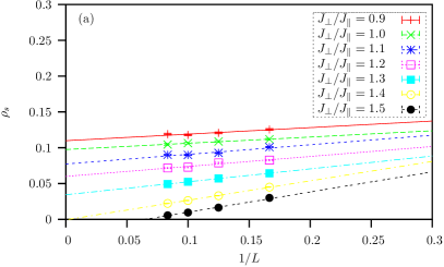
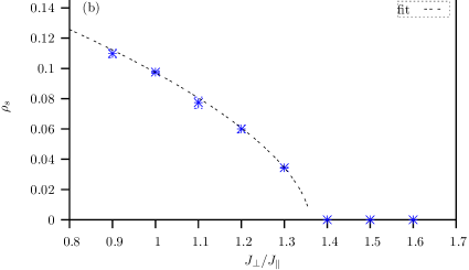
Figure 2: (a) Spin stiffness $\rho_{s}$ as a function of linear lattice size $L$ for different interplanar couplings $J_{\bot}/J_{\|}$ in the KN model. Extrapolation to the thermodynamic limit is carried out by fitting to the form $a+b/L$ (b) Extrapolated value of the spin stiffness as a function of $J_{\bot}/J_{\|}$. The dashes line corresponds to the fit according to the form of Eq. (21).

The extrapolated data is plotted in Fig. 2b. We fit the data to the form:

$$\rho_{s}\propto\Big{[}\Big{(}\frac{J_{\bot}}{J_{\|}}\Big{)}_{c}-\Big{(}\frac{J_{\bot}}{J_{\|}}\Big{)}\Big{]}^{\nu}\,\,$$ (21)

to obtain $(J_{\bot}/J_{\|})_{c}=1.360\pm 0.017$ and a critical exponent of $\nu=0.582\pm 0.077$, which agrees (within the error bars) with the value of Ref. Troyer97 : $\nu=0.685\pm 0.035$. Similar data for the BHM localizes the quantum critical point at $(J_{\bot}/J_{\|})_{c}=2.5121\pm 0.0044$, which conforms roughly the literature value $(J_{\bot}/J_{\|})^{lit}_{c}=2.525\pm 0.002$ of Ref. Shevchenko00 . For the critical exponent we obtain $\nu=0.7357\pm 0.044$. Again this is in good agreement with the critical exponent specified in Refs. Troyer97 . In Ref. Kotov98 the BHM and the KNM are observed by dimer series expansions. Within this framework our numerical results are reflected quite well. FIG. 3 plot the dynamical spin structure factor as a function of $J_{\bot}/J_{\|}$ for the BHM. In the deeply disordered phase the dispersion has a cosine-like shape. In the limit $J_{\bot}\to\infty$ the ground state wave function is a tensor product of singlets in each unit cell. Starting from this state, a magnon corresponds to breaking a singlet to form a triplet. In first order perturbation theory in $J_{\bot}/J_{\|}$, the magnon acquires a dispersion relation:

$$\Omega({\boldsymbol{q}})\approx J_{\bot}+\tfrac{1}{2}J_{\|}\gamma({\boldsymbol{q}})$$ (22)

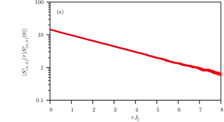
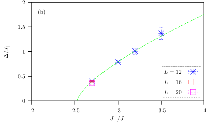
Figure 4: (a) Spin correlation function ($J_{\bot}/J_{\|}=2.7$) at ${\boldsymbol{p}}=(\pi,\pi)$ for a $12\times 12$ lattice in the BHM. (Inverse temperature $\beta J_{\|}=30.0$, $\Delta\tau J_{\|}=0.02$) (b) Spin gap $\Delta$ at ${\boldsymbol{p}}=(\pi,\pi)$ for different coupling ratios $J_{\bot}/J_{\|}$. The data for a $12\times 12$ lattice is fitted by $\Delta\propto\left(g-g_{c}\right)^{-z\nu}$ with $g=J_{\bot}/J_{\|}$ and literature values $g_{c}=2.525\pm 0.002$ Shevchenko00 and $z=1$ Troyer97

with $\gamma({\boldsymbol{q}})=2\left(\cos(q_{x})+\cos(q_{y})\right)$. This approximative approach is roughly consistent with the large-$J_{\bot}$ case in Fig. 3a. As as function of decreasing coupling $J_{\bot}$ the spin gap progressively closes (see Fig. 4) and at the critical coupling the magnons at ${\boldsymbol{q}}=(\pi,\pi)$ condense to form the antiferromagnetic order. This physics is captured by the bond mean field approximation which we discuss below.

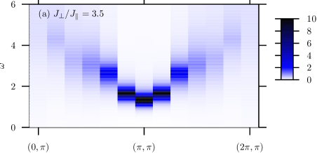
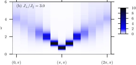
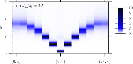
${\boldsymbol{q}}$

Figure 3: Dynamical spin susceptibility, respectively magnon dispersion for different coupling ratios on a $12\times 12$ square lattice.

Bond Operator Mean Field Approach

The bond mean field approach Sachdev90 is a strong coupling approximation in $J_{\bot}$. The spins between layers dominantly form singlets and the density of triplets is ”low”. This assumption allows one to neglect triplet-triplet interaction. The bond operator representation describes the system in a base of pairs of coupled spins, which can either be in a singlet or triplet state.

$$|s\rangle_{{\boldsymbol{i}}} = \hat{s}^{\dagger}_{{\boldsymbol{i}}}|0\rangle_{{\boldsymbol{i}}}=\frac{1}{\sqrt{2}}(|\uparrow\downarrow\rangle_{{\boldsymbol{i}}}-|\downarrow\uparrow\rangle_{{\boldsymbol{i}}})$$

$$|t_{x}\rangle_{{\boldsymbol{i}}} = \hat{t}^{\dagger}_{{\boldsymbol{i}}x}|0\rangle_{{\boldsymbol{i}}}=\frac{-1}{\sqrt{2}}(|\uparrow\uparrow\rangle_{{\boldsymbol{i}}}-|\downarrow\downarrow\rangle_{{\boldsymbol{i}}})$$

$$|t_{y}\rangle_{{\boldsymbol{i}}} = \hat{t}^{\dagger}_{{\boldsymbol{i}}y}|0\rangle_{{\boldsymbol{i}}}=\frac{\mathrm{i}}{\sqrt{2}}(|\uparrow\uparrow\rangle_{{\boldsymbol{i}}}+|\downarrow\downarrow\rangle_{{\boldsymbol{i}}})$$

$$|t_{z}\rangle_{{\boldsymbol{i}}} = \hat{t}^{\dagger}_{{\boldsymbol{i}}z}|0\rangle_{{\boldsymbol{i}}}=\frac{1}{\sqrt{2}}(|\uparrow\downarrow\rangle_{{\boldsymbol{i}}}+|\downarrow\uparrow\rangle_{{\boldsymbol{i}}})$$ (23)

The operators $\hat{t}^{\dagger}$ and $\hat{s}^{\dagger}$ satisfy Bose commutation rules provided that we impose the constraint

$$\hat{s}^{\dagger}_{{\boldsymbol{i}}}\hat{s}_{{\boldsymbol{i}}}+\sum_{\alpha}\hat{t}^{\dagger}_{{\boldsymbol{i}}\alpha}\hat{t}_{{\boldsymbol{i}}\alpha}=1\,\,.$$ (24)

Since the original spin 1/2 degrees of freedom reads,

$$\hat{S}^{(1,2)}_{{\boldsymbol{i}}\alpha} = \tfrac{1}{2}(\pm\hat{s}^{\dagger}_{{\boldsymbol{i}}}\hat{t}_{{\boldsymbol{i}}\alpha}\pm\hat{t}^{\dagger}_{{\boldsymbol{i}}\alpha}\hat{s}_{{\boldsymbol{i}}}-\mathrm{i}\sum_{\beta\gamma}\epsilon_{\alpha\beta\gamma}\hat{t}^{\dagger}_{{\boldsymbol{i}}\beta}\hat{t}_{{\boldsymbol{i}}\gamma})\,\,,$$ (25)

the Hamiltonian (3) can be rewritten in the bond operator representation as:

$$\tilde{H} = J_{\bot}\sum_{{\boldsymbol{i}}}\big{(}-\tfrac{3}{4}\hat{s}^{\dagger}_{{\boldsymbol{i}}}\hat{s}_{{\boldsymbol{i}}}+\tfrac{1}{4}\sum_{\alpha}\hat{t}^{\dagger}_{{\boldsymbol{i}}\alpha}\hat{t}_{{\boldsymbol{i}}\alpha}\big{)}$$

$$-\sum_{{\boldsymbol{i}}}\mu_{{\boldsymbol{i}}}\big{(}\hat{s}^{\dagger}_{{\boldsymbol{i}}}\hat{s}_{{\boldsymbol{i}}}+\sum_{\alpha}\hat{t}^{\dagger}_{{\boldsymbol{i}}\alpha}\hat{t}_{{\boldsymbol{i}}\alpha}-1\big{)}$$

$$+\frac{J_{\|}}{2}\sum_{\langle{\boldsymbol{i}}{\boldsymbol{j}}\rangle}\sum_{\alpha}\big{(}\hat{s}^{\dagger}_{{\boldsymbol{i}}}\hat{s}^{\dagger}_{{\boldsymbol{j}}}\hat{t}_{{\boldsymbol{i}}\alpha}\hat{t}_{{\boldsymbol{j}}\alpha}+\hat{s}^{\dagger}_{{\boldsymbol{i}}}\hat{s}_{{\boldsymbol{j}}}\hat{t}_{{\boldsymbol{i}}\alpha}\hat{t}^{\dagger}_{{\boldsymbol{j}}\alpha}+\mathrm{h.c.}\big{)}$$

$$+\frac{J_{\|}}{2}\sum_{\alpha,\beta,\gamma}(\hat{t}^{\dagger}_{{\boldsymbol{i}}\beta}\hat{t}_{{\boldsymbol{i}}\gamma}\hat{t}^{\dagger}_{{\boldsymbol{j}}\beta}\hat{t}_{{\boldsymbol{j}}\gamma}-\hat{t}^{\dagger}_{{\boldsymbol{i}}\beta}\hat{t}_{{\boldsymbol{i}}\gamma}\hat{t}^{\dagger}_{{\boldsymbol{j}}\gamma}\hat{t}_{{\boldsymbol{j}}\beta})\,\,.$$

$\mu_{{\boldsymbol{i}}}$ is a Lagrange parameter which enforces locally the constraint (24). The interplanar part shows the characteristic Hamiltonian of two antiferromagnetically coupled spins whereas the intraplanar part includes the interaction between singlets and triplets of different bonds. We now follow the standard method of Sachdev and Bhatt Sachdev90 . In the disordered phase we expect a singlet condensate ($\bar{s}=\langle s\rangle\neq 0$) and impose the constraint only on average ($\mu_{\boldsymbol{i}}=\mu$). As mentioned above we neglect triplet-triplet interactions. Apart from a constant we obtain the following mean field Hamiltonian in momentum space:

$$\hat{H}_{MFA} = \sum_{\alpha}\sum_{{\boldsymbol{q}}}A_{\boldsymbol{q}}\hat{t}^{\dagger}_{{\boldsymbol{q}}\alpha}\hat{t}_{{\boldsymbol{q}}\alpha}$$ (26)

$$+\sum_{\alpha}\sum_{{\boldsymbol{q}}}\frac{B_{\boldsymbol{q}}}{2}(\hat{t}^{\dagger}_{{\boldsymbol{q}}\alpha}\hat{t}^{\dagger}_{-{\boldsymbol{q}}\alpha}+\mathrm{h.c.})\,\,,$$

where

$$A_{\boldsymbol{q}} = \frac{J_{\bot}}{4}-\mu+J_{\|}\bar{s}^{2}\big{(}\cos(q_{x})+\cos(q_{y})\big{)}$$ (27)

$$B_{\boldsymbol{q}} = J_{\|}\bar{s}^{2}\big{(}\cos(q_{x})+\cos(q_{y})\big{)}\,\,.$$ (28)

The parameter $\mu$ and $\bar{s}=\langle s\rangle$ are determined by the saddle-point equations: $\langle\partial\hat{H}_{MFA}/\partial\mu\rangle=0$ and $\langle\partial\hat{H}_{MFA}/\partial\bar{s}\rangle=0$. The Hamiltonian is diagonalized by a Bogoliubov transformation: $\hat{\alpha}^{\dagger}_{{\boldsymbol{q}}\alpha}=u_{{\boldsymbol{q}}}\hat{t}^{\dagger}_{{\boldsymbol{q}}\alpha}-v_{{\boldsymbol{q}}}\hat{t}_{-{\boldsymbol{q}}\alpha}$. In terms of magnon creation and annihilation operators the Mean field Hamiltonian (26) writes:

$$\hat{H}_{MFA}=\sum_{\boldsymbol{q}}\sum_{\alpha}\Omega({\boldsymbol{q}})\hat{\alpha}^{\dagger}_{{\boldsymbol{q}}\alpha}\hat{\alpha}_{{\boldsymbol{q}}\alpha}\,\,.$$ (29)

The Bogoliubov coefficients $u_{{\boldsymbol{q}}}$ and $v_{{\boldsymbol{q}}}$ satisfy the relation $u^{2}_{{\boldsymbol{q}}}-v^{2}_{{\boldsymbol{q}}}=1$, which follows from the bosonic nature of the magnons: $[\hat{\alpha}_{{\boldsymbol{q}}},\hat{\alpha}^{\dagger}_{{\boldsymbol{q}}^{\prime}}]=\delta_{{\boldsymbol{q}}{\boldsymbol{q}}^{\prime}}$. The coefficients are given by

$$u_{{\boldsymbol{q}}},v_{{\boldsymbol{q}}} = \sqrt{\frac{A_{\boldsymbol{q}}}{2\Omega({\boldsymbol{q}})}\pm\frac{1}{2}}\,\,,$$ (30)

where $\Omega({\boldsymbol{q}})=\sqrt{A^{2}_{\boldsymbol{q}}-B^{2}_{\boldsymbol{q}}}$ is the magnon dispersion. In the vicinity of the critical point it can be approximated by

$$\Omega({\boldsymbol{q}})=\sqrt{\Delta^{2}+v^{2}_{s}({\boldsymbol{q}}-{\boldsymbol{Q}})^{2}}$$ (31)

with $\Delta$ the energy gap to magnon excitations, $v_{s}$ the magnon velocity and ${\boldsymbol{Q}}=(\pi,\pi)$. Eq. (31) gives an accurate description of the dispersion relation in the vicinity of the critical point (see FIG. 3c). At the critical point the gap $\Delta$ vanishes, so that the triplets can condense thus forming the AF static ordering.

III.2 Hole dynamics

We now dope our systems with a single mobile hole and restrict its motion to one layer thereby staying in the spirit of Kondo lattice models. To understand the coupling of the hole to magnetic fluctuations within the magnetic disordered phase we can extend the previously described bond mean-field approximation (See Eq. (29)) to account for the hole motion. For this we introduce the operator $\hat{h}^{\dagger}_{{\boldsymbol{i}}\sigma}$ ($\hat{h}_{{\boldsymbol{i}}\sigma}$), that creates (anhilates) a hole with spin $\sigma$ in layer 1 at site ${\boldsymbol{i}}$.

$$\hat{h}^{\dagger}_{{\boldsymbol{i}}\sigma}|vac\rangle = |0\sigma\rangle_{{\boldsymbol{i}}}$$ (32)

$|\sigma_{1}\sigma_{2}\rangle_{\boldsymbol{i}}$ denotes a dimer state at site ${\boldsymbol{i}}$ with spin $\sigma_{1}$ in layer 1 and spin $\sigma_{2}$ in layer 2. The Hamiltonian now writes Vojta99 :

$$\hat{H} = \sum_{{\boldsymbol{q}}}\Omega({\boldsymbol{q}})\hat{{\boldsymbol{\alpha}}}^{\dagger}_{{\boldsymbol{q}}}\hat{{\boldsymbol{\alpha}}}_{{\boldsymbol{q}}}+\sum_{{\boldsymbol{p}}}\varepsilon({\boldsymbol{p}})\hat{h}^{\dagger}_{{\boldsymbol{p}}}\hat{h}_{{\boldsymbol{p}}}$$

$$+\sum_{{\boldsymbol{p}},{\boldsymbol{q}}}g({\boldsymbol{p}},{\boldsymbol{q}})\,{\boldsymbol{\alpha}}_{\boldsymbol{q}}\cdot\big{(}\hat{h}^{\dagger}_{{\boldsymbol{p}}+{\boldsymbol{q}}}{\boldsymbol{\sigma}}\hat{h}_{{\boldsymbol{p}}}\big{)}+\text{h.c.}$$

with spinor $\hat{h}_{{\boldsymbol{p}}}=(\hat{h}_{{\boldsymbol{p}}\uparrow},\hat{h}_{{\boldsymbol{p}}\downarrow})$ and vector $\hat{{\boldsymbol{\alpha}}}_{{\boldsymbol{q}}}=(\hat{\alpha}_{{\boldsymbol{q}}x},\hat{\alpha}_{{\boldsymbol{q}}y},\hat{\alpha}_{{\boldsymbol{q}}z})$. ${\boldsymbol{\sigma}}=(\sigma^{1},\sigma^{2},\sigma^{3})$ denotes the Pauli matrices. The coupling strength between the hole and magnons is given by $g({\boldsymbol{p}},{\boldsymbol{q}})$. We discuss $g({\boldsymbol{p}},{\boldsymbol{q}})$ in detail later in section IV. For the bare hole dispersion the calculation yields

$$\varepsilon({\boldsymbol{p}})=+t\bar{s}^{2}\big{(}\cos(p_{x})+\cos(p_{y})\big{)}\,\,.$$ (34)

In the limit $J_{\bot}\to\infty$ the magnon excitation energy diverges (see Eq. (22)) and hence the coupling of the hole to magnetic excitations becomes negligible. In this limit the magnon excitations become quite rare, so that: $\bar{s}\equiv\langle s\rangle\approx 1$. Thus, in the strong coupling region we obtain from (III.2) a hole dispersion relation:

$$E({\boldsymbol{p}})=t\big{(}\cos(p_{x})+\cos(p_{y})\big{)}\,\,.$$ (35)

This agrees with the result given by applying perturbation theory in $t/J_{\bot}$ Tsunetsugu97 .

As apparent from Figs. 5 and 6 this strong coupling behavior is reproduced by the Monte Carlo simulations where the dispersion exhibits a cosine form with maximum at ${\boldsymbol{p}}=(\pi,\pi)$. The form of this dispersion relation directly reflects the singlet formation – in other words Kondo screening – between spin degrees of freedom on different layers. We note that this strong coupling behavior of the dispersion relation sets in at larger values of $J_{\bot}/J_{\|}$ for the BHM than for the KNM. This is quite reasonable since in the BHM the single bonds are coupled among each other within both layers.

(a) $J_{\bot}/J_{\|}=10.0$

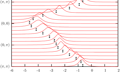
(b) $J_{\bot}/J_{\|}=2.4$

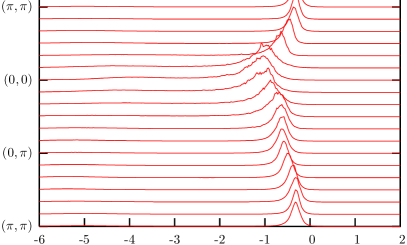
(c) $J_{\bot}/J_{\|}=2.0$

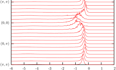
(d) $J_{\bot}/J_{\|}=1.0$
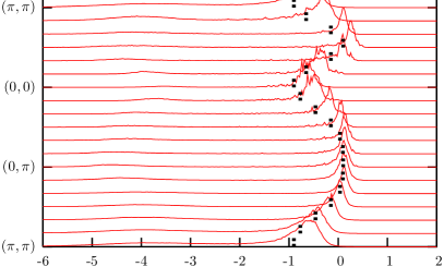
$\omega/J_{\|}$

Figure 5: Spectrums of a mobile hole for a $12\times 12$ lattice in the BHM. The small dashed lines in (a) tag the dispersion of a free particle; in (d) they outline a dispersion of the form: $E({\boldsymbol{p}})=J_{\|}\left(\cos(p)_{x}+\cos(p_{y})\right)^{2}$.

With decreasing coupling ratio the bandwidth of the quasiparticle dispersion relation diminishes but the overall features of the strong coupling remain.

In the weak coupling limit we observe considerable differences between the single particle spectrum of the BHM and KNM. Let us start with the BHM. For this model the point $J_{\bot}/J_{\|}=0$ is well defined (i.e. the ground is non-degenerate on any finite lattice) and corresponds to two independent Heisenberg planes with mobile hole in the upper plane. The problem of the single hole in a two dimensional Heisenberg model has been addressed in the framework of the self-consistent Born approximation Martinez91 , and yields a dispersion relation given by:

$$E({\boldsymbol{p}})=J_{\|}\left(\cos(p)_{x}+\cos(p_{y})\right)^{2}\,\,.$$ (36)

Since at $J_{\bot}/J_{\|}=0$ we have a well defined ground state we can expect that turning on a small value of $J_{\bot}/J_{\|}$ will not alter the single hole dispersion relation. This point of view is confirmed in Fig. 5. At $J_{\bot}/J_{\|}=1$, the single hole dispersion relation follows of Eq. (36). Hence and as confirmed by Fig. 5 the dispersion relation of a single hole in the BHM continuously deforms from the strong coupling form of Eq. (35) to that of a doped hole in a planar antiferromagnet (see Eq. (36)). Hence as a function of $J_{\bot}/J_{\|}$ there is a point where the effective mass (as defined by the inverse curvature of the dispersion relation) at ${\boldsymbol{p}}=(\pi,\pi)$ diverges. Upon inspection of the data (see Fig. 5), the point of divergence of the effective mass is not related to the magnetic quantum phase transition and since it occurs slightly below $\left(J_{\bot}/J_{\|}\right)_{c}$. This crossover between a dispersion with minimum at ${\boldsymbol{p}}=(\pi,\pi)$ and minimum at ${\boldsymbol{p}}=(\pi/2,\pi/2)$ with a crossover point lying inside the AF ordered phase is also documented in Ref. Vojta99 .

The above argument can not be applied to the KNM, since the $J_{\bot}/J_{\|}=0$ point is macroscopically degenerate and hence is not a good starting point to understand the weak-coupling physics. Clearly the same holds for the KLM and UKLM. Inspection of the spectral data deep in the ordered phase of the KNM (see Fig. 6c) shows that the maximum of the dispersion relation is still pinned at ${\boldsymbol{p}}=(\pi,\pi)$ such that the strong coupling features stemming from Kondo screening is still present at weak couplings. For the KNM and up to the lowest couplings we have considered the effective mass at ${\boldsymbol{p}}=(\pi,\pi)$ increases as a function of decreasing coupling strength but does not seem to diverge at finite values of $J_{\bot}/J_{\|}$. Precisely the same conclusion is reached in the framework of the KLM Capponi00 and UKLM Feldbacher02 .

(a) $J_{\bot}/J_{\|}=4.0$

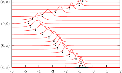
(b) $J_{\bot}/J_{\|}=2.0$

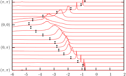
(c) $J_{\bot}/J_{\|}=0.5$
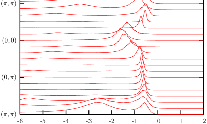
$\omega/J_{\|}$

Figure 6: Spectrum of the KNM for a $12\times 12$ lattice. The dashed lines tag the dispersion of a free particle.

IV Quasi Particle Residue

In this section we turn out attention to the delicate issue of the quasiparticle residue in the vicinity of the magnetic quantum phase transition. We first address this question within the framework of the the mean-field model of Eq. (III.2) and compute the single particle Green’s function within the framework of the self-consistent Born approximation. In a second step, we attempt to determine the quasiparticle residue directly from the Monte Carlo data.

IV.1 Analytical Approach

Here we restrict our analysis to the BHM. and return to the Hamiltonian (III.2). The coupling between the hole and magnons $g({\boldsymbol{p}},{\boldsymbol{q}})$ reads:

$$\quad g({\boldsymbol{p}},{\boldsymbol{q}})=g_{a}({\boldsymbol{p}},{\boldsymbol{q}})+g_{b}({\boldsymbol{p}},{\boldsymbol{q}}).$$

We identify the two coupling constants with the processes that are shown in Fig. 7: $g_{a}({\boldsymbol{p}},{\boldsymbol{q}})$ is proportional to the hopping matrix element and hence describes the coupling of a mobile hole to magnetic background, whereas $g_{b}({\boldsymbol{p}},{\boldsymbol{q}})$ is proportional to $J^{(2)}_{\|}$ and describes the coupling of a hole at rest with the magnons. Our calculations give the following momentum dependent coupling strengths:

$$g_{a}({\boldsymbol{p}},{\boldsymbol{q}}) = -\frac{t\bar{s}}{\sqrt{N}}\big{(}\gamma({\boldsymbol{p}}+{\boldsymbol{q}})u({\boldsymbol{q}})+\gamma({\boldsymbol{p}})v({\boldsymbol{q}})\big{)}$$ (37)

$$g_{b}({\boldsymbol{p}},{\boldsymbol{q}}) = -\frac{J^{(2)}_{\|}\bar{s}}{8\sqrt{N}}\gamma({\boldsymbol{q}})\big{(}u({\boldsymbol{q}})+v({\boldsymbol{q}})\big{)}$$ (38)

where $\gamma({\boldsymbol{q}})=2\big{(}\cos(q_{x})+\cos(q_{y})\big{)}$. We concentrate on the coupling to critical magnetic fluctuations and hence set ${\boldsymbol{q}}={\boldsymbol{Q}}$ and place ourselves in the proximity of the quantum phase transition, on the disordered side. In this case $\Omega({\boldsymbol{Q}})\rightarrow 0$ and the coherence factors (see Eq. (30)) are both proportional to $\Omega({\boldsymbol{q}})^{-\frac{1}{2}}$. Since furthermore $\gamma({\boldsymbol{p}}+{\boldsymbol{Q}})=-\gamma({\boldsymbol{p}})$ one arrives at the conclusion that $g_{a}({\boldsymbol{p}},{\boldsymbol{Q}})$ vanishes at the critical point.

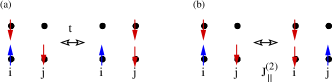
Figure 7: Two possible processes where the hole can couple to magnons: (a) The hole moves to a next neighbor. (b) The hole is at rest.

There is hence no coupling via process (a) to critical fluctuations. In other words process (a) couples only to short range spin fluctuations. On the other hand in the vicinity of the critical point $g_{b}$ scales as $g_{b}({\boldsymbol{p}},{\boldsymbol{q}})\propto\Omega({\boldsymbol{q}})^{-\frac{1}{2}}$ so that we can only retain this term to understand the coupling to critical fluctuations. Summarizing we set:

$$g({\boldsymbol{p}},{\boldsymbol{q}})\to g_{b}(\boldsymbol{q})\propto\frac{1}{\sqrt{\Omega(\boldsymbol{q})}}\,\,,$$ (39)

for the subsequent calculations. It is intriguing to note that in this simple approximation $g_{b}(\boldsymbol{q})$ scales as $J^{(2)}_{\|}$, which is strictly speaking null in the KNM. However, such a coupling should be dynamically generated via an RKKY-type interaction.

With the above couple the first order self energy diagram for wave vectors satisfying $\epsilon({\boldsymbol{p}})=\epsilon({\boldsymbol{p}}+{\boldsymbol{Q}})$ shows a logarithmic divergence as a function of the spin gap. Hence we have to sum up all diagrams. We do so in the non-crossing or self-consistent Born approximation which in the $T=0$ limit boils down to the following set of self-consistent equations.

$$\Sigma({\boldsymbol{p}},\omega) = \frac{1}{N}\sum_{{\boldsymbol{q}}}g^{2}({\boldsymbol{p}},{\boldsymbol{q}})G({\boldsymbol{p}}-{\boldsymbol{q}},\omega-\Omega({\boldsymbol{q}}))$$

$$G({\boldsymbol{p}},\omega) = \frac{1}{\omega-\varepsilon({\boldsymbol{p}})-\Sigma({\boldsymbol{p}},\omega)}$$ (40)

Here we use a magnon dispersion relation of the form $\Omega({\boldsymbol{q}})=\sqrt{\Delta^{2}+v^{2}_{s}\left(1+\gamma({\boldsymbol{q}})/4\right)}$ with $\gamma({\boldsymbol{q}})=2\big{(}\cos(q_{x})+\cos(q_{y})\big{)}$, which agrees in the limit ${\boldsymbol{q}}\to{\boldsymbol{Q}}=(\pi,\pi)$ with the form of Eq. (31). Iterating the Green’s function up to the 15th order to ensure convergence, we calculate the spectrum, $\rho({\boldsymbol{p}},\omega)=\frac{1}{\pi}Im[G({\boldsymbol{p}},\omega)]$ via the imaginary part of the Green’s function and compute the quasi-particle residue (QPR) at the first pole of the spectrum.

$$\mathcal{Z}({\boldsymbol{p}})=\Big{|}1-\frac{\partial}{\partial\omega}\Sigma^{\prime}({\boldsymbol{p}},\omega)\Big{|}^{-1}_{\omega=\omega_{i}}$$ (41)

Figure 8 shows the QPR for ${\boldsymbol{p}}=(\pi,\pi)$ as a function of linear length $L$ of the square lattice for different values of the spin gap $\Delta$. The large-$L$ limit is indicated by a line.

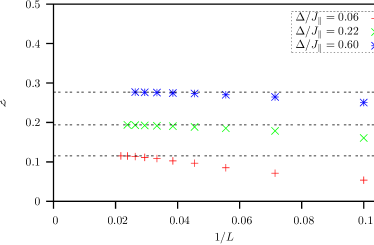
Figure 8: Self consistent Born approximation: QPR as a function of linear lattice size, $L$, for different spin gap energies, $\Delta$.

Figure 9 plots the quasiparticle weight as a function of the spin gap for hole momenta ${\boldsymbol{p}}=(\frac{\pi}{2},\frac{\pi}{2}),(0,\pi),(\pi,\pi)$.

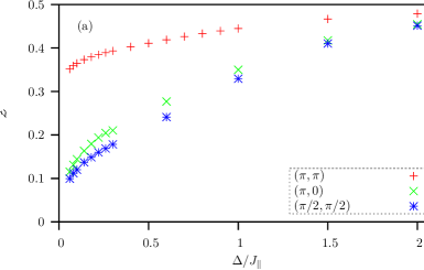
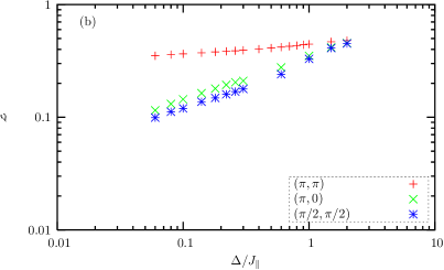
Figure 9: Self consistent Born approximation: QPR in the vicinity of the quantum critical point for selected hole momenta (a) in a linear plot and (b) in a double logarithmic plot. $\Delta$ corresponds to the spin gap.

For hole momenta satisfying $\epsilon({\boldsymbol{p}})=\epsilon({\boldsymbol{p}}+{\boldsymbol{Q}})$ ( ${\boldsymbol{p}}=(\frac{\pi}{2},\frac{\pi}{2})$ and ${\boldsymbol{p}}=(0,\pi)$ ) there is no energy denominator prohibiting the logarithmic divergence of the first order self-energy and the QPR shows an obvious decrease right up to a complete vanishing at the critical point. Furthermore, the data is consistent with $\mathcal{Z}\propto\sqrt{\Delta}$. The case ${\boldsymbol{p}}=(\pi,\pi)$ is more complicated since $\epsilon({\boldsymbol{p}})\neq\epsilon({\boldsymbol{p}}+{\boldsymbol{Q}})$. In first order, the self-energy remains bounded. The scattering of the hole of ${\boldsymbol{Q}}=(\pi,\pi)$ magnons leads to the progessive formation of shadow bands as the critical point is approached such that at the critical point, the relation $E^{(1)}({\boldsymbol{p}})=E^{(1)}({\boldsymbol{p}}+{\boldsymbol{Q}})$ holds. This back folding of the band can lead to the vanishing of the QPR when higher order terms are included. Although the SCB results show a decrease of the QPR in the vicinity of the critical point, they are not accurate enough to answer the question of the vanishing of the QPR at this wave vector.

IV.2 QMC approach

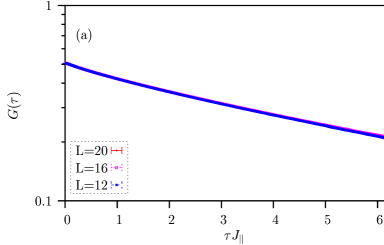
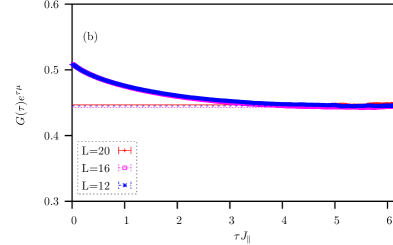
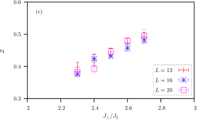
Figure 10: Green’s function in the vicinity of the phase transition ($J_{\bot}/J_{\|}=2.5$) for a static hole and various lattice sizes in the BHM (a) on a logarithmic plot and (b) on a plot where we adjusted the chemical potential in such a way that the Green’s function converges to a constant value. Within the error bars and for lattice sizes greater then $12\times 12$ there is no size scaling recognisable. (Inverse temperatures: $\beta J_{\|}=30$ ($L=12$), $\beta J_{\|}=50$ ($L=16$)), $\beta J_{\|}=70$ ($L=20$); $\Delta\tau J_{\|}=0.02$) (c) QPR in the vicinity of the quantum critical point.

As shown in section II we can extract the QPR from the asymptotic behavior of the Green’s function. We first concentrate on the static hole in the BHM for which the QMC data is of higher quality that for the dynamic hole. Fig. 10a plots the Green’s funtion as a function of lattice size at $J_{\bot}/J_{\|}=2.5$. As apparent within the considered range of imaginary times no size and temperature effect is apparent. We fit the tail ( $5<\tau J_{\|}<6$) of the Green’s function to the form $\mathcal{Z}e^{-\tau\mu}$ and plot in Fig. 10b $G(\tau)e^{\tau\mu}$. In the large imgaginary time limit this quantitiy converges to the QPR $\mathcal{Z}$. The so obtained value of $\mathcal{Z}$ is plotted for values of $J_{\bot}/J_{\|}$ across the magnetic quantum phase transition. As apparent no sign of the vanishing of the QPR is apparent as we cross the quantum critcal point.

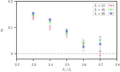
Figure 11: $\eta_{h}$ (see Eq. (42)) as a function of $J_{\bot}/J_{\|}$ for a static hole in the BHM.

Our QMC data allows a different interpretation. Following the work of Sachdev et al. Sachdev01 we fit the imaginary time Green function to the form:

$$G(\tau)\propto\tau^{-\eta_{h}}\exp\left(-\tau\mu\right)$$ (42)

in the the range $2.0<\tau J_{\|}<6.0$ as done in Ref. Sachdev01 . Clearly, if $\eta_{h}>0$ then the QPR vanishes. Our results for $\eta_{h}$ are plotted in Fig. 11. At $J_{\bot}/J_{\|}=2.5$ our result, $\eta_{h}=0.0875\pm 0.0085$ compares very well to that quoted in Ref. Sachdev01 , $\eta_{h}=0.087\pm 0.040$. The fact that the result of Ref. Sachdev01 is obtained on a $64\times 64$ lattice and ours on $20\times 20$ confirms that for the considered imaginary time range, size effects are absent. Given the above interpretation of the data, Fig. 11 suggests that QPR of a static hole vanishes for all $J_{\bot}/J_{\|}\leq\left(J_{\bot}/J_{\|}\right)_{c}\simeq 2.5$.

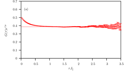
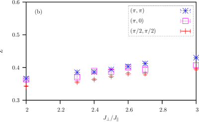
Figure 12: Green’s function of a dynamic hole (${\boldsymbol{p}}=(\pi,\pi)$) in the BHM for a $12\times 12$ lattice at $J_{\bot}/J_{\|}=2.4$. (b) QPR in the vicinity of the quantum critical point.

The choice of the fitting function reflects different ordering of the limits $\tau\rightarrow\infty$ and $N\rightarrow\infty$. On any finite size lattice the QPR is finite and hence it is appropriate to fit the tail of the Green’s function to the form $\mathcal{Z}(N)e^{-\tau\mu}$ to obtain a size dependend QPR, and subsequently take the thermodynamic limit. This strategy has been used successfully to show that the QPR of a doped mobile hole in a one dimensional Heisenberg chain vanishes Brunner00 . On the other hand, the choice of Eq. (42) for fitting the data implies that we first take the thermodynamic limit. Only in this limit, can the assymptotic form of the Green’s function follow Eq. (42) with $\eta_{h}\neq 0$. The fact that both procedures yield different results sheds doubt on the small imaginary time range used to extract the quasiparticle residue. In particular, using data from $\tau J_{\|}=2$ onwards implies that we are looking at a frequency window around the lowest excitation of the order $\omega/J\simeq 0.5$. Given this, it is hard to resolve the difference between a dense spectrum and a well defined low-lying quasiparticle pole and a branch cut.

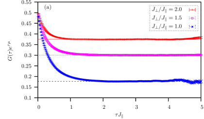
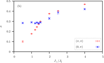
Figure 13: (a) Green’s function $G_{\boldsymbol{p}}(\tau)$ in the Kondo Necklace model at ${\boldsymbol{p}}=(\pi,\pi)$ for $J_{\bot}/J_{\|}=1.0,1.5,2.0$. (b) Extracted values for the QPR. The critical point is localised at $(J_{\bot}/J_{\|})_{c}=1.360\pm 0.017$.

We conclude this section by presenting data for a mobile hole in the BHM (see Fig. 12) and KNM (see Fig. 13). Recall that in our simulations we restrict the motion of the hole to a single plane. The data for the QPR in the above mentioned figures stem from fitting the tail of the Green’s function to the form $\mathcal{Z}e^{-\tau\mu}$. The fit to the form of Eq. (42) yields values of $\eta_{h}$ which within the error bars are not distinguishable form zero.

V Conclusion

We have analyzed single hole dynamics across magnetic order-disorder quantum phase transitions as realized in the Kondo Necklace and bilayer Heisenberg models. The hole motion is restricted to the upper layer as appropriate for interpretation of the data in terms in Kondo physics. Both models have identical spin dynamics since the quantum phase transition is described by the $O(3)$ three-dimensional sigma model Troyer97 . On the other hand the single hole dynamics shows marked differences. In the strong coupling limit, deep in the disordered phase, the ground state of both models is well described by a direct product of singlets between the layers. This Kondo screening leads to a single hole dispersion relation with maximum at ${\boldsymbol{p}}=(\pi,\pi)$. In the Kondo Necklace model, where the spin degrees of freedom on the lower layer interact indirectly through polarization of spin on the upper layer (RKKY type interaction), the single hole dispersion preserves it’s maximum at $\boldsymbol{p}=(\pi,\pi)$ down to arbitrarily low interplanar couplings. This situation is very similar to the Kondo Lattice model of Eq. (1). In this case, down to $\mathcal{J}/t=0.2$, substantially below the magnetic phase transition $\mathcal{J}_{c}/t=1.45\pm 0.05$, the maximum of the the hole dispersion is pinned at $\boldsymbol{p}=(\pi,\pi)$ and the effective mass at this ${\boldsymbol{p}}$-point tracks the single ion Kondo temperature Assaad04a . We note that this result is not supported by recent series expansions which show that there is a critical value of the coupling where the effective mass diverges Trebst06 . Hence the interpretation that in both the Kondo necklace and Kondo lattice models, the localized spins remained partially screen down to arbitrarily low values of the interlayer coupling. In other words, signatures of strong coupling physics in the single hole dispersion relation is present down to arbitrary low interplanar couplings.

In the bilayer Heisenberg model where there is an independent energy scale coupling the spins on the lower layer, the situation differs. At values of $J_{\bot}<J_{\bot,c}$ the maximum of the single hole dispersion relation drifts towards ${\boldsymbol{p}}=(\pi/2,\pi/2)$ and the dispersion relation evolves continuously to that of a single hole doped in a planar antiferromagnetic Brunner00b . Hence the interpretation that at weak couplings, Kondo screening in this model is completely suppressed. In other words, the small but finite $J_{\bot}$ results can be well understood starting form the $J_{\bot}=0$ point.

We have equally, analyzed the quasiparticle residue across the magnetic order-disorder transition. In the disordered phase using a bond mean-field approximation, there are two processes in which the hole couples to magnetic fluctuations (see Fig. 7): i) The hole propagates from one lattice site to another thereby rearranging the spin background. In the proximity of the critical point, and still within the bond-mean field approximation those processes do not couple to long range $\boldsymbol{Q}=(\pi,\pi)$ magnetic fluctuations. A very similar result is obtained in the ordered phase Martinez91 . ii) In bilayer models the hole can remain immobile and the spin in the lower layer can flip. Those processes couple to critical magnetic fluctuations. Within a self-consistent Born approximation, this drives the quasiparticle residue to zero both for a static hole and mobile hole with momenta ${\boldsymbol{p}}$ satisfying $\epsilon({\boldsymbol{p}}+{\boldsymbol{Q}})=\epsilon({\boldsymbol{p}})$. We have attempted to confirm this point of view with Monte Carlo simulations. Within our quantum Monte Carlo approach, where the accuracy of the single particle Green’s function at large imaginary times is limited, we have found no convincing evidence of the vanishing of the quasiparticle residue both for a static and a mobile hole. Furhter work and algortihmic developments are required to clarify this delicate issue.

Acknowledgments. The calculations were carried out on the Hitachi SR8000 of the LRZ München. We thank this institution for generous allocation of CPU time. We have greatly profitted from discussions with M. Vojta and L. Martin. Financial support from the DFG under the grant number AS120/4-1 is acknowledged.

References

- (1) S. Paschen, T. Lühmann, S. Wirth, P. Gegenwart, O. Trovarelli, C. Geibel, F. Steglich, P. Coleman, and Q. Si, Nature 432, 881 (2004).
- (2) J. R. Schrieffer and P. A. Wolff, Phys. Rev. 149, 491 (1966).
- (3) H. Tsunetsugu, M. Sigrist, and K. Ueda, Rev. Mod. Phys. 69, 809 (1997).
- (4) S. Capponi and F. F. Assaad, Phs. Rev. B 63, 155114 (2001).
- (5) M. Feldbacher, C. Jurecka, F. F. Assaad, and W. Brenig, Phys. Rev. B 66, 045103 (2002).
- (6) M. Brunner, F. F. Assaad, and A. Muramatsu, Eur. Phys. J. B 16, 209 (2000).
- (7) K. S. D. Beach, cond-mat/0403055 (2004).
- (8) A. Sandvik, Phys. Rev. B 57, 10287 (1998).
- (9) O. P. Sushkov, Phys. Rev. B 62, 12135 (2000).
- (10) H. G. Evertz, Adv. Phys. 52, 1 (1997).
- (11) A. Angelucci, Phys. Rev. B 51, 11580 (1995).
- (12) M. Troyer, M. Imada, and K. Ueda, J. Phys. Soc. Jpn. 66, 2957 (1997).
- (13) P. V. Shevchenko, A. W. Sandvik, and O. P. Sushkov, Phys. Rev. B 61, 3475 (2000).
- (14) V. N. Kotov, O. Sushkov, Z. Weihong, and J. Oitmaa, Phys. Rev. Lett. 80, 5790 (1998).
- (15) S. Sachdev and R. N. Bhatt, Phys. Rev. B 41, 9323 (1990).
- (16) M. Vojta and K. W. Becker, Phys. Rev. B 60, 15201 (1999).
- (17) G. Martínez and P. Horsch, Phys. Rev. B 44, 317 (1991).
- (18) S. Sachdev, M. Troyer, and M. Vojta, Phys. Rev. Lett. 86, 2617 (2001).
- (19) F. F. Assaad, Phys. Rev. B 70, 020402 (2004).
- (20) S. Trebst, H. Monien, A. Grzesik, and M. Sigrist, Phys. Rev. B 73, 165101 (2006).
- (21) M. Brunner, F. F. Assaad, and A. Muramatsu, Phys. Rev. B 62, 12395 (2000).