Statics and dynamics of BEC’s in double square well potentials.

Abstract

In this paper we treat the behavior of Bose Einstein condensates in double square well potentials, both of equal and different depths. For even depth, symmetry preserving solutions to the relevant nonlinear Schrödinger equation is known, just as in the linear limit. When the nonlinearity is strong enough, symmetry breaking solutions also exist, side by side with the symmetric one. Interestingly, solutions almost entirely localized in one of the wells are known as an extreme case. Here we outline a method for obtaining all these solutions for repulsive interactions. The bifurcation point at which, for critical nonlinearity, the asymmetric solutions branch off from the symmetry preserving ones is found analytically. We also find this bifurcation point and treat the solutions generally via a Josephson Junction model.

When the confining potential is in the form of two wells of different depth, interesting new phenomena appear. This is true of both the occurrence of the bifurcation point for the static solutions, and also of the dynamics of phase and amplitude varying solutions. Again a generalization of the Josephson model proves useful. The stability of solutions is treated briefly.

I Introduction

The nonlinear Schrödinger equation is a powerful tool for describing Bose Einstein condensates at zero temperature. Double well potentials are an important class of configurations to which this tool can be applied. For square wells, exact solutions are known to exist Reinhardt . In Ziń et al. Zin , we outlined a method for obtaining such exact solutions for a symmetric double square well situation with attractive interaction. We found an exact criterion to determine the bifurcation point. Here we perform similar calculations for the repulsive case and extend our treatment, including wells of different depth but also a stability analysis. The repulsive case is perhaps more interesting in view of the fact that, for this interaction, situations such that most of the condensate was contained in one of the wells have been seen experimentally Oberthaler . We also present some dynamic calculations not included in Zin for both kinds of interaction. These lean somewhat on a generalized Josephson Junction model Adams ; elena ; Giovanazzi ; Smerzi ; Raghavan . We note in passing that a Josephson Junction for a Bose-Einstein condensate was first obtained by Inguscio’s group JosBEC , see also Oberthaler .

Symmetry breaking solutions that are known to exist for positive nonlinearity (repulsive interaction in the case of BEC, dark solitons in nonlinear optical media) often tend to localize the wave function in one of the wells. This happens for the nonlinearity exceeding a critical value at which the asymmetric solutions branch off from the symmetry preserving ones in the parameter space. Therefore, we can talk about bifurcation at this critical value of nonlinearity. The existence of such solutions of the nonlinear Schrödinger equation was first pointed out in the context of molecular states for repulsive interaction Davis , as will be treated here. Importantly, the effect of this spontaneous symmetry breaking has been observed in photonic lattices kevrekidis . It should be stressed that the nature of bifurcation depends on the symmetry of the problem and is of the pitchfork variety for even wells and saddle point for uneven wells Ioos .

In this paper we will consider a double square well potential, first symmetric and then asymmetric. The asymmetric potential leads to more complicated profiles. As far as we know, these square well configurations are the only ones for which exact solutions exist. These solutions are all in the form of Jacobi elliptic functions. One of the problems considered here, extending Zin to repulsive interaction, is how to proceed from easily obtainable symmetric double well solutions of the linear Schrödinger equation to the fully nonlinear case, and from so obtained symmetric solutions on to the bifurcated, asymmetric ones. When the potential is asymmetric both bifurcation of the static solutions and the dynamics of oscillating solutions will be seen to become very different from those for the symmetric potential.

The manuscript is composed as follows: In section II we derive symmetry preserving states starting from the linear limit and then gradually increasing the nonlinear interaction. In section III we investigate the symmetry breaking states that branch off from the symmetry preserving ones in the parameter space. We give a simple exact formula for the bifurcation point. Section IV treats asymmetric potentials. Section V is devoted to dynamics treated by the Josephson model, particularly useful at the bifurcation point, and then numerically. Results are consistent by all three methods (sections III, IV and V). Some concluding remarks wind up the text (section VI). Heavier calculations have been relegated to the Appendix.

This paper can be read independently of reference Zin .

II Antisymmetric states from the linear limit (symmetric wells)

We start from the nonlinear Schrödinger equation

$$\left[-\frac{\partial^{2}}{\partial x^{2}}+V(x)+\eta|f(x)|^{2}\right]f(x)=\mu f(x)$$ (1)

Here the potential is of the form

$$V(x)=\left\{\begin{array}[]{lll}V_{0}&\mbox{ for }|x|\leq b\\ 0&\mbox{ for }b<|x|\leq a\\ \infty&\mbox{ for }|x|\geq a\end{array}\right.$$ (2)

See Fig. 1. Solutions in the three regions will be written as

$$f(x)=\left\{\begin{array}[]{lll}f_{1}(x)&\mbox{ for }-a\leq x<-b\\ f_{2}(x)&\mbox{ for }|x|\leq b\\ f_{3}(x)&\mbox{ for }b<x\leq a\end{array}\right.$$ (3)

The solutions vanish on and outside the outer boundaries $|x|\geq a$. We assume continuity of $f(x)$ and its derivative at $x=\pm b$ and normalization to $\int^{a}_{-a}|f(x)|^{2}\,dx=1$. The symmetric solutions are

$$f_{1}(x) = A\,\,\mbox{sn}(k(x+a)|m)$$ (4)

$$f_{2}(x) = A_{2}\,\,\mbox{nc}(k_{2}x|m_{2})$$

$$f_{3}(x) = -A\,\,\mbox{sn}(k(x-a)|m)$$

and the antisymmetric solutions, which will be of particular interest here, are

$$f_{1}(x) = A\,\,\mbox{sn}(k(x+a)|m)$$ (5)

$$f_{2}(x) = -A_{2}\,\,\mbox{sc}(k_{2}x|m_{2})$$

$$f_{3}(x) = A\,\,\mbox{sn}(k(x-a)|m).$$

Here $f_{1}(x)$ and $f_{3}(x)$ have been chosen to be zero at the ends, and also so as to preserve even and odd parity respectively for the two cases. The parameters of the symmetric solutions are found from Eq. (1) to satisfy ($V_{0}>\mu$)

$$A^{2}=\frac{2mk^{2}}{\eta},\ \ \ \ \ \ A_{2}^{2}=\frac{2(1-m_{2})k_{2}^{2}}{\eta},\ \ \ \ \ \ \mu=(1+m)k^{2}=(1-2m_{2})k_{2}^{2}+V_{0},$$ (6)

and for the antisymmetric solutions we have

$$A^{2}=\frac{2mk^{2}}{\eta},\ \ \ \ \ \ A_{2}^{2}=\frac{2(1-m_{2})k_{2}^{2}}{\eta},\ \ \ \ \ \ \mu=(1+m)k^{2}=(m_{2}-2)k_{2}^{2}+V_{0}.$$ (7)

Positive roots for all the A’s are taken throughout. We choose $\mu$, $m$ and $m_{2}$ to generate all the other constants. These three parameters will determine the solution completely.

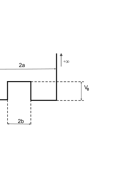
Figure 1: Symmetric double square well potential. In the following $2a=1$, $2b=0.1$ and $V_{0}=300$.

We now concentrate on the antisymmetric case, as we have checked that bifurcation only occurs for this case in the lowest mode as suggested by Fig. 4 (and also by Fig. 3 of Ref. Dagosta ). We have two continuity conditions at $\pm b$

$$A\mbox{sn}(k\omega|m)=-A_{2}\mbox{sc}(-k_{2}b|m_{2})$$ (8)

$$Ak\mbox{cn}(k\omega|m)\mbox{dn}(k\omega|m)=-A_{2}k_{2}\mbox{dc}(-k_{2}b|m_{2})\mbox{nc}(-k_{2}b|m_{2}).$$ (9)

Here $\omega=a-b$. The normalization of the wave function, $\int_{-a}^{a}\mbox{d}x\,|f(x)|^{2}=1$ yields

$$2A^{2}\int_{a}^{b}\mbox{sn}^{2}(k(x-a)|m)\mbox{d}x+2A_{2}^{2}\int_{0}^{b}\mbox{sc}^{2}(k_{2}x|m_{2})\mbox{d}x=1$$

The above normalization condition works out as:

$${4k_{2}}\left[\mbox{sn}(k_{2}b|m_{2})\ \mbox{dc}(k_{2}b|m_{2})-E(k_{2}b|m_{2})\right]+{4k}\left[k\omega-E(k\omega|m)\right]={\eta},$$ (10)

where $E(u|m)$ is the elliptic function of the second kind Abram . We now have three equations for $m$, $m_{2}$ and $\mu$ as required. Here $a$, $b$, $V_{0}$ and $\eta$ are fixed and describe one specific experimental setup. Up to now, the shooting method was used to find solutions Reinhardt .

To systematically solve our equations we first turn to the linear limit $\eta=0$, $k^{2}=\mu$, $k_{2}^{2}=V_{0}-\mu$. The functions are now easy to calculate

$$f_{1}(x) = A\,\,\sin k(x+a)$$

$$f_{2}(x) = -A_{2}\,\,\sinh k_{2}x$$

$$f_{3}(x) = A\,\,\sin k(x-a).$$

The two continuity conditions are:

$$A\,\,\sin k\omega = A_{2}\sinh k_{2}b$$ (11)

$$Ak\,\,\cos k\omega = -A_{2}k_{2}\,\,\cosh k_{2}b,,$$ (12)

This last equation will give us linear $\mu$ in terms of fixed parameters. The normalization condition is

$$A^{2}=\left(\omega-\frac{\sin 2k\omega}{2k}+\frac{\sin^{2}k\omega}{\sinh^{2}k_{2}b}\left(-b+\frac{\sinh 2k_{2}b}{2k_{2}}\right)\right)^{-1}.$$ (13)

Giving a value for $A$, and $A_{2}$ follows from continuity. We are now ready to tie this solution up to the small $\eta$ limit in a perturbative manner. We notice that $A,A_{2},k,k_{2}$ obtained in the linear approach become a zero order approximation in an $\eta$ expansion. The parameters $m$ and $1-m_{2}$ are both of order $\eta$ and follow from equations (6) and (11)

$$m=\frac{A^{2}}{2k^{2}}\eta\ \ \ \ 1-m_{2}=\frac{\sin^{2}k\omega}{\sinh^{2}k_{2}b}\frac{A^{2}}{2k_{2}^{2}}\eta.$$ (14)

Linear $\mu$, denoted by $\mu_{0}$, is found as the lowest root of

$$\sqrt{\mu_{0}}\cot(\sqrt{\mu_{0}}\omega)+\sqrt{V_{0}-\mu_{0}}\coth(\sqrt{V_{0}-\mu_{0}}b)=0.$$ (15)

There will also be a small $\eta$ correction $\Delta\mu$ such that $\mu=\mu_{0}+\Delta\mu$. This will complete the calculation of the three unknowns $\mu$, $m$, $m_{2}$ in the small $\eta$ limit (Appendix).

Now that we have a starting point, we can generate all symmetric solutions by gradually increasing $\eta$. We introduce the notation $\mu\equiv m_{0},\,\,\,m\equiv m_{1}$, and $m_{2}$. We write the conditions (8) and (9) in the symbolic functional form

$$h_{0}(m_{0},m_{1},m_{2})=k\sqrt{m_{1}}\,\,\mbox{sn}(k\omega|m_{1})-k_{2}\sqrt{(1-m_{2})}\,\,\mbox{sc}(k_{2}b|m_{2})=0,$$ (16)

$$h_{1}(m_{0},m_{1},m_{2})=k^{2}\sqrt{m_{1}}\,\,\mbox{cn}(k\omega|m_{1})\,\,\mbox{dn}(k\omega|m_{1})+k_{2}^{2}\sqrt{1-m_{2}}\,\,\mbox{dc}(k_{2}b|m_{2})\,\,\mbox{nc}(k_{2}b|m_{2})=0.$$ (17)

Here we used Eq. (6) to express the amplitudes $A$ and $A_{2}$ in terms of the $m_{i}$ and the wavevectors $k$ and $k_{2}$, which in turn can be expressed in terms of the $m_{i}$. The left hand side of equation (10) defines $h_{2}(m_{0},m_{1},m_{2})$, which is evidently free of $\eta$. Upon defining $\eta_{0}=0,\,\eta_{1}=0,\,\eta_{2}=\eta$ we write all three conditions (8), (9) and (10) simply as

$$h_{i}(m_{0},m_{1},m_{2})=\eta_{i}\ \ \ \mbox{for}\ \ \ i=0,1,2.$$ (18)

In all three equations (18) functions $h_{i}(m_{0},m_{1},m_{2})$ on the left, remain free of $\eta$. Hence if we increase $\eta$ by a small increment $\Delta\eta$ the parameters $m_{i}$ will increase by $\Delta m_{i}$ governed by

$$\left(\frac{\partial h_{i}}{\partial m_{j}}\right)\Delta m_{j}=\Delta\eta_{i},$$ (19)

where $\Delta\eta_{i}=(0,0,\Delta\eta)$. Assuming the matrix $\left(\frac{\partial h_{i}}{\partial m_{j}}\right)$ to be nonsingular we can now generate increments in $m_{i}$ by gradually increasing the control parameter $\eta$. Inverting Eq. (19) we find

$$\Delta m_{i}=\left(\frac{\partial h_{i}}{\partial m_{j}}\right)^{-1}\Delta\eta_{j}.$$ (20)

III Symmetry Breaking States (symmetric wells)

Even when the double well is symmetric, the nonlinear Schrödinger equation is known to admit symmetry breaking states. This is in contradistinction to the linear version, admitting only symmetric and antisymmetric states as treated in section (II). These symmetry breaking states are possible above a critical value of $\eta$. They are of considerable physical interest, as they include situations such as the location of most of the wavefunction in one half of the double well. More generally, there is the possibility of very different profiles in the two halves. The solutions corresponding to symmetry breaking are known to bifurcate from the antisymmetric ones. Here we will give a condition defining the bifurcation points in parameter space and investigate how this bifurcation can be interpreted. We will give diagrams to illustrate this. Similar diagrams for a quartic potential can be found in Dagosta , however they do not correspond to any analytic solutions known to us.

Solutions generalizing the symmetric case are:

$$f_{1}(x) = A_{1}\,\,\mbox{sn}(k_{1}(x+a)|m_{1})$$

$$f_{2}(x) = A_{2}\,\,\mbox{nc}(k_{2}(x+d)|m_{2})$$

$$f_{3}(x) = -A_{3}\,\,\mbox{sn}(k_{3}(x-a)|m_{3})$$

and the generalization for the antisymmetric case is:

$$f_{1}(x) = A_{1}\,\,\mbox{sn}(k_{1}(x+a)|m_{1})$$

$$f_{2}(x) = -A_{2}\,\,\mbox{sc}(k_{2}(x+d)|m_{2})$$

$$f_{3}(x) = A_{3}\,\,\mbox{sn}(k_{3}(x-a)|m_{3}).$$

When $d=0$, $m_{1}=m_{3}=m$ the solutions (4) and (5) are recovered. Once again we concentrate on a generalization of the antisymmetric case, as the only one branching off from a basic mode.

We now have five conditions for $\mu,m_{1},m_{2},m_{3},d$, which we will denote $m_{I}$    $I=0,...4$ and in place of equation (18) we have $g_{I}=\eta_{I}$, see the Appendix. One solution is $d=0,m_{1}=m_{2}=m$, as we know, and conditions (8), (9) and (10) are recovered. However, as we will see, above a certain threshold in $\eta$ a second solution appears. The value of $\eta$ at which this bifurcation occurs will be denoted by $\eta_{bif}$. The second solution branches off the antisymmetric one at this point. To find it we note that at such a point the antisymmetric solution is continuous with respect to $\eta$, whereas the asymmetric one is not. Therefore we expect the $3\times 3$ matrix $\left(\frac{\partial h_{i}}{\partial m_{j}}\right)$ to be nonsingular, whereas the $5\times 5$ matrix $\left(\frac{\partial g_{I}}{\partial m_{J}}\right)$ will be singular at this point. Simple algebra shows that the determinant of the $5\times 5$ matrix can be factorized at the bifurcation point for which $m_{1}=m_{3}$ and $d=0$.

$$\det\left(\frac{\partial g_{I}}{\partial m_{J}}\right)=\det\left(\frac{\partial h_{i}}{\partial m_{j}}\right)D_{2}$$ (21)

and $D_{2}$ is found to be given by:

$$D_{2}=2\left[\frac{\partial g_{0}}{\partial m_{1}}\frac{\partial g_{2}}{\partial d}-\frac{\partial g_{0}}{\partial d}\frac{\partial g_{2}}{\partial m_{1}}\right]_{m_{1}=m_{3},d=0}$$ (22)

In view of the above, $D_{2}=0$. This condition can be expressed in terms of variables characterizing the antisymmetric solution. If we write conditions (16), (17) as $h_{0}=h_{0}^{(1)}-h_{0}^{(2)}$ and $h_{1}=h_{1}^{(1)}+h_{1}^{(2)}$ we obtain a simple condition for the bifurcation point:

$$\partial_{b}h_{1}^{(2)}\partial_{m}h_{0}^{(1)}+\partial_{m}h_{1}^{(1)}\partial_{b}h_{0}^{(2)}=0.$$ (23)

This further simplifies to:

$$\frac{\partial}{\partial m}\left[mk^{4}-mk^{2}V_{0}\mbox{sn}^{2}(k\omega|m)\right]=0.$$ (24)

Figure 2: Antisymmetric and asymmetric solutions for the same value of $\eta=10$.

Thus we can find the bifurcation point on the antisymmetric branch in terms of just two of the antisymmetric variables. Having that point we can move out onto the asymmetric branch using:

$$\Delta m_{I}=\left(\frac{\partial g_{I}}{\partial m_{J}}\right)^{-1}\Delta\eta_{J},\ \ \ \ \ \ \eta_{I}=0\ \ \ \mbox{for}\ \ \ I=0,1,2,3\ \ \ \mbox{and}\ \ \ \eta_{4}=\eta.$$ (25)

This equation can be used everywhere except at the branch point, where second derivatives must come in. We have checked numerically that condition (24) is always satisfied at the bifurcation point. For an illustration of a bifurcated asymmetric solution paired with the corresponding symmetry preserving one far from bifurcation, see Fig. 2.

IV Asymmetric Potential

Suppose now that the right hand well is somewhat shallower that on the left ($V=V_{3},\,\,b<x<a,\,\,0<V_{3}<\mu$). Otherwise we keep the notation of Fig. 1. Eqn. (6) is now replaced by

$$A_{1}^{2}=\frac{2m_{1}k_{1}^{2}}{\eta},\ \ \ A_{2}^{2}=\frac{2(1-m_{2})k_{2}^{2}}{\eta},\ \ \ A_{3}^{2}=\frac{2m_{3}k_{3}^{2}}{\eta},\ \ \ \mu=(1+m_{1})k_{1}^{2}=(1-2m_{2})k_{2}^{2}+V_{0}=(1+m_{3})k_{3}^{2}+V_{3}.$$ (26)

Equation (7) is similarly modified. When this is done all formulas for the symmetry breaking case formally carry through, with the understanding that $k_{3}^{2}$ is now $(\mu-V_{3})/(1+m_{3})$. Interchanging $m_{1}$ and $m_{3}$ no longer gives a trivial alteration. Solutions with most of the condensate on the left or on the right are no longer mirror images. Also, the linear limit is altered, relevant equations becoming

$$f_{1}(x) = A_{1}\,\,\sin k_{1}(x+a)$$

$$f_{2}(x) = -A_{2}\,\,\sinh k_{2}(x+d)$$

$$f_{3}(x) = A_{3}\,\,\sin k_{3}(x-a).$$

Even in this limit, we now have five equations for five unknowns: $m_{1}$, $m_{2}$, $m_{3}$, $\mu$ and $d$. This limit is thus nolonger much simpler than the fully nonlinear case. However this is not worth pursuing, as the interesting bifurcation does not now occur from the ”linear” branch.

Illustrations of how phase diagrams are modified as compared to the symmetric potential case are given in Fig. 5, E and F. As we increase $\eta$ from zero, a new double fixed point suddenly appears and bifurcates as we increase $\eta$ (see the next section). Thus we have two new fixed points (nolonger a pitchfork bifurcation).

V A Josephson Junction approach

Now allow $f$ to be time dependent and satisfy the one dimensional equation

$$i\frac{\partial f(x,t)}{\partial t}=\left[-\frac{\partial^{2}}{\partial x^{2}}+V(x)+\eta|f(x,t)|^{2}\right]f(x,t),$$ (27)

with potential $V(x)$ in the form of a double well, which is not necessarily symmetric. To establish a link between the above equation and the Josephson model, we first focus on the energy spectrum of the system in the linear limit ($\eta=0$). It consists of pairs of energy levels separated by a gap that is proportional to the height of the barrier; for a sufficiently high barrier the spacing between the pairs is larger than the spacing within the first pair. In this case we can construct a variational analysis based on the lowest pair of levels, $\psi_{1}$ and $\psi_{2}$. We assume that $f(x,t)$ is normalized to unity and approximate it by $f(x,t)\simeq a_{L}(t)w_{L}(x)+a_{R}(t)w_{R}(x)$, where $w_{L,R}(x)$ are defined as

$$w_{L,R}(x)=\frac{1}{\sqrt{2}}(\psi_{1}(x)\mp\psi_{2}(x)).$$ (28)

The eigenstates $\psi_{1}(x)$ and $\psi_{2}(x)$ are orthonormal. Amplitudes $a_{L,R}$ must satisfy $|a_{L}|^{2}+|a_{R}|^{2}=1$ and their time derivatives are approximately given by

$$i\dot{a}_{L,R}(t)=E_{0}a_{L,R}(t)-Ka_{R,L}(t)+U_{L,R}|a_{L,R}(t)|^{2}a_{L,R}(t),$$ (29)

where

$$E_{0}=\int w_{L,R}^{*}(x)\left[-\frac{\partial^{2}}{\partial x^{2}}+V(x)\right]w_{L,R}(x),\,\,\,K=-\int w_{L}^{*}(x)\left[-\frac{\partial^{2}}{\partial x^{2}}+V(x)\right]w_{R}(x)\,\mbox{d}x,\,\,\,U_{L,R}=\eta\int|w_{L,R}(x)|^{4}.$$

Note that $E_{0}$ is the common value of two expressions (for $w_{L}(x)$ and $w_{R}(x)$). The Josephson equations,

$$\dot{z} = -\sqrt{1-z^{2}}\sin\phi,$$ (30)

$$\dot{\phi} = \Lambda z+\frac{z}{\sqrt{1-z^{2}}}\cos\phi+\Delta$$ (31)

will follow upon defining

$$a_{L,R}= \sqrt{\frac{1\mp z}{2}}\exp(i\theta_{L,R}),\,\,\,\,\phi=\theta_{L}-\theta_{R},$$

$$\Lambda= (U_{R}+U_{L})/4K,\,\,\,\,\,\,\,\,\,\,\,\,\,\Delta=(U_{R}-U_{L})/4K,$$

and rescaling the time $2Kt\rightarrow t$. Here $\Lambda$ is the ratio of nonlinear coupling to tunneling and $\Delta$ is the difference in the depth of the wells. With our simplifications and substitutions the suitably normalized Hamiltonian of the system can be obtained in the form (see also Smerzi ; Raghavan )

$$H/K=E_{0}/K-\sqrt{1-z^{2}}\cos\phi+\frac{\Lambda}{2}(1+z^{2})-\Delta z,$$ (32)

The parameter $\Lambda$ is positive for repulsive interaction ($\eta>0$) and negative for attractive interaction ($\eta<0$). Note the two symmetries: $\Lambda\longrightarrow-\Lambda,\,\,\phi\longrightarrow\phi+\pi,\,\,z\longrightarrow-z$ and $\Delta\longrightarrow-\Delta,\,\,z\longrightarrow-z,\,\,\phi\longrightarrow-\phi$. The first of these symmetries implies that completely solving for $\eta>0$ gives the solution for $\eta<0$.

These equations differ from those governing Josephsonian oscillations in superconducting junctions by two additional terms: one proportional to $\Lambda$ which derives from the nonlinear interaction (it has the same sign as $\eta$) and the constant $\Delta$, owing its existence to the asymmetry of the potential.

Consider the stationary solutions of the Josephson equations. From Eq. (30) we see that $\phi=0;\pm\pi$. In Fig. 3 we see how to find them graphically. For $\Delta=0$ there are always two solutions with $z=0$. The other two solutions appear for nonzero $z$ when $\Lambda>1$ (or $\Lambda<-1$). In the case of nonzero $\Delta$ there are also always at least two solutions. The other two appear above $\Lambda$ equal $\Lambda_{c}=(1-\Delta^{2/3})^{3/2}$.

Having the stationary solutions we can draw the energy dependence on $\Lambda$, shown in Fig. 4. The two lowest eigenvectors of the nonlinear Schrödinger equation (solid lines) are compared with those resulting from the Josephson Junction approach (dashed lines) for the case of equally deep wells. Notice the good agreement.

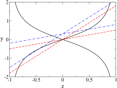
Figure 3: (Color online) Stationary solutions of the Josephson equations, represented by the intersections of the solid lines ($y=\pm\frac{z}{\sqrt{1-z^{2}}}$) with the dashed ones ($y=\Lambda z$ for $\Lambda=0.5;1.8$ - symmetric potential case) and dashed dotted line ($y=\Lambda z+\Delta$ for $\Lambda=0.5;1.8$ and $\Delta=0.3$- asymmetric potential case).

Now consider the dynamics of the $\Delta=0$ case. Constant energy contours in $z$, $\phi$ phase space followed by the system for positive $\Lambda$ are shown in Fig. 5, (A-D), one each for $\Lambda<1$, $1<\Lambda<2$ and two for $\Lambda>2$, each of which is generic. The difference between the second and third case concerns the possibility of self trapping solutions oscillating about an average $z$ such that $\phi$ covers all possible values in the third case. However, the fixed point dynamics is common to the latter three cases. Fixed points are at: (1) $z=0$, $\phi=0$; (2) $z=0$, $\phi=\pm\pi$; (3) $z=\sqrt{1-\Lambda^{-2}}$, $\phi=\pm\pi$, $\Lambda>1$. The latter pair bifurcate from the second point as we increase $\Lambda$ through $\Lambda=1$, see Fig. 3 for an illustration of how this happens.

We will now look at the stability of the three classes of fixed points. Assume perturbations such that $z\rightarrow z+\delta ze^{\lambda t}$ and $\phi\rightarrow\phi+\delta\phi e^{\lambda t}$. Simple calculations give values of $\lambda$ for the three categories:
(1) $\lambda^{2}=-(1+\Lambda)$ (phase point in the ($\phi$,$z$) plane moves on an ellipse like trajectory around ($0$,$0$))
(2) $\lambda^{2}=\Lambda-1$ (fixed point stable when $\Lambda<1$, but when $\Lambda>1$, any perturbation moves out along an arm of the separatrix emerging from ($\pm\pi$,$0$))
(3) $\lambda^{2}=1-\Lambda^{2}$ (phase point moves on an ellipse like trajectory around one of ($\pm\pi$,$\pm\sqrt{1-\Lambda^{-2}}$))
Thus, according to this criterion the first fixed point is always stable for $\Lambda>-1$. The antisymmetric solution (2) is stable for $\Lambda<1$ and unstable for $\Lambda>1$. The bifurcated pair (3) is always stable and we have a typical pitchfork bifurcation at $\Lambda=1$. These results are in full agreement with a numerical stability analysis based on the nonlinear Schrödinger equation (see Fig. 6). We might add that they contradict some statements in the literature, e.g. Dagosta and Weinstein .

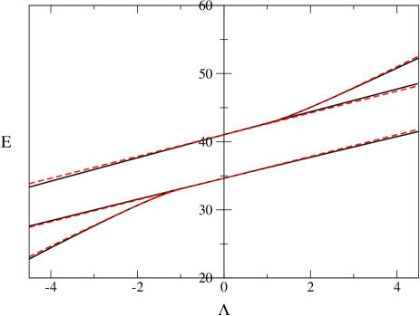
Figure 4: (Color online) Bifurcation diagram. The two sets of curves that almost coincide are obtained from the Josephson Hamiltonian (dashed lines) and the exact formulas of sections II and III (solid lines). Beyond the bifurcation point the symmetric solutions are unstable and the asymmetric ones are stable. Each point on the stable bifurcated branch corresponds to two mirror image solutions.

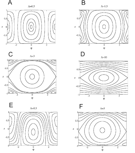
Figure 5: Phase space diagrams. The first four frames correspond to symmetric potential wells, the latter two to a deeper well on the left ($\Delta=0.3$). Note the differences in the trajectories between the cases B and E, especially in the ”waves” that cover the entire $\phi$-range. The fixed points are still present in the corners of the fourth frame (D) but do not turn up on this scale.

Figure 6: Evolution of $z(t)$ for the antisymmetric states, $\phi=\pi$: a) $\eta=-10$ , $\Lambda=-4.52$ ; b) $\eta=-1$, $\Lambda=-0.452$ ; c) $\eta=1$, $\Lambda=0.452$; d) $\eta=10$, $\Lambda=4.52$. As we see in the case of a), b) and c) the solution is stable. The periods of oscillations match the formulas derived from the values of $\lambda$ given in Section 3, $T=2\pi/|\lambda|$. In case d) the solution is unstable. The stability of the asymmetric bifurcated branch has also been confirmed.

One might wonder how the Josephson bifurcation picture ties up with the exact solutions considered earlier. Suppose we have an analytic solution given by $m_{1}$, $m_{2}$, $m_{3}$, $\mu$ and $d$. As $\phi=\pm\pi$ in our considerations, this solution clearly corresponds to one of the bifurcated fixed points in the Josephson model. How can we determine the corresponding value of $\Lambda$ so that $z$ takes the proper value? A good approximation to $z$ when $d$ is small, is (Appendix):

$$z=\frac{\left[(k_{1}^{2}-k_{3}^{2})\omega-k_{1}E(k_{1}\omega|m_{1})+k_{3}E(k_{3}\omega|m_{3})\right]}{\left[(k_{1}^{2}+k_{3}^{2})\omega-k_{1}E(k_{1}\omega|m_{1})-k_{3}E(k_{3}\omega|m_{3})\right]}$$ (33)

and $\Lambda=(1-z^{2})^{-1/2}$. The apparent independence of $d$ is deceptive, as $d$ will determine $m_{1}$ and $m_{3}$, above. In particular when $d=0$, $m_{1}=m_{3}$, $k_{1}=k_{3}$ and $z=0$ as expected. The antisymmetric solution is recovered.

When $\Lambda\neq 0$, the fixed points are still located at $\phi=0;\pm\pi$. The stationary values of $z$ are now roots of the quartic

$$\Lambda^{2}z^{4}+2\Delta\Lambda z^{3}+(\Delta^{2}+1-\Lambda^{2})z^{2}-2\Lambda\Delta z-\Delta^{2}=0$$ (34)

and are shifted down as compared to the case of $\Delta=0$. Illustrations of how phase diagrams are modified as compared to the symmetric potential case are given in Fig. 5, E and F. Now phase curves covering all possible $\phi$ values and such that $z$ changes sign are possible. As we increase $\Lambda$ from zero, a new double fixed point suddenly appears at a critical value of $\Lambda$ equal $\Lambda_{c}=(1-\Delta^{2/3})^{3/2}$, and bifurcates as we increase $\Lambda$. Thus for $\Lambda>\Lambda_{c}$ we have two new fixed points. A stability analysis yields results similar to the above, for $\Delta=0$, but values of $\lambda_{i}$ are now given in terms of roots of the quartic $z_{i}$.

VI Conclusions

In this paper we have thoroughly investigated the behavior of Bose-Einstein condensates in double square well potentials, both symmetric and asymmetric. A simple method for obtaining exact solutions for repulsive interaction was outlined (similarly as in Zin for attractive interaction). We treat the system both exactly and by a Josephson Junction model. We have checked the Josephson model results, both static and dynamic, against exact calculations. Agreement is suprisingly good. Some controversies about the stability, to be found in the literature, have been resolved.

VII Acknowledgement

The authors would like to acknowledge support from KBN Grant 2P03 B4325 (E.I.), KBN Grant 1P03B14629 (P.Z.) and the Polish Ministry of Scientific Research and Information Technology under grant PBZ-MIN-008/P03/2003 (M.T.).

Consultations with Professor George Rowlands were very helpful.

VIII Appendix

VIII.1 Symmetry preserving case (symmetric wells)

To find the $\Delta\mu$ correction we eliminate $A$ and $A_{2}$ from equations (8) and (9)

$$F=\frac{k\mbox{cn}(k\omega|m)\mbox{dn}(k\omega|m)}{\mbox{sn}(k\omega|m)}+\frac{k_{2}\mbox{dn}(k_{2}b|m_{2})}{\mbox{sn}(k_{2}b|m_{2})\mbox{cn}(k_{2}b|m_{2})}=0.$$ (35)

and calculate the perfect differential of $F(m,m_{2},\mu)$ for small $\eta$. As the first two differentials follow from Eqs. (14) $\Delta\mu$ can be so obtained. This calculation is somewhat less straightforward. It completes the calculation of $m$, $m_{2}$ and $\mu$ in the small $\eta$ limit, our starting point.

In the limit $m$ and $1-m_{2}$ tending to zero Eq. (15) is recovered from (35). The general equation for small increments of $m,m_{2}$ and $\mu$ is

$$\Delta F=\frac{\partial F}{\partial m}\Delta m+\frac{\partial F}{\partial m_{2}}\Delta m_{2}+\frac{\partial F}{\partial\mu}\Delta\mu=0$$

$$\Delta m=m,\,\,\,\,\Delta m_{2}=m_{2}-1,\,\,\,\,\Delta\mu=\mu-\mu_{0},$$ (36)

and so

$$\Delta\mu=\left(-\frac{\partial F}{\partial m}m+\frac{\partial F}{\partial m_{2}}(1-m_{2})\right)\left(\frac{\partial F}{\partial\mu}\right)^{-1},$$ (37)

where in the perturbation limit $m$ and $1-m_{2}$ are proportional to $\eta$ and are given by equation (14). We find after some calculations using known identities Abram

$$\frac{\partial F}{\partial m} = -k\left(\frac{3}{4}S+\frac{1}{4}\sin 2k\omega\right)$$

$$\frac{\partial F}{\partial m_{2}} = k_{2}\left(\frac{3}{4}L-\frac{1}{4}\sinh(2k_{2}b)\right)$$

$$\frac{\partial F}{\partial\mu} = \frac{1}{2k}S-\frac{1}{2k_{2}}L=-\frac{A^{-2}}{2\sin^{2}k\omega}$$ (38)

and

$$S = \cot(k\omega)-\frac{k\omega}{\sin^{2}(k\omega)}$$

$$L = \coth(k_{2}b)-\frac{k_{2}b}{\sinh^{2}(k_{2}b)},$$ (39)

where $k$ and $k_{2}$ are taken in the linear limit.

VIII.2 Symmetry breaking case (symmetric wells)

We obtain

$$A_{1}^{2}=\frac{2m_{1}k_{1}^{2}}{\eta},\ \ \ \ \ A_{3}^{2}=\frac{2m_{3}k_{3}^{2}}{\eta},\ \ \ \ \ \ A_{2}^{2}=\frac{2(1-m_{2})k_{2}^{2}}{\eta},$$

$$\mu=(1+m_{1})k_{1}^{2}=(1+m_{3})k_{3}^{2}=(m_{2}-2)k_{2}^{2}+V_{0}.$$ (40)

The continuity conditions at $x=\pm b$ are now generalized to:

$$g_{0} = k_{1}\sqrt{m_{1}}\,\,\mbox{sn}(k_{1}\omega|m_{1})-k_{2}\sqrt{(1-m_{2})}\,\,\mbox{sc}(k_{2}(b-d)|m_{2})=0$$ (41)

$$g_{1} = k_{3}\sqrt{m_{3}}\,\,\mbox{sn}(k_{3}\omega|m_{3})-k_{2}\sqrt{(1-m_{2})}\,\,\mbox{sc}(k_{2}(b+d)|m_{2})=0$$

$$g_{2} = k_{1}^{2}\sqrt{m_{1}}\,\,\mbox{cn}(k_{1}\omega|m_{1})\,\,\mbox{dn}(k_{1}\omega|m_{1})+k_{2}^{2}\sqrt{1-m_{2}}\,\,\mbox{dc}(k_{2}(b-d)|m_{2})\,\,\mbox{nc}(k_{2}(b-d)|m_{2})=0$$

$$g_{3} = k_{3}^{2}\sqrt{m_{3}}\,\,\mbox{cn}(k_{3}\omega|m_{3})\,\,\mbox{dn}(k_{3}\omega|m_{3})+k_{2}^{2}\sqrt{1-m_{2}}\,\,\mbox{dc}(k_{2}(b+d)|m_{2})\,\,\mbox{nc}(k_{2}(b+d)|m_{2})=0.$$

and the normalization condition is now:

$$g_{4} = {2k_{2}}\left[\mbox{sn}(k_{2}(b-d)|m_{2})\,\mbox{dc}(k_{2}(b-d)|m_{2})+\mbox{sn}(k_{2}(b+d)|m_{2})\,\mbox{dc}(k_{2}(b+d)|m_{2})\right]$$

$$-{2k_{2}}\left[E(k_{2}(b+d)|m_{2})+E(k_{2}(b-d)|m_{2})\right]$$

$$+{2k_{1}}\left[k_{1}\omega-E(k_{1}\omega|m_{1})\right]+{2k_{3}}\left[k_{3}\omega-E(k_{3}\omega|m_{3})\right]={\eta}.$$

If we can assume $k_{2}d$ much smaller than one, Eqs. (41) and (VIII.2) up to second order simplify to:

$$\chi(m_{1})-\chi(m_{3})=2D_{2}d\frac{(2-m_{2})\mbox{sc}(k_{2}b|m_{2})+2(1-m_{2})\mbox{sc}^{3}(k_{2}b|m_{2})}{m_{2}}$$ (43)

$$\chi(m_{1})+\chi(m_{3})=-\frac{2D_{2}}{k_{2}}\mbox{dc}(k_{2}b|m_{2})\mbox{nc}(k_{2}b|m_{2})$$

$$\psi(m_{1})-\psi(m_{3})=-2dk_{2}^{2}\sqrt{1-m_{2}}\mbox{dc}(k_{2}b|m_{2})\mbox{nc}(k_{2}b|m_{2})$$

$$\psi(m_{1})+\psi(m_{3})=2k_{2}\sqrt{1-m_{2}}\mbox{sc}(k_{2}b|m_{2})$$

$$\eta=\left[\phi(m_{1})+\phi(m_{3})\right]+4k_{2}\left[\mbox{sn}(k_{2}b|m_{2})\mbox{dc}(k_{2}b|m_{2})-E(k_{2}b|m_{2})\right]$$

where:

$$\chi(m) = \frac{\mu}{1+m}\sqrt{m}\,\mbox{cn}(k\omega|m)\,\mbox{dn}(k\omega|m)$$

$$\psi(m) = \sqrt{\frac{\mu}{1+m}}\sqrt{m}\,\,{\mbox{sn}(k\omega|m)}$$

$$D_{2} = \left[\frac{V_{0}-\mu}{2-m_{2}}\right]^{3/2}\sqrt{1-m_{2}}\ \ \ \ k^{2}=\frac{\mu}{1+m}\ \ \ k_{2}^{2}=\frac{V_{0}-\mu}{2-m_{2}}$$

$$\phi(m) = 2k\left[k\omega-E(k\omega|m)\right],$$

and $z=\left[\phi(m_{1})-\phi(m_{3})\right]/\left[\phi(m_{1})+\phi(m_{3})\right]$. By comparing $d$ determined by the first and third equations we can reduce the system to just four equations for four unknowns, $m_{1}$, $m_{2}$, $m_{3}$ and $\mu$.

References

- (1) K. W. Mahmud, J. N. Kutz, and W. P. Reinhardt, Phys. Rev. A 66, 063607 (2002),
- (2) P. Ziń, E. Infeld, M. Matuszewski, G. Rowlands and Marek Trippenbach, Phys. Rev. A 73, 022105 (2006).
- (3) M. Albiez, et. al, Phys. Rev. Lett. 95, 010402 (2005).
- (4) E. Sakellari, N.P. Proukakis, M. Leadbeater and C.S. Adams, New Journal of Physics 6, 42 (2004).
- (5) Elena A. Ostrovskaya, et. al, Phys. Rev. A 61, 031601(R) (2000).
- (6) S. Giovanazzi, A. Smerzi and S. Fantoni, Phys. Rev. Lett. 84, 4521 (2000).
- (7) Smerzi et al, Phys. Rev. Lett. 79, 4950 (1997).
- (8) S. Raghavan, A. Smerzi, S. Fantoni, and S. R. Shenoy, Phys. Rev. A. 59, 620 (1999).
- (9) F.S. Cataliotti, et. al, Science 293, 843 (2001).
- (10) E. B. Davies, Commun. Math. Phys. 64, 191 (1979).
- (11) J. P. G. Kevrekidis, Zhigang Chen, B. A. Malomed, D. J. Frantzeskakis and M. I. Weinstein, Physics Letters A 340, 275 (2005).
- (12) G. Ioos,D.D. Joseph, Elementary Stability and Bifurcation Theory, Springer, New York 1980.
- (13) R. D’Agosta, and C. Presilla, Phys. Rev. A 65, 043609 (2002).
- (14) M. Abramovich, I. A. Stegun, Handbook of Mathematical Functions With Formulas, Graphs and Mathematical Tables, Dover Publications, 1974.
- (15) R.K. Jackson and M.I. Weinstein, J. Stat. Phys. 116, 881 (2004).