Scattering wave function approach to multi-terminal mesoscopic system with spin-orbit coupling

Abstract

In this paper,we present a detailed formulation to solve the scattering wave function for a multi-terminal mesoscopic system with spin-orbit coupling. In addition to terminal currents, all local quantities can be calculated explicitly by taking proper ensemble average in the Landauer-Buttiker’s spirit using the scattering wave functions. Based on this formulation, we derive some rigorous results for equilibrium state. Furthermore, some new symmetry relations are found for the typical two terminal structure in which a semiconductor bar with Rashba or/and Dresselhaus SO coupling is sandwiched symmetrically between two leads. These symmetry property can provide accuracy tests for experimental measurements and numerical calculations.

I Introduction

During the past two decades, there is a fundamental progress in the understanding of transport properties in mesoscopic systemsdata . Quantum coherence in these systems plays a much more important role than in macroscopic dissipative systems. Accordingly, traditional approaches based on quasi-classical picture (e.g., Boltzmann approach) of carriers ceased to work in these systems. Fortunately, a well known new approach was built up to take into account quantum coherence adequately, i.e., Landuer-Buttiker theory(LBT)data . In this theory, a mesoscopic system under consideration is connected to electric contacts through some ideal leads and the transport properties are determined by carrier scattering probability between these leads. In practice, the central part of LBT is the quantum mechanical scattering problem for a particle incident from each lead. However, under most circumstances, only the terminal quantities are actually concerned (most real experiments probe only terminal currents instead of current density, or any other local quantities in the system). Then, all one need is the scattering matrix between the leads and the terminal conductances can be simply cast into a beautiful formula expressed by Green’s functionsdata . This formula is frequently used in literature. Up to our knowledge, no one has bothered himself previously to solve the whole scattering wave function explicitly. However, as is easy to see, the scattering wave functions are needed, if we want to calculate local properties in the Landauer-Buttiker Scenario.

Recently, there is a hot topic in the field of spintronics, called spin hall effect(SHE)Hirsch1999 ; MurakamiScience2003 ; SinovaPRL2004 . SHE refers to the phenomena that when a longitudinal electric field (or charge current) is applied in a semiconductor strip, transverse spin current and/or ensuing spin polarization near transverse boundaries can be induced. Such an effect opens a possible new way to manipulate spin degree of freedom by all-electrical means, which is a big goal to the frontier research community in semiconductor industryDassarma2004 ; semibook2002 . Some years ago, two theoretical works predicted such an effectMurakamiScience2003 ; SinovaPRL2004 as an intrinsic property of spin-orbit coupled semiconductor band structure. Since then, a lot of theoretical efforts are made to clarify some fundamental controversies in this fieldJPHu2003 ; RashbaPRB2003 ; InouePRB2004 ; MishchenkoPRL2004 ; SQShen2004 ; NikolicPRL2005 ; NikolicPRB2005 ; NikolicPRB2006 ; LShengPRL2005 ; JLi2005 ; Mlushkov05 ; HalprinPRL ; SarmaPRL ; Usaj2005 ; Sarma06 ; Ma2004 ; shijunren ; Jsinova2005 ; Zyang2005 ; YJJiang2005 . There are now also two central experimental results reporting the local measurement of opposite spin polarization near two transverse boundariesKatoScience2004 ; WunderlichPRL2005 , which have attracted many theoretical interpretations. Despite many important progresses and consensus made, there sill remain some basic difficultiesJsinova2005 .

Different theoretical approaches for spin dependent transport are employed in this field. Among them, the Landauer-Buttiker formalism is suitable to address the ballistic transport regime and has the merit of fully taking into account the phase information. This approach is in some sense mutually complementary to Boltzmann approaches based on the quasi-classical wave packet picture. Based on this approach, some important numerical results has been achieved in the topic of intrinsic SHENikolicPRL2005 ; NikolicPRB2005 ; NikolicPRB2006 ; LShengPRL2005 ; JLi2005 ; Usaj2005 ; Zyang2005 ; YJJiang2005 . However, it is worthy to point out, that most previous works based on the Landauer-Buttiker’s picture does not solve the scattering wave functions explicitlyNikolicPRL2005 ; NikolicPRB2005 ; LShengPRL2005 ; JLi2005 ; Usaj2005 . The normal green’s function formuladata compute terminal conductances but not local quantities such as spin density. On the other hand, the so called Landauer-Keldysh formalismNikolicPRL2005 ; NikolicPRB2005 ; Usaj2005 used by some authors which can compute local quantities is not manifestly single particle description and lacks intuitional simplicity. So, in order to calculate the non-equilibrium local quantities in a transparent manner, it is appealing to solve the single particle scattering wave function in the Landauer-Buttiker geometry explicitly.

In this paper, we will set up the linear equations to solve the scattering wave function in the multi-terminal Landauer geometry explicitly. With single particle wave function at hand, we can calculate any non-equilibrium local quantities(e.g.,spin density), by taking proper ensemble average in the Landuer-Buttiker spirit. Furthermore, we will derive some rigorous results in the scattering wave function description. These include: (1)deduction of the green’s function formula for terminal spin current widely used in literature, (2) rigorous proof of some important properties for equilibrium state in the Landauer’s structure, (3) revelation of some new symmetry relations in a typical two terminal structure. These symmetry property can provide accuracy tests for experimental measurements and numerical calculations.

II Description of the method to solve scattering wave function

Figure 1: schematic geometry of multi-terminal structure

We will consider a general mesoscopic structure in which a spin-orbit coupling system is attached to several ideal leads, as shown in Fig.1. The p’th lead is extending to reservoir with chemical potential $\mu_{p}$ at infinity. In a discrete representation, both the SO system and leads are modelled by a nearest neighbor tight binding(TB) Hamiltonian. We assume a tunable coupling between p’th lead and SO system by hopping interaction $t_{ps}$. The Hamiltonian for the total system reads:

$${\cal H}=H_{leads}+H_{sys}+H_{int}$$ (1)

Here, $H_{leads}=-\sum_{p}t_{p}\sum_{<p_{i},p_{j}>\sigma}(C_{p_{i}\sigma}^{{\dagger}}C_{p_{j}\sigma}+h.c.)$ is the TB Hamiltonian for the half infinite leads and $C_{p_{j}\sigma}$ denotes annihilation operator for j’th site with spin index $\sigma$ on p’th lead. $H_{int}=-\sum_{p}t_{ps}\sum_{n}(C_{p_{n}\sigma}^{{\dagger}}C_{R_{n}\sigma}+h.c.)$ describes coupling between SO system and leads, where $t_{p^{\prime}s}$ is the tunable nearest-neighbor hopping parameter between the lead $p^{\prime}$ and the SO system. ($p_{n},R_{n}$) is the nearest pair across the lead/system interface. $H_{sys}=H_{0}+H_{so}$ is the Hamiltonian for the SO coupling system in which $H_{0}=-t\sum_{<R_{i},R_{j}>\sigma}(C_{R_{i}\sigma}^{{\dagger}}C_{R_{j}\sigma}+h.c.)$ is the free band Hamiltonian,where $C_{R_{j}\sigma}$ is annihilation operator in the SO system,and $H_{so}$ denotes SO coupling term. For a typical Rashba model, we write:

$$H_{so}^{R}=-t^{R}\sum_{R_{i}}[i(\Psi_{R_{i}}^{{\dagger}}\sigma^{x}\Psi_{R_{i}+y}-\Psi_{R_{i}}^{{\dagger}}\sigma^{y}\Psi_{R_{i}+x})+h.c.]$$ (2)

Where $t^{R}$ is the Rashba coupling strength and $\Psi_{R_{i}}=(C_{R_{i},\uparrow},C_{R_{i},\downarrow})$ is the vector representation of spinor annihilation operators.

In the following, we will adopt local coordinate frame. Generally we use double coordinate index $(x_{p},y_{p}),x_{p}=1,...\infty$ and $y_{p}=1,...,N_{p}$ for sites in lead p, and $(x_{s},y_{s})$ for sites in 2DEG system.We will also use single coordinate $y$ or $y_{s}$ to represent one site on the leads or in the system when there is no risk of confusion. Furthermore, we denote $n_{py}$ as the boundary site in the system near to first row site $(x_{p}=1,y_{p})$ in lead p.

Now, suppose there is an incident wave $e^{-ik_{m}^{p}x_{p}}\chi_{m\sigma}^{p}(y_{p})$ in lead $p$ (we assume the m’th transverse mode in lead $p$ is conducting for incident energy $E$), where $k_{m}^{p}$ is the longitudinal wave vector, $\chi_{m}^{p}$ is the wave function of m’th transverse mode and $\sigma$ is the spin index of the incident carrier. Hereafter we choose z axis(normal to the 2DEG plane) as the quantization axis for spin. Generally, the wave function in lead $p^{\prime}$ can be written as:

$$\psi_{\sigma\prime}^{pm\sigma}(x_{p^{\prime}},y_{p^{\prime}})=\delta_{pp^{\prime}}\delta_{\sigma\sigma\prime}e^{-ik_{m}^{p}x_{p}}\chi_{m\sigma}^{p}(y_{p})$$

$$+\sum_{m^{\prime}\in{p^{\prime}}}\phi_{p^{\prime}m^{\prime}\sigma^{\prime}}^{pm\sigma}e^{ik_{m^{\prime}}^{p^{\prime}}x_{p^{\prime}}}\chi_{m^{\prime}\sigma^{\prime}}^{p^{\prime}}(y_{p^{\prime}})$$ (3)

where $\phi_{p^{\prime}m^{\prime}\sigma^{\prime}}^{pm\sigma}$ is the scattering amplitude from in-going mode $(m\sigma)$ in lead $p$ to out-going mode $(m^{\prime}\sigma^{\prime})$ in lead $p^{\prime}$. The longitudinal wave vectors is determined by:

$$k_{m^{\prime}}^{p^{\prime}} = \cos^{-1}(\frac{E-\varepsilon_{m^{\prime}}^{p^{\prime}}}{-2t_{p^{\prime}}}),\left|{E-\varepsilon_{m^{\prime}}^{p^{\prime}}}\right|\leq{2t_{p^{\prime}}}$$

$$k_{m^{\prime}}^{p^{\prime}} = i\cosh^{-1}(\frac{E-\varepsilon_{m^{\prime}}^{p^{\prime}}}{2t_{p^{\prime}}})+\pi,{E-\varepsilon_{m^{\prime}}^{p^{\prime}}}>{2t_{p^{\prime}}}$$

$$k_{m^{\prime}}^{p^{\prime}} = i\cosh^{-1}(\frac{E-\varepsilon_{m^{\prime}}^{p^{\prime}}}{-2t_{p^{\prime}}}),{E-\varepsilon_{m^{\prime}}^{p^{\prime}}}<{-2t_{p^{\prime}}}$$

In the Eq.(LABEL:eq:wave_vector), the first line describes real $k_{m^{\prime}}^{p^{\prime}}$ and the corresponding mode is conducting. The last two lines have imaginary $k_{m^{\prime}}^{p^{\prime}}$ value and the corresponding mode is non-conducting, or, evanescent. The evanescent mode describes local components of scattering wave function in leads which decay exponentially away from the lead/system interface. It contributes zero to terminal current. The incident energy $E$ lies out of the band continuum of such modes.

Now let’s use a column vector $\psi_{s}$ of length $2N$ ($N$ is the number of lattice sites in the SO system) to represent the wave function in the SO system $\psi_{\sigma^{\prime}}^{pm\sigma}(x_{s},y_{s})$ as a whole. Furthermore we arrange the scattering amplitudes $\phi_{p^{\prime}m^{\prime}\sigma^{\prime}}^{pm\sigma}$ into another column vector $\phi$ of length $2M$ ( $M=\sum_{p}N_{p}$ is the total number of transverse sites on all leads). Of course, these two vectors are the central quantities in our scattering problem and we want to solve them from the Schrodinger equations. As different from the continuum model, the Schrodinger equations equations has a lattice form( in real space, there is one separate equation centered on each site and spin index ) in our case and the normal boundary conditions has different appearance. Form Eq.(3) is the general linear combination of scattering eigen-states in the leads, thus for all sites on the leads except the first row sites, the Schrodinger equation is satisfied automatically. The Schrodinger equation for first row sites, however, has a different form due to its coupling with the system. On the other hand, all sites in the system has normal form of Schrodinger equation for a closed system except the boundary sites which has coupling to the first row sites in the leads. These two connecting conditions constitute the boundary condition in our problem. To be explicit,we write down Schrodinger equations centered on each site in the system and on first row of all leads separately as:

$$E\psi_{\sigma^{\prime}}^{pm\sigma}(y^{\prime}_{s}) =\sum_{y^{\prime\prime}_{s}\sigma^{\prime\prime}}H_{sys}(y^{\prime}_{s}\sigma^{\prime},y^{\prime\prime}_{s}\sigma^{\prime\prime})\psi_{\sigma^{\prime\prime}}^{pm\sigma}(y^{\prime\prime}_{s})-\sum_{p^{\prime},y}t_{p^{\prime}s}\delta_{y^{\prime}_{s},n_{p^{\prime}y}}\psi_{\sigma^{\prime}}^{pm\sigma}(1,y_{p^{\prime}})$$ (5)

$$E\psi_{\sigma^{\prime}}^{pm\sigma}(1,y^{\prime}_{p^{\prime}}) =\sum_{y^{\prime\prime}}H_{leads}(y^{\prime}_{p^{\prime}}\sigma^{\prime},y^{\prime\prime}_{p^{\prime}}\sigma^{\prime})\psi_{\sigma^{\prime}}^{pm\sigma}(y^{\prime\prime}_{p^{\prime}})-\sum_{y_{s}}t_{p^{\prime}s}\delta_{y_{s},n_{p^{\prime}y^{\prime}}}\psi_{\sigma^{\prime}}^{pm\sigma}(y_{s})$$

Note on the above equation we have used $y^{\prime}_{s},y^{\prime\prime}_{s}$ to denote a site in the system and $y^{\prime}_{p^{\prime}},y^{\prime\prime}_{p^{\prime}}$ to denote a site in lead $p^{\prime}$. However,at the same time we also used double index $(1,y^{\prime}_{p^{\prime}})$ etc. for first row sites in lead $p^{\prime}$ for clarity. $n_{p^{\prime}y^{\prime}}$ denotes the boundary site in the system near to first row site $(1,y^{\prime}_{p^{\prime}})$ of lead $p^{\prime}$. Substituting Eq.(3) into Eq.(5) and after some routine algebra, we arrive to the following matrix equations for the unknown vectors $\psi_{s}$ and $\phi$:

$$\textbf{A}\psi_{s}=\textbf{b}+\textbf{B}\phi$$ (6a)

$$\textbf{C}\phi=\textbf{d}+\textbf{D}\psi_{s}$$ (6b)

Here $\textbf{A},\textbf{B},\textbf{C},\textbf{D}$ are matrices with dimensions $2N\times 2N,2N\times 2M,2M\times 2M,2M\times 2N$ respectively. They are determined by the Hamiltonian and the geometric structure of the entire system. $\textbf{b},\textbf{d}$ are constant vectors determined by incident wave. These equations reflect the mutual influence of the leads and system through interface hopping. With some algebra, we can write down the matrix elements explicitly as following:

A $$= E-H_{sys}$$

$$\textbf{B}(n_{p^{\prime\prime}y}\sigma^{\prime\prime},p^{\prime}m^{\prime}\sigma^{\prime}) = -\delta_{p^{\prime\prime},p^{\prime}}\delta_{\sigma^{\prime\prime},\sigma^{\prime}}t_{p^{\prime}s}\chi_{m^{\prime}}^{p^{\prime}}(y_{p^{\prime\prime}})e^{ik_{m^{\prime}}^{p^{\prime}}}$$

$$\textbf{D}(p^{\prime}m^{\prime}\sigma^{\prime},n_{p^{\prime\prime}y}\sigma^{\prime\prime}) = -\delta_{p^{\prime\prime},p^{\prime}}\delta_{\sigma^{\prime\prime},\sigma^{\prime}}t_{p^{\prime}s}\chi_{m^{\prime}}^{p^{\prime}}(y_{p^{\prime\prime}})$$

$$\textbf{C}(p^{\prime}m^{\prime}\sigma^{\prime},p^{\prime\prime}m^{\prime\prime}\sigma^{\prime\prime}) = -\delta_{p^{\prime\prime},p^{\prime}}\delta_{\sigma^{\prime\prime},\sigma^{\prime}}\delta_{m^{\prime\prime}m^{\prime}}t_{p^{\prime}}$$

$$\textbf{ b}(n_{p^{\prime}y}\sigma^{\prime}) = -\delta_{pp^{\prime}}\delta_{\sigma\sigma^{\prime}}t_{ps}\chi_{m}^{p}(y_{p^{\prime}})e^{-ik_{m}^{p}}$$

$$\textbf{d}(p^{\prime}m^{\prime}\sigma^{\prime}) = \delta_{pp^{\prime}}\delta_{mm^{\prime}}\delta_{\sigma\sigma^{\prime}}t_{p}$$ (7)

The indices for lead, transverse mode, site and spin can take all possible values. All other matrix elements not included in Eq.(7) are zero. Note for some corner points in the SO system, there may be nearest neighbor points in different leads. These corner sites have multiple notation in the above scheme. However, it causes no problem because in real programming, of course, we will assign certain index to one point.

Note matrix C is diagonal and can be simply inverted. Defining matrix $\Sigma^{R}=\textbf{B}\textbf{C}^{-1}\textbf{D}$, it is easy to see that its elements are:

$$\Sigma^{R}(n_{y_{1p^{\prime}}}\sigma^{\prime},n_{y_{2p^{\prime}}}\sigma^{\prime})=-\sum\limits_{m^{\prime}}\frac{t_{p^{\prime}s}^{2}}{t_{p^{\prime}}}\chi_{m^{\prime}}^{p^{\prime}}(y_{1})\chi_{m^{\prime}}^{p^{\prime}}(y_{2})e^{ik_{m^{\prime}}^{p^{\prime}}}$$ (8)

and all other elements are zero. From Eq.(6) we have:

$$\psi_{s}=(\textbf{A}-\Sigma^{R})^{-1}(\textbf{b}+\textbf{B}\textbf{C}^{-1}\textbf{d})=G^{R}\textbf{g}$$ (9)

$G^{R}=(\textbf{A}-\Sigma^{R})^{-1}$ is, by definition,the retarded Green’s function of the system under the influence of existence of leads. In Eq.(9) we defined the effective incident wave for the boundary sites, $\textbf{g}=\textbf{b}+\textbf{B}\textbf{C}^{-1}\textbf{d}$ whose nonzero elements are:

$$\textbf{g}(n_{y_{p^{\prime}}}\sigma^{\prime})=2i\delta_{pp^{\prime}}\delta_{\sigma\sigma^{\prime}}t_{ps}\sin(k_{m}^{p})\chi_{m}^{p}(y)$$ (10)

from Eq.(6b),we have $\phi=\textbf{C}^{-1}\textbf{d}+\textbf{C}^{-1}\textbf{D}G^{R}\textbf{g}$. By expanding this expression we obtain explicitly the scattering amplitudes:

$$\phi_{p^{\prime}m^{\prime}\sigma^{\prime}}^{pm\sigma}=-\delta_{pp^{\prime}}\delta_{mm^{\prime}}\delta_{\sigma\sigma^{\prime}}+t_{p^{\prime}}^{-1}t_{p^{\prime}s}\sum_{y_{p},y_{p^{\prime}}}\chi_{m^{\prime}}^{p^{\prime}}(y_{p^{\prime}})G^{R}(n_{y_{p^{\prime}}}\sigma^{\prime},n_{y_{p}}\sigma)[2it_{ps}\sin(k_{m}^{p})\chi_{m}(y_{p})]$$ (11)

III General discussion of rigorous property

III.1 The Green’s function formula

Now let’s calculate the multi-terminal transmission probability in the Landauer-Buttiker theorydata , $T_{p^{\prime}\sigma^{\prime}}^{p\sigma}=\sum\limits_{m,m^{\prime}}\left|\phi_{p^{\prime}m^{\prime}\sigma^{\prime}}^{pm\sigma}\right|^{2}\frac{v_{p^{\prime}m^{\prime}}}{v_{pm}}$, where $v_{p^{\prime}m^{\prime}}=\frac{1}{\hbar}2t_{p^{\prime}}\sin(k_{m^{\prime}}^{p^{\prime}})$ is the velocity of mode $m^{\prime}$ in lead $p^{\prime}$. With Eq.(11), for $p\neq p^{\prime}$,we get:

$$T_{p^{\prime}\sigma^{\prime}}^{p\sigma} = \sum\limits_{m,m^{\prime}}\left|\phi_{p^{\prime}m^{\prime}\sigma^{\prime}}^{pm\sigma}\right|^{2}\frac{v_{p^{\prime}m^{\prime}}}{v_{pm}}$$ (12)

$$= Tr(\Gamma^{p}G_{\sigma\sigma^{\prime}}^{A}\Gamma^{p^{\prime}}G_{\sigma^{\prime}\sigma}^{R})$$

where

$$\Gamma^{p}(y_{p},\overline{y}_{p})=\sum\limits_{m}(\frac{t_{ps}}{t_{p}})^{2}\chi_{m}(y_{p})v_{pm}\chi_{m}(\overline{y}_{p})$$

and $G^{R}_{\sigma\sigma^{\prime}}$ and $G^{A}_{\sigma\sigma^{\prime}}$ are spin-resolved retarded and advanced Green’s functions. This is just the most frequently used Green’s function formuladata . Here we have deduced it in a rigorous manner from the scattering wave description. We point out here that self energy $\Sigma^{R}$ deduced in many text booksdata have neglected contribution from evanescent modes, while our expression in Eq.(8) with longitudinal wave vector given by Eq.(LABEL:eq:wave_vector) was rigorous.

III.2 Some rigorous property of equilibrium state

III.2.1 flowing/partial and full spectral function

Now, following Landauer’s spiritdata , we assume the reservoirs connecting the leads at infinity will feed one-way moving particles to leads according to their own chemical potential. Let’s normalize the scattering wave function $\psi^{pm\sigma}$ so that there is one particle in the incident wave, i.e., we change $e^{ik_{m}^{p}\sigma}$ to $e^{ik_{m}^{p}\sigma}/\sqrt{L}$,where $L\rightarrow\infty$ is the length of lead $p$. Meanwhile, the density of states in lead $p$ is $\frac{L}{2\pi}\frac{dk}{dE}=\frac{L}{2\pi\hbar v_{pm}}$. Now let’s we add all incident channel $(m\sigma)$ of lead $p$ with corresponding density of states(DOS). Then, we get the partial(or flowing) density of states arising from incident waves in lead $p$ as following:

$$\frac{1}{2\pi} \sum\limits_{m\sigma}\psi_{s}^{pm\sigma\ast}(y^{\prime}\sigma^{\prime})\psi_{s}^{pm\sigma}(y^{\prime}\sigma^{\prime})1/\hbar v_{pm}$$ (13)

$$=\frac{1}{2\pi} \sum\limits_{y_{1},y_{2},\sigma}G^{R}(y^{\prime}\sigma^{\prime},n_{py_{1}}\sigma)\Gamma^{p}(y_{1},y_{2})G^{A}(n_{py_{2}}\sigma,y^{\prime}\sigma^{\prime})$$

$$=\frac{1}{2\pi} A^{p}(y^{\prime}\sigma^{\prime},y^{\prime}\sigma^{\prime})$$

where we defined $A^{p}(y^{\prime}\sigma^{\prime},y^{\prime}\sigma^{\prime})$ as the partial/flowing spectral function arising from current incidence in lead $p$.

Consider the equilibrium state when all reservoirs has the same chemical potential. Then, at any energy, the carriers is incident equally from all reservoirs and we should sum up the incident lead index $p$ for scattering wave functions when calculating flowing density of states:

$$\frac{1}{2\pi} \sum\limits_{p,m\sigma}\psi_{s}^{pm\sigma\ast}(y^{\prime}\sigma^{\prime})\psi_{s}^{p,m\sigma}(y^{\prime}\sigma^{\prime})1/\hbar v_{pm}$$ (14)

$$=\frac{1}{2\pi} \sum\limits_{y_{1},y_{2}}G^{R}(y^{\prime}\sigma^{\prime},n_{y_{1}}\sigma)\Gamma(y_{1},y_{2})G^{A}(n_{y_{2}}\sigma,y^{\prime}\sigma^{\prime})$$

$n_{y_{1}},n_{y_{2}}$ refer to all boundary sites in the system which has nearest hopping term to leads, and $\Gamma=\sum\limits_{p}\Gamma^{p}$. Furthermore, we can prove an important relationdata . Since

$$\left[G^{R}\right]^{-1}-\left[G^{A}\right]^{-1}=\Sigma^{A}-\Sigma^{R}=i\sum\limits_{p}\Gamma^{p}=i\Gamma$$

then,

$$G^{A}-G^{R}=iG^{R}\Gamma G^{A}\equiv iA$$

where $A=i(G^{R}-G^{A})$ is the full spectral function which plays a role of a generalized density of states inside the SO system taking the presence of all leads into account. In an open system, it’s not absolute clear how to define state and density of states. Here through our deduction we have made explicit the physical meaning of $A$ from the wave function description. We emphasize the particular boundary condition used in the leads, i.e., there is a thermal reservoir with the same chemical potential $\mu$, in the far end for every lead, in the Landauer-Buttiker sense. For non-equilibrium state, i.e., not all of the leads have same chemical potential and there will be net current in the leads and system. At that time,we are interested in flowing density $A^{p}$ rather than total density $A$.

On the above we used only the diagonal elements of $A^{p}$ and $A$. It is convenient to define the non-diagonal elements as flowing spin density density matrix:

$$A^{p}(y^{\prime}\alpha, y^{\prime\prime}\beta)=\sum\limits_{m\sigma}\psi_{s}^{\ast}(y^{\prime\prime}\beta)\psi_{s}(y^{\prime}\alpha)1/\hbar v_{pm}$$ (15)

$$= \sum\limits_{y_{1},y_{2},\sigma}G^{R}(y^{\prime}\alpha,n_{y_{1p}}\sigma)\Gamma^{p}(y_{1},y_{2})G^{A}(n_{y_{2p}}\sigma,y^{\prime\prime}\beta)$$

$$A(y^{\prime}\alpha, y^{\prime\prime}\beta)=\sum\limits_{p,m\sigma}\psi_{s}^{\ast}(y^{\prime\prime}\beta)\psi_{s}(y^{\prime}\alpha)1/\hbar v_{pm}$$

$$= \sum\limits_{p,y_{1},y_{2},\sigma}G^{R}(y^{\prime}\alpha,n_{y_{1p}}\sigma)\Gamma(y_{1},y_{2})G^{A}(n_{y_{2p}}\sigma,y^{\prime\prime}\beta)$$

$$= i(G^{R}(y^{\prime}\alpha,y^{\prime\prime}\beta)-G^{A}(y^{\prime}\alpha,y^{\prime\prime}\beta))$$

III.2.2 All $T$ odd quantities vanishes in time reversal symmetric system

Now let’s prove that in the Landauer-Buttiker description, for a time-reversal symmetric Hamiltonian, all $T$-odd quantities in equilibrium are zero:

Consider a local quantity:

$$\hat{O}^{ij}=\sum_{\alpha\beta}(C_{i\alpha}^{\dagger}O_{\alpha\beta}^{ij}C_{j\beta}+C_{j\alpha}^{\dagger}O_{\alpha\beta}^{ji}C_{i\beta})$$ (16)

Typical examples: (1)for spin density on site i, we choose $O^{ij}=\frac{\hbar}{4}\delta_{ij}\vec{\sigma}$. (2)for normally defined charge current on link $(i,j)$, we set $O^{ij}=-O^{ji}=ieI_{2\times 2}$ where $I_{2\times 2}$ is the 2d unit matrix, (3)for normally defined spin current on link $(i,j)$, we have $O^{ij}=-O^{ji}=\frac{\hbar}{2}i\vec{\sigma}$. In general we require $O^{ij}=O^{ji\dagger}$ for physical quantity.

Under time reversal manipulation, $\emph{T}=i\sigma_{y}K$, where $K$ is the conjugate operator, $\hat{O}^{ij}$ will transform as $O^{ij}_{\alpha\beta}\rightarrow(-1)^{\alpha+\beta}O_{\bar{\alpha}\bar{\beta}}^{ij*}$. There are two classes of physical quantities, depending on their symmetry under time reversal operation, i.e., either $T$-even or $T$-odd quantities. Spin density and normally defined link currents are $T$-odd quantities. In contrast, the normally defined spin currents are $T$-even quantity.

Now, let’s calculate the expectation value of $\hat{O}^{ij}$ in mesoscopic equilibrium state. By definition, this expectation value per energy interval is:

$$\langle\hat{O}^{ij}\rangle = \frac{1}{2\pi}\sum\limits_{pm\sigma}\psi_{s}^{pm\sigma\ast}(i\alpha)O_{\alpha\beta}^{ij}\psi_{s}^{pm\sigma}(j\beta)1/\hbar v_{pm}+h.c.$$

$$= \frac{1}{2\pi}\sum_{\alpha\beta}[A(j\beta,i\alpha)O_{\alpha\beta}^{ij}+h.c.]$$

$$= \frac{1}{2\pi}i\sum_{\alpha\beta}[(G^{R}-G^{A})_{j\beta,i\alpha}O_{\alpha\beta}^{ij}+(G^{R}-G^{A})_{i\alpha,j\beta}O_{\beta\alpha}^{ji}]$$

where we have used the relation $(G^{R}){\dagger}=G^{A}$. Moreover,the matrices $(G^{R})$ and $G^{A}$ are related by time reversal operation. Generally, by definition, we have:

$$(TG^{R}_{B}T^{-1})_{i\alpha,j\beta}=(-1)^{\alpha+\beta}G_{i\bar{\alpha},j\bar{\beta}}^{R*}(B)=G_{j\beta,i\alpha}^{A}(-B)$$

Here, for generality of discussion, we have used magnetic field B to break $T$ symmetry explicitly. Furthermore, let’s suppose that the Hamiltonian is $T$ invariant, then

$$(TG^{R}T^{-1})_{i\alpha,j\beta}=(-1)^{\alpha+\beta}G_{i\bar{\alpha},j\bar{\beta}}^{R*}=G_{j\beta,i\alpha}^{A}$$ (18)

The four terms in Eq.(LABEL:eq:21) can be grouped into two pairs,

$$\sum_{\alpha\beta}[G^{R}_{j\beta,i\alpha}O_{\alpha\beta}^{ij}-G^{A}_{i\alpha,j\beta}O_{\beta\alpha}^{ji}]+\sum_{\alpha\beta}[-G^{A}_{j\beta,i\alpha}O_{\alpha\beta}^{ij}+G^{R}_{i\alpha,j\beta}O_{\beta\alpha}^{ji}]$$

$$=\sum_{\alpha\beta}[G^{R}_{j\beta,i\alpha}O_{\alpha\beta}^{ij}-(-1)^{\alpha+\beta}G^{R*}_{j\bar{\beta},i\bar{\alpha}}O_{\alpha\beta}^{ij*}]+\sum_{\alpha\beta}[-(-1)^{\alpha+\beta}G^{R*}_{i\bar{\alpha},j\bar{\beta}}O_{\beta\alpha}^{ji*}+G^{R}_{i\alpha,j\beta}O_{\beta\alpha}^{ji}]$$

Now, suppose $\hat{O}$ is $T$ odd, then, $(-1)^{\alpha+\beta}O_{\alpha\beta}^{ij*}=-O_{\bar{\alpha}\bar{\beta}}^{ij}$ . Thus we have

$$\sum_{\alpha\beta}[G^{R}_{j\beta,i\alpha}O_{\alpha\beta}^{ij}-G^{A}_{i\alpha,j\beta}O_{\beta\alpha}^{ji}]+\sum_{\alpha\beta}[-G^{A}_{j\beta,i\alpha}O_{\alpha\beta}^{ij}+G^{R}_{i\alpha,j\beta}O_{\beta\alpha}^{ji}]$$

$$=\sum_{\alpha\beta}[G^{R}_{j\beta,i\alpha}O_{\alpha\beta}^{ij}+G^{R*}_{j\bar{\beta},i\bar{\alpha}}O_{\bar{\alpha}\bar{\beta}}^{ij*}]+\sum_{\alpha\beta}[G^{R*}_{i\bar{\alpha},j\bar{\beta}}O_{\bar{\beta}\bar{\alpha}}^{ji*}+G^{R}_{i\alpha,j\beta}O_{\beta\alpha}^{ji}]$$ (19)

evidently, each summation on the right hand side of Eq.(19) is real. So, the average value for physical quantity in Eq.(LABEL:eq:21) should be zero.

On the above we have proved that for any time reversal symmetric system, all $T$-odd quantities, such as spin density and local charge current, vanish in equilibrium state. This result seems to be a transparent truth. However, up to our knowledge, though many people accept it to be true, no one has proved it rigorously in Landauer’s mesoscopic structure. The corresponding fact for a closed system in equilibrium is trivial, because in closed system, each quantum state has its $T$ partner state(except the $T$ invariant states for which the average of $T$-odd operator should be zero), thus for a $T$-odd operator, the sum of average is zero. However, in our open system case, for equilibrium state, we have an ensemble of scattering wave functions incident from all leads at fermi energy while all the states are not manifestly $T$ paired.

Under finite terminal bias, the system is driven into non-equilibrium state. Due to above property, the value of $T$-odd quantity is determined by fermi surface property for small bias. This is in accordance with fermi liquid theory. But for $T$-even quantities, e.g., spin current, we cannot reach to such a conclusion. In fact, we need other symmetry considerations to interpret some $T$-even quantities to be fermi surface propertyNikolicPRB2006 .

For later use, let’s consider a geometrically symmetric system with double terminals, as shown in Fig.2. Since the spin density vanishes in equilibrium state, according to Eq.(LABEL:eq:21)we have:

$$<S_{\alpha}(x,y)>_{eq}=<S_{\alpha}(x,y)>_{I}+<S_{\alpha}(x,y)>_{-I}=0$$ (20)

where $<S_{\alpha}(x,y)>_{I}$ means partial/flowing average of spin density due to scattering states incident from lead 1, and $<S_{\alpha}(x,y)>_{-I}$ means flowing spin density due to scattering waves incident from lead 2. This relationship will be employed to derive an important symmetry properties in next section.

Figure 2: schematic geometry of two-terminal structure

III.2.3 equilibrium terminal spin current is always zero

Next, for ease of reference, we will give a explicit proof that terminal spin current also vanishes in equilibrium state(which is known by othersthank ), irrespective of the $T$ symmetry of the Hamiltonian. In linear transport regime, we neglect the energy dependence of scattering matrices, then the terminal spin current polarized in $\sigma$ direction in $p$’th lead can be calculated as,

$$I_{p}^{\sigma}=-\frac{e}{4\pi}\{\sum_{q\sigma^{\prime}}^{\prime}[(T_{p\sigma}^{q\sigma^{\prime}}-T_{p\overline{\sigma}}^{q\sigma^{\prime}})V_{q}-(T_{q\sigma^{\prime}}^{p\sigma}-T_{q\sigma^{\prime}}^{p\overline{\sigma}})V_{p}]$$

$$+2(R_{p\sigma}^{p\overline{\sigma}}-R_{p\overline{\sigma}}^{p\sigma})V_{p}\}$$ (21)

Where we used symbol $R$ to represent reflection probability in lead $p$, i.e., we define $R_{p\sigma}^{p\overline{\sigma}}=T_{p\sigma}^{p\overline{\sigma}}$ etc for clarity. On the above equation, the summation is taken over all terminals except $p$. The second term in {$\cdots$} describes contribution to spin current due to injection and reflection wave in $p$’th lead. This term is zero for normal current, where summation of all spin indices is performed.

For equilibrium state, we have $V_{q}=$constant for all $q$. Let’s firstly write down the following identities:

$$-\sum\limits_{q\sigma^{\prime}}^{\prime}T_{q\sigma^{\prime}}^{p\sigma}-R_{p\overline{\sigma}}^{p\sigma}-R_{p\sigma}^{p\sigma}=-M_{p}$$

$$\sum\limits_{q\sigma^{\prime}}^{\prime}T_{q\sigma^{\prime}}^{p\overline{\sigma}}+R_{p\sigma}^{p\overline{\sigma}}+R_{p\overline{\sigma}}^{p\overline{\sigma}}=M_{p}$$

$$\sum\limits_{q\sigma^{\prime}}^{\prime}T_{p\sigma}^{q\sigma^{\prime}}+R_{p\sigma}^{p\overline{\sigma}}+R_{p\sigma}^{p\sigma}=M_{p}$$

$$-\sum\limits_{q\sigma^{\prime}}^{\prime}T_{p\overline{\sigma}}^{q\sigma^{\prime}}-R_{p\overline{\sigma}}^{p\overline{\sigma}}-R_{p\overline{\sigma}}^{p\sigma}=-M_{p}$$

Here $M_{p}$ denotes the number of conducting mode in lead $p$. The first two equations are simple sum rules. They describe current conservation: one incident electron in lead $p$ must go somewhere. The last two equations follows from the unitarity of scattering matrix. Or,we can deduce them from the first two since $T_{p\sigma}^{q\sigma^{\prime}}(B)=T_{q\overline{\sigma}^{\prime}}^{p\overline{\sigma}}(-B)$,$R_{p\sigma}^{p\sigma^{\prime}}(B)=R_{p\sigma^{\prime}}^{p\sigma}(-B)$ due to $T$ transformation property of scattering amplitudes. Adding up all the above equations we get $I_{p(eq)}^{\sigma}=0$.

Thus, we have showed explicitly that terminal equilibrium spin currents are identically zero, irrespective of details of Hamiltonian of the system(even in the presence of magnetic field) and geometry structure. This result is parallel to the fact that terminal equilibrium charge current always vanish, while current density may be nonzero inside system when the system is placed under magnetic field.

E.I.Rashba pointed outRashbaPRB2003 that in a bulk 2DEG system with pure Rashba type of SO coupling, in-plane polarized spin current may have non-zero value in equilibrium. This simple result raised the problem of how to define spin current properly in SO systems. A much concerned problem is that whether such background spin current useful? From the practical point of view, the useful quantity is terminal spin currentpareek . In a conceived all-electric devise, we should add nonmagnetic contact to induct spin current out of SO system. However, according to the above rigorous result, the resulting equilibrium spin current in added terminals around the SO system should always vanish and we cannot simply make use of it. How does spin current decay abruptly at the boundary between lead and bulk system is an interesting problem to be clarified. Such an understanding may help to bridge the apparent gap between mesoscopic approaches and macroscopic approachesJsinova2005 (say, linear response approach).

When there is current flowing through the SO system, there will be induced spin current on attached leads. In the following we will discuss some symmetry property of such spin currents in a two terminal structure. We will reveal an emergent continuity property of spin currents due to symmetry of geometry and SO Hamiltonian.

For later use, here we write down the following equation for a two terminal system:

$$I_{2(eq)}^{\sigma}=I_{2(I)}^{\sigma}+I_{2(-I)}^{\sigma}=0$$ (23)

where $I_{2(eq)}^{\sigma}$ is the equilibrium spin current in lead 2, and $I_{2(I)}^{\sigma}$ and $I_{2(-I)}^{\sigma}$ denote spin current in lead 2 under the condition of fixed charge current I (flowing from lead $1\rightarrow 2$) and -I (flowing from lead $2\rightarrow 1$) respectively.

IV Some symmetry property of typical Spin-orbit coupling systems

Now let’s discuss the symmetry of typical Spin-orbit coupling system in which a SO bar is symmetrically attached by two ideal leads. Let’s model the SO bar by a Rashba Hamiltonian, $H_{so}=\alpha(\hat{\sigma}\times\vec{k})\cdot\vec{z}$, whose discrete version is just Eq.(2). We assume a rectangular geometry as shown in Fig 2. Firstly, let’s analyze symmetry properties of the model Hamiltonian. For pure system, it’s easy to see from Fig.2 and Eq.(1), Eq.(2), that the Hamiltonian has combined symmetry of real space reflection and spin space rotation: $\sigma_{y}P_{x}$ and $\sigma_{x}P_{y}$, where $P_{x}$ and $P_{y}$ denotes real space reflection $y\Rightarrow-y$ and $x\Rightarrow-x$, respectively, $\sigma_{x}$ and $\sigma_{y}$ acting on spinor wave function on every site are spin rotational manipulation around $x$ axis and $y$ axis, respectively. Moreover, when there is no external magnetic field, the Hamiltonian for the entire system is $T$ symmetric. From these symmetries, we can obtain the following symmetry relations:

$$<S_{x,z}(x,y)>_{I} = -<S_{x,z}(x,-y)>_{I}$$

$$<S_{y}(x,y)>_{I} = <S_{y}(x,-y)>_{I}$$

$$<S_{x}(x,y)>_{I} = -<S_{x}(-x,y)>_{I}$$

$$<S_{y,z}(x,y)>_{I} = <S_{y,z}(-x,y)>_{I}$$ (24)

$<\cdots>_{I}$ means taking ensemble average for given longitudinal current $I$ incident from lead 1. The first two lines are results of symmetry $\sigma_{y}P_{x}$ which has been known widely beforeseeSQShen2004 . The second two, however, are results from $\sigma_{x}P_{y}$ and $T$ symmetry together. From $\sigma_{x}P_{y}$, we get:$<S_{y,z}(x,y)>_{I}=-<S_{y,z}(-x,y)>_{-I},<S_{x}(x,y)>_{I}=<S_{x}(-x,y)>_{-I}$. From time reversal symmetry,we have Eq.(20). Combining these two, we obtain the last two lines in Eq.(24).

Similar symmetry relations can be easily obtained for Dresselhaus SO coupling modelSQShen2004 for which the discrete Hamiltonian reads:

$$H_{so}^{D}=t^{D}\sum_{R_{i}}[i(\Psi_{R_{i}}^{{\dagger}}\sigma^{y}\Psi_{R_{i}+y}-\Psi_{R_{i}}^{{\dagger}}\sigma^{x}\Psi_{R_{i}+x})+h.c.]$$ (25)

As can be easily seen, we have symmetry $\sigma_{x}P_{x}$, $\sigma_{y}P_{y}$ and $T$ in this Dresselhaus model. In this case, we get the following symmetry relations:

$$<S_{y,z}(x,y)>_{I} = -<S_{y,z}(x,-y)>_{I}$$

$$<S_{x}(x,y)>_{I} = <S_{x}(x,-y)>_{I}$$

$$<S_{y}(x,y)>_{I} = -<S_{y}(-x,y)>_{I}$$

$$<S_{x,z}(x,y)>_{I} = <S_{x,z}(-x,y)>_{I}$$ (26)

In the presence of both $H_{so}^{R}$ and $H_{so}^{D}$ with geometry shown in Fig.2, it can be checked easily that the total Hamiltonian is invariant under $\sigma_{z}P_{x}P_{y}$. Thus we have symmetry relations:

$$<S_{z}(x,y)>_{I} = -<S_{z}(-x,-y)>_{I}$$

$$<S_{x,y}(x,y)>_{I} = <S_{x,y}(-x,-y)>_{I}$$

Up to our knowledge, not all of the symmetry relations Eq.(24), Eq.(26) and Eq.(LABEL:eq:symmetryRD) have been reported previously. In particular, Eq.(LABEL:eq:symmetryRD) and the last two lines in Eq.(24) as well as in Eq.(26) follow from $T$ symmetry together with geometric symmetry( spacial reflection combining a spin rotation manipulation) are firstly found in this paper. These relations provide important accuracy test for experimental measurements and numerical calculations. For example, for a two-terminal structure with Rashba coupling in the middle SO bar, the theoretical assertion made in NikolicPRL2005 that longitudinal spin component is insensitive to the reversal of the bias voltage is contrary to our Eq.(20), the numerical resultNikolicPRL2005 that spin density $<S_{z}(x,y)>_{V}$ is not symmetric with $x\rightarrow{-x}$ is contrary to the last line of Eq.(24).

The issue of spin current has triggered hot discussion recently. The central problem lies in that spin is non-conservative in spin-orbit coupling system. In bulk systems, proper definition and physical consequence of spin current are currently under debate. However, in a multi-terminal structure, spin current on the leads can be defined unambiguously. In the following let’s analyze the symmetry of spin current in two terminal structure with geometric symmetry( spacial reflection combining a spin rotation manipulation). The terminal spin current on a particular lead was a summation of link spin current(see discussion below Eq.(16)) in transverse direction. Then, for a system with both $H_{so}^{R}$ and $H_{so}^{D}$ present, by taking into account Eq.(23) together with geometry symmetry and following similar argument in the derivation of symmetry relations for spin density, we get a symmetry relation similar to Eq.(LABEL:eq:symmetryRD):

$$I_{2(I)}^{z} =-I_{1(I)}^{z}$$ (28)

$$I_{2(I)}^{x,y} =I_{1(I)}^{x,y}$$

Such symmetry of terminal spin current is directly related to symmetry of spin polarization Eq.(LABEL:eq:symmetryRD) since the terminal spin current can be imagined to be injected from boundary spin density. The symmetry connection between these two quantities is clearly depicted in Fig.(3).

Figure 3: schematic picture of symmetric relation between boundary spin density and terminal spin current in a two-terminal structure

Interestingly, $I_{2(I)}^{z}$ can be interpreted as conserved current because the quantity of it injecting into and leaving out of the SO region is identical. This emergent continuity property, however, is the result of geometric symmetry. In contrast to a recently proposed spin current definitionshijunren in bulk system, for which a coarse graining process(though physically beautiful, such process is hard to done rigorously) is necessary, the continuity of spin current in our case is due to dynamical and geometric symmetry. This interpretation has at least the advantage of physical transparency. The different property of terminal spin current polarized normal and parallel to the 2DEG plane is an interesting topic to discuss. As mentioned on the above, the equilibrium in-plane spin current is not useable in an all-electric device. Under the condition of flowing current in an ideal system, terminal in-plane spin current lacks a simple physical interpretation as a current while the out-of-plane spin current does. From these simple symmetry relations, we believe these components may play very different role in spin transportation in real systems. It is interesting to consider more geometries to further expose such symmetry differences and study the different role of in-plane and out-of-plane spin current to spin transportation in real dissipative systems.

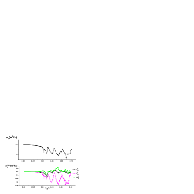
Figure 4: The charge and spin conductances as a function of Rashba coupling constant $t_{R}$. The system is taken to be $100\times 40$ sized and Dresselhaus coupling constant is fixed to be 0.02t

To have a quantitative impression on spin current, we performed some numerical calculation. Let’s consider a two-terminal system with both Rashba and Dresselhaus coupling. We adopt a discrete representation and fix $t^{D}/t=0.02$. The current is assumed to flow from lead 1 to lead 2 for a system with $100\times 40$ lattice sites and both leads are of the same width as system, the charge conductance $\sigma_{c}$ and spin conductances $\sigma_{s}^{x,y,z}$ are shown in Fig.(4). The spin conductances are much smaller compared to charge conductances and both of them oscillate rapidly in large $t_{R}/t_{D}$ regime. For $t_{R}/t_{D}<2$, $\sigma_{c}$ decreases smoothly and $\sigma_{s}^{x,y,z}$ are very small. When $t_{R}/t_{D}>2$, both $\sigma_{c}$ and $\sigma_{s}^{x,y,z}$ lines will show series of peak structures. The line-shape of $\sigma_{s}^{y}$ will follow closely to that of $\sigma_{c}$. On the other hand, the $\sigma_{s}^{x,z}$ values will decrease in the large $t_{R}$ regime due to symmetry property stated below. Once spin current become experimentally detectable, the peaks structures in the Fig.(4) are on the first place to be verified.

For pure Rashba system, due to $y\rightarrow-y$ symmetry(combining spin rotation) we have:

$$I_{2(I)}^{x,z} =I_{1(I)}^{x,z}=0$$ (29)

$$I_{2(I)}^{y} =I_{1(I)}^{y}$$

similarly, for pure Dresselhaus system, we have:

$$I_{2(I)}^{y,z} =I_{1(I)}^{y,z}=0$$ (30)

$$I_{2(I)}^{x} =I_{1(I)}^{x}$$

The symmetry relations Eq.(28),(29),(30) can hold even in the presence of magnetic field(which keep geometry symmetry), since Eq.(23) is independent of $T$ symmetry.

On the above we have obtained some new symmetry relations relating to spin polarization as well as terminal spin currents for a two-terminal structure. Some other symmetries for a two-terminal waveguide in the presence of magnetic field modulations is obtained in Ref.zhaifeng . All these symmetry relations may find application in the study of spin transport theory.

V conclusion

To sum up, we have set up a detailed formulation to solve explicitly the scattering wave functions in a multi-terminal spin-orbit coupled system. We deduced some analytical properties in the scattering wave function description of mesoscopic physics following Landauer’s spirit. In particular, we have (1) deduced rigorously the much used Green’s function formula. (2) proved rigorously that all equilibrium value of $T$-odd quantities vanish in the open multi-terminal structure. (3) reveal some new symmetry relations for two-terminal structure when the system has a Rashba or/and Dresselhaus form of SO coupling. These symmetry relations may provide accuracy test to experimental measurements and symmetry restriction to numerical calculations.