Excitonic gap, phase transition, and quantum Hall effect in graphene

Abstract

We suggest that physics underlying the recently observed removal of sublattice and spin degeneracies in graphene in a strong magnetic field describes a phase transition connected with the generation of an excitonic gap. The experimental form of the Hall conductivity is reproduced and the main characteristics of the dynamics are described. Predictions of the behavior of the gap as a function of temperature and a gate voltage are made.

I Introduction

The properties of graphene, a single atomic layer of graphite Geim2004Science , have recently attracted a lot of attention, especially after the experimental discovery Geim2005Nature ; Kim2005Nature and (independently of that) theoretical prediction Gusynin2005PRL ; Peres2005 of an anomalous quantization in the quantum Hall (QH) effect (for earlier considerations of the QH effect in graphene, see Ref. Haldane1988PRL ). The graphene material is unique because of its band structure with two inequivalent Dirac points at the corners of the Brillouin zone. As a result, its low-energy excitations are described by effective “relativistic-like” Dirac equation where the speed of light is replaced by the Fermi velocity $v_{F}$ Semenoff1984PRL .

These relativistic-like features of graphene are at the heart of the anomalous integer QH effect. In this case, the filling factors are $\nu=\pm 4(|n|+1/2)$, where $n$ is the Landau level index. For each QH state, a four-fold degeneracy takes place: it is the sublattice and spin degeneracy for the lowest Landau level (LLL) with $n=0$ and the valley and spin degeneracy for higher Landau levels (LLs) with $|n|>0$. In the very recent experiments Zhang2006 , it has been observed that in a strong enough magnetic field the new QH plateaus, $\nu=0,\pm 1$ and $\pm 4$, occur, that was attributed to the magnetic field induced splitting of the LLL and the $n=\pm 1$ LLs. It is noticeable that while the degeneracy of the lowest LLL is completely lifted, only the spin degeneracy of the $n=\pm 1$ LLs is removed.

In this paper, we suggest that the origin of the plateaus $\nu=0$ and, especially, $\nu=\pm 1$ is deeply connected with a phase transition with respect to the chemical potential $\mu$ related to the charge density of carriers (in the experiments Geim2004Science ; Geim2005Nature ; Kim2005Nature ; Zhang2006 , the chemical potential is tunable by a gate bias voltage $V_{g}$). This phase transition is provided by dynamics responsible for creating an excitonic gap $\Delta$ in a strong magnetic field: While at small $|\mu|$ the excitonic gap is generated, there is no gap as $|\mu|$ becomes larger than a critical value $|\mu_{c}|$ determined below. In fact, if this scenario is correct, the phenomenon discovered in Zhang2006 can be interpreted as the observation of two different phases in graphene.

As will be shown below, one of the predictions of this scenario is that the only plateaus in the Hall conductivity $\sigma_{xy}$ are those with $\nu=0,\pm 1$ and $\nu=\pm 2k$, $k=1,2,$…, i.e., the plateaus observed in Ref. Zhang2006 . The plateau $\nu=\pm 1$ appears only if both the spin splitting is included and the gap $\Delta$ is nonvanishing. Another prediction is that the excitonic gap $\Delta$ is much smaller than the gap $\sqrt{2\hbar v_{F}^{2}|eB|/c}$ between the LLL and the $n=\pm 1$ LLs. In other words, the excitonic gap is produced by weak coupling dynamics footnote1 . This prediction can be checked by measuring the critical temperature at which the $\nu=0$ and $\nu=\pm 1$ plateaus disappear. We also succeeded in reproducing the experimental form of $\sigma_{xy}$ obtained in Zhang2006 .

The fact that a magnetic field is a strong catalyst of electron-hole (fermion-antifermion in field theory) pairing was established long ago Gusynin1995PRD (the phenomenon was called the magnetic catalysis). The essence of this effect is the dimensional reduction $D\to D-2$ in the dynamics of electron-hole pairing: In a strong magnetic field, this pairing is mostly provided by the LLL whose dynamics is essentially $(D-2)$-dimensional. The dimensional reduction leads to a strong enhancement of the density of states. As a result, for $D=2$, as in graphene, the pairing dynamics in infrared becomes very strong and, for zero temperature and zero chemical potential, an excitonic gap is generated even at the weakest attractive interaction between electrons and holes footnote2 . Because of this feature, the phenomenon is robust. It was also shown in Ref. Gusynin1995PRD , that at large temperature or/and charge density (chemical potential), the excitonic gap disappears. As will be discussed below, it also disappears for a large impurity scattering rate.

In graphene, the phenomenon of the magnetic catalysis was considered in Refs. Khveshchenko2001PRL ; Gorbar2002PRB in connection with an interpretation of experiments in highly oriented pyrolytic graphite kopel1 . In particular, in Ref. Gorbar2002PRB , the role of temperature and chemical potential in this dynamics was clarified in detail. Also in that paper, expressions both for the diagonal conductivity $\sigma_{xx}$ and the Hall conductivity $\sigma_{xy}$ at nonzero gap $\Delta$ were derived and investigated. For further studies of this phenomenon in graphene, see Refs. Gorbar2003PLA ; Khveshchenko2004nb .

Fig. 1 illustrates the main results of our analysis. It shows the spectrum and the Hall conductivity $\sigma_{xy}$ in the $n=0$ and $n=1$ LLs for four different cases corresponding to zero (nonzero) gap $\Delta$ and spin splitting. As one can see in Fig. 1d, when both $\Delta$ and spin splitting being nonzero, the plateaus in $\sigma_{xy}$ observed in Ref. Zhang2006 are reproduced. Note that the degeneracies of the LLL and higher LLs shown in Fig. 1d are different. The physics underlying Fig. 1 will be discussed in detail in Secs. II and III below.

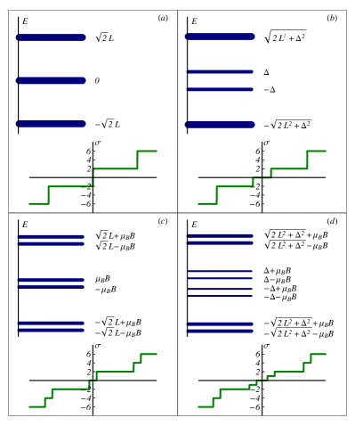
Figure 1: Schematic illustration of the spectrum and the Hall conductivity in the $n=0$ and $n=1$ Landau levels for four different cases. (a) $\Delta=0$ and no Zeeman term. (b) Nonzero $\Delta$ and no Zeeman term. (c) $\Delta=0$ and the Zeeman term is taken into account. (d) Both $\Delta$ and the Zeeman term are nonzero. Thickness of the lines represents the degeneracy $\times 4,\times 2$, and $\times 1$ of the energy states; $L=\sqrt{\hbar v_{F}^{2}|eB|/c}$.

The paper is organized as follows. In Sec. II, we consider the dynamics of the Hall conductivity in graphene when the Zeeman term is ignored (no spin splitting). In Sec. III, the realistic case, with the spin splitting taken into account, is considered. In Sec. IV, the main results of the paper are summarized. In Appendices A, B, and C, some useful formulas and relations are derived.

II Dynamics with no spin splitting

For the description of the dynamics in graphene, we will use the same model as in Refs. Khveshchenko2001PRL ; Gorbar2002PRB , the so called reduced QED. In such a model, while quasiparticles are confined to a 2-dimensional plane, the electromagnetic (Coulomb) interaction between them is three-dimensional in nature. The low-energy quasiparticles excitations in graphene are conveniently described in terms of a four-component Dirac spinor $\Psi_{\sigma}^{T}=\left(\psi_{KA\sigma},\psi_{KB\sigma},\psi_{K^{\prime}B\sigma},\psi_{K^{\prime}A\sigma}\right)$ which combines the Bloch states with spin $\sigma=\pm 1$ on the two different sublattices ($A,B$) of the hexagonal graphene lattice and with momenta near the two inequivalent points ($K,K^{\prime}$) at the opposite corners of the two-dimensional Brillouin zone. The free quasiparticle Hamiltonian can be recast in the ”relativistic” - like form with the Fermi velocity $v_{F}\approx 10^{6}\mbox{m/s}$ playing the role of the speed of light:

$$H_{0}=-iv_{F}\int d^{2}{\bf r}\,\overline{\Psi}_{\sigma}\left(\gamma^{1}\hbar\nabla_{x}+\gamma^{2}\hbar\nabla_{y}\right)\Psi_{\sigma},$$ (1)

where $\overline{\Psi}_{\sigma}=\Psi^{\dagger}_{\sigma}\gamma^{0}$ is the Dirac conjugated spinor and summation over spin $\sigma$ is understood. In Eq.(1) $\gamma^{\nu}$ with $\nu=0,1,2$ are $4\times 4$ gamma matrices belonging to a reducible representation $\gamma^{\nu}=\tilde{\tau}_{3}\otimes(\tau_{3},i\tau_{2},-i\tau_{1})$ where the Pauli matrices $\tilde{\tau},\tau$ act in the subspaces of the valley ($K,K^{\prime}$) and sublattices ($A,B$) indices, respectively. The matrices satisfy the usual anticommutation relations $\left\{\gamma^{\mu},\gamma^{\nu}\right\}=2g^{\mu\nu}$, $g^{\mu\nu}=(1,-1,-1),\mu,\nu=0,1,2$. The covariant derivative ${\boldsymbol{\nabla}}={\boldsymbol{\partial}}+(ie/\hbar c){\bf A}$ includes the vector potential in the symmetric gauge ${\bf A}^{ext}=\left(-By/2,Bx/2\right)$ corresponding to the external magnetic field applied perpendicular to the plane along the positive $z$ axis. In the four-component spinor representation, the Coulomb interaction has the form

$$H_{int}= \frac{\hbar v_{F}}{2} \int d^{2}{\bf r}d^{2}{\bf r}^{\prime}\overline{\Psi}_{\sigma}({\bf r})\gamma^{0}\Psi_{\sigma}({\bf r})\frac{g}{|{\bf r}-{\bf r}^{\prime}|}$$ (2)

$$\times \overline{\Psi}_{\sigma\prime}({\bf r})\gamma^{0}\Psi_{\sigma^{\prime}}({\bf r}),$$

where the coupling $g={e^{2}}/{\epsilon_{0}\hbar v_{F}}$ and $\epsilon_{0}$ is the dielectric constant (our convention is $e>0$). The total Hamiltonian $H_{tot}=H_{0}+H_{int}$ possesses $U(4)$ symmetry discussed in Appendix C. The chemical potential is introduced through adding the term $-\mu\overline{\Psi}\gamma^{0}\Psi=-\mu\Psi^{\dagger}\Psi$ in $H_{tot}$ (this term preserves the $U(4)$ symmetry). The Zeeman interaction term is included by adding the term $\mu_{B}B\overline{\Psi}\gamma^{0}\sigma_{3}\Psi=\Psi^{\dagger}\sigma_{3}\Psi$, where now $\sigma_{3}$ matrix acts on spin indices. Here $\mu_{B}=e\hbar/(2mc)$ is the Bohr magneton and we took into account that the Lande factor for graphene $g_{L}\simeq 2$.

Let us first consider a simpler case with no spin splitting (the Zeeman term is ignored). Then, in Appendix A, utilizing the approach developed in Ref. Miransky:1992bj (and used in Gorbar2002PRB ; Gorbar2003PLA ), we derive the thermodynamic potential per unit area in a strong magnetic field $B$, when the dynamics of the LLL dominate (here the symbol “tilde” in the potential and other quantities implies that the spin splitting is ignored):

$$\tilde{\Omega}(\Delta,\mu)=\frac{1}{\pi l^{2}}\left\{\Delta f(\Delta,\mu)-\frac{bL(B)}{2}f^{2}(\Delta,\mu)+{2T}\times\right.$$

$$\left.{\rm Re}\left[\ln\Gamma\left(\frac{\gamma+i(\mu+\Delta)}{2\pi T}+\frac{1}{2}\right)+\right.\right.$$

$$\left.\left.\ln\Gamma\left(\frac{\gamma+i(\mu-\Delta)}{2\pi T}+\frac{1}{2}\right)-2\ln\Gamma\left(\frac{\gamma}{2\pi T}+\frac{1}{2}\right)\right]\right\},$$ (3)

where $l=\sqrt{\hbar c/|eB|}$ is the magnetic length, $L(B)=\sqrt{\hbar v_{F}^{2}|eB|/c}$ is the Landau scale, $\Gamma(x)$ is the Euler gamma function, $\gamma$ is a LLL impurity scattering rate, and the function $f(\Delta,\mu)$ is

$$f(\Delta,\mu)=\frac{1}{\pi}{\rm Im}\left[\Psi\left(\frac{\gamma+i(\mu+\Delta)}{2\pi T}+\frac{1}{2}\right)-(\Delta\to-\Delta)\right]$$ (4)

with the digamma function $\Psi(x)=\frac{d}{dx}\ln\Gamma(x)$. The dimensionless parameter $b$ in Eq. (3) reads

$$\quad b=\frac{g}{\sqrt{2}}\int\limits_{0}^{\infty}\frac{dk\,e^{-k^{2}}}{1+k\chi_{0}},$$ (5)

where $\chi_{0}\simeq 0.56\sqrt{2}\pi g$. The gap equation $\partial\tilde{\Omega/}\partial\Delta=0$ for $\Delta$ takes the form

$$\Delta-bL(B)f(\Delta,\mu)=0.$$ (6)

As it is easy to see, for $T=\mu=\gamma=0$ this gap equation has only a nontrivial solution, $\Delta=bL(B)$ (the magnetic catalysis). For finite values of these parameters, there exists also a trivial solution $\Delta=0$, and critical values $T_{c},\mu_{c},\gamma_{c}$ separate the phases with zero and nonzero gaps. The character of the phase transition can be determined by studying the thermodynamical potential (3) as a function of these parameters. Motivated by experimental data we are mostly interested in the phase transition with respect to the chemical potential $\mu$, because it is easily tuned by a gate voltage. The numerical study shows that this phase transition can be either a first order or a second order one, depending on the values of the scattering rate $\gamma$ and $B$. For large enough $B$ (or small enough $\gamma$), it becomes a strong first order phase transition.

Let us show how the generation of the gap affects the form of the Hall conductivity $\tilde{\sigma}_{xy}$. Its expression at nonzero $\Delta$ was derived in Ref. Gorbar2002PRB . Here we will use a compact expression for $\tilde{\sigma}_{xy}$, valid for large $B$ and convenient for numerical calculations, obtained recently in Ref.Gusynin2006 :

$$\tilde{\sigma}_{xy}=-\frac{2e^{2}{\rm sgn}(eB)}{\pi h}{\rm Im}\left\{\Psi\left(\frac{\gamma_{\rm tr}+i(\mu+\Delta)}{2\pi T}+\frac{1}{2}\right)\right.$$

$$-\left.\frac{\gamma_{\rm tr}}{2\pi T}\Psi^{\prime}\left(\frac{\gamma_{\rm tr}+i(\mu+\Delta)}{2\pi T}+\frac{1}{2}\right)+(\Delta\to-\Delta)\right\},$$ (7)

where $\gamma_{\rm tr}$ is the transport scattering rate (for convenience of the readers, the derivation of this expression is presented in Appendix B). Note that in graphene, due, for example, to a suppression of the backward scattering, $\gamma_{\rm tr}$ can be smaller than the scattering rate $\gamma$ in the thermodynamic potential (3) Ando2005JPSJ . The value of $\gamma_{\rm tr}$ controls the sharpness of the transitions between plateaus in the Hall conductivity.

To illustrate the role of opening the gap, let us consider the clean limit case $\gamma=\gamma_{\rm tr}=0$ at zero temperature, when Eq. (7) takes the form

$$\tilde{\sigma}_{xy}=-\frac{2e^{2}}{h}{\rm sgn}\mu\,{\rm sgn}(eB)\theta\left[|\mu|-\Delta(\mu,B)\right].$$ (8)

When there is no gap, this expression yields the first plateau $\nu=\pm 2$ in the half-integer QH effect Geim2005Nature ; Kim2005Nature ; Gusynin2005PRL ; Peres2005 . The appearance of the gap changes the situation: In this case, for $|\mu|<\Delta$, the additional plateau $\tilde{\sigma}_{xy}=0$ occurs, in accordance with the experimental data in Ref. Zhang2006 . Note that the presence of the gap $\Delta$ leads to splitting only the LLL. The degeneracy of higher LLs remains the same: For these levels, the gap changes only the dispersion relations, $E=\pm\sqrt{2\hbar v_{F}^{2}|neB|/c+\Delta^{2}}$ (compare Fig. 1a and Fig. 1b). Therefore, besides the plateau $\nu=0$, other plateaus are the same as those in the case with $\Delta=0$, i.e., the filling factors for them are $\nu=\pm 4(|n|+1/2)$ (see Fig. 1b). In fact, as will be shown in the next section, in this dynamics, the gap disappears for the values of the chemical potential corresponding to higher LLs, $|n|\geq 1$. Then the fact that $\nu=\pm 4(|n|+1/2)$ for these levels becomes even more evident.

Note that lowering the degeneracy of the LLL with generating the gap in graphene is connected with the spontaneous breakdown of the initial $U(4)$ symmetry down to $U(2)_{a}\times U(2)_{b}$, which is described in Appendix C. The point is that the generation of the gap $\Delta$ is connected with the order parameter $\sigma=-\langle\bar{\Psi}\Psi\rangle\equiv-\langle 0|\bar{\Psi}\Psi|0\rangle$ Gusynin1995PRD ; Khveshchenko2001PRL ; Gorbar2002PRB and, as shown in Appendix C, it is invariant only under the $U(2)_{a}\times U(2)_{b}$ subgroup of the $U(4)$.

The following remark is in order. Expression (II) does not lead to the precise values of the Hall conductivity on the plateaus for any finite value of $\gamma_{\rm tr}$. This happens because localized states are neglected in our consideration. With these states taken into account, $\gamma_{\rm tr}$ should become equal zero between Landau levels (in particular, because of that, Eq. (8) yields the correct values of the quantized Hall conductivity). Thus, strictly speaking, with expression (II), one can describe the Hall conductivity $\sigma_{xy}$ only between plateaus, where $\gamma_{\rm tr}$ controls the sharpness of the transitions between the neighbor plateaus. Note however that if $\gamma_{\rm tr}$ is small in comparison with typical energy scales in the problem, the plateaus described by Eq. (II) are rather flat and sharp (see Fig. 3 in Sec. III below). As is shown in Sec. III, taking $\gamma_{\rm tr}\approx\gamma/3$, the behavior of Hall conductivity described by Eq. (II) resembles experimental results in Ref. Zhang2006 .

Another way to estimate possible values of $\gamma_{\rm tr}$ and $\Delta$ is to use the expression

$$\tilde{\sigma}_{xx}=\frac{2e^{2}}{\hbar\pi^{2}}\frac{\gamma_{\rm tr}^{2}}{\gamma_{\rm tr}^{2}+\Delta^{2}}$$ (9)

for the diagonal conductivity derived originally in Ref. Gorbar2002PRB and valid at the Dirac point, $\mu=0$. Although for $\Delta=0$ it yields $\tilde{\sigma}_{xx}=2e^{2}/(\hbar\pi^{2})$, which is $\pi$ times less than the experimentally observed value in Ref. Geim2005Nature , in the presence of $\Delta$, this expression for $\tilde{\sigma}_{xx}$ shows a tendency towards an insulating behavior, which is in accordance with the data in Ref. Zhang2006 .

III Dynamics with spin splitting

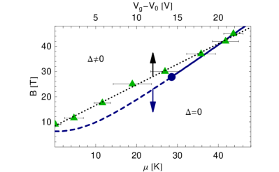
Figure 2: The upper line with triangles: The experimentally observed transition points between the lowest plateaus in the Hall conductivity from Ref. Zhang2006 . The lower line: The theoretical phase diagram in the plane of the magnetic field $B$ and the chemical potential $\mu$ for $\gamma=18$ K and $T=30$ mK. First and second order phase transitions are denoted by solid and dashed lines, respectively.

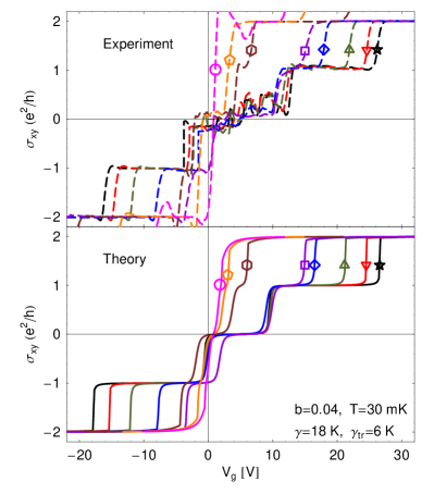
Figure 3: Hall conductivity in the experiment Zhang2006 (upper panel) and in the theoretical model (lower panel) for magnetic fields $B=9$ T (circle), $11.5$ T (pentagon), $17.5$ T (hexagon), $25$ T (square), $30$ T (diamond), $37$ T (up triangle), $42$ T (down triangle), and $45$ T (star). The parameters in the model are $b=0.04$, $\gamma=18$ K, $\gamma_{\rm tr}=6$ K, and temperature $T=30$ mK.

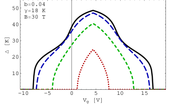
Figure 4: The gap $\Delta$ versus $V_{g}$ for $B=30$ T and four different values of temperature, $T=30$ mK, $5$ K, $10$ K, and $15$ K, from top to bottom.

In the rest of the paper, we will analyze the realistic case, with a spin splitting taken into account, whose dynamics is much richer. The thermodynamic potential $\Omega$, the Hall conductivity $\sigma_{xy}$ and the diagonal conductivity $\sigma_{xx}$ are now:

$$\Omega(\Delta,\mu)=\frac{1}{2}(\tilde{\Omega}(\Delta,\mu_{+})+\tilde{\Omega}(\Delta,\mu_{-})),$$ (10)

$$\sigma_{xy}=\frac{1}{2}(\tilde{\sigma}_{xy}(\mu_{+})+\tilde{\sigma}_{xy}(\mu_{-})),$$ (11)

$$\sigma_{xx}=\frac{1}{2}(\tilde{\sigma}_{xx}(\mu_{+})+\tilde{\sigma}_{xx}(\mu_{-})),$$ (12)

where the expressions for $\tilde{\Omega}$, $\tilde{\sigma}_{xy}$ and $\tilde{\sigma}_{xx}$ are given in Eqs. (3), (7), and (38) in Appendix B, respectively, and $\mu_{\pm}=\mu\pm\delta_{z}$, with $\delta_{z}=\mu_{B}B$ being the Zeeman term. This term breaks explicitly the $U(4)$ symmetry down to $U(2)_{c}\times U(2)_{d}$ discussed in Appendix C.

In order to determine the parameters of the theoretical model, we use the experimental data of Ref. Zhang2006 as a guide. In the regime when the excitonic gap is sufficiently large to remove the degeneracy of the LLL, the model predicts that one of the transition points between the plateaus in the Hall conductivity corresponds to a phase transition in which $\Delta\to 0$ (see the discussion connected with Fig. 4 below). More precisely, it is the transition point between the $\nu=0$ and $\nu=2$ plateaus for $B=11.5$ T, and the transition point between the $\nu=1$ and $\nu=2$ plateaus for larger values of $B$ (for $B=9$ T, with no plateau $\nu=0$, the transition point is taken to be zero). This is controlled by the value of the chemical potential $\mu$ (see Fig. 2). In the experiment, the corresponding control parameter is the gate voltage $V_{g}$. To obtain a relation between the two, we compare the theoretical phase diagram on the $B$–$\mu$ plane with the experimental phase diagram on the $B$–$V_{g}$ plane in Fig. 2. The latter is obtained by a simple compilation of the experimentally observed transition points between the corresponding plateaus in the Hall conductivity. The best fit that was found is:

$$\mu=0.5(V_{g}-V_{0})+7.0\,\mbox{sgn}(V_{g}-V_{0})\sqrt{|V_{g}-V_{0}|},$$ (13)

where while $\mu$ is measured in kelvins, $V_{g}$ is measured in volts, and $V_{0}$ is the center point in the dependence of the Hall conductivity obtained in experiment. Note that the values of $V_{0}$ are different for different values of $B$ and are in the interval from $0.8-5.8$ V footnote .

In Fig. 3, we present the experimental data for $\sigma_{xy}$ and their description in this model for the values of the parameters indicated in the figure. The form of the experimental and theoretical curves are quite similar. Note that the value of the parameter $b=0.04$ corresponds to a weak coupling with $g=e^{2}/\epsilon_{0}\hbar v_{F}\simeq 0.07$. Because of the three dimensional nature of the Coulomb interaction, it is plausible that the value of $g$ is influenced by a large dielectric constant $\epsilon_{0}$ of the substrate in the experimental device. The main reason of the necessity of a weak coupling for the fit is that the lengths of the experimental plateaus with $\nu=0,\pm 1,\pm 2$ imply that the Zeeman energy and the gap $\Delta$ are of the same order, and the Zeeman energy is only $\sim$ $10$ K at $B\sim 10$ T. Note that although there is no $\nu=0$ plateau in the $B=9$ T curve, the gap $\Delta$ in this case is also nonzero (although small). The reason is that in the presence of a nonzero scattering rate $\gamma$, the effect of a small gap, $\Delta\lesssim\gamma$, is unobservable.

In Fig. 4, the gap $\Delta$ versus $V_{g}$ for $B=30$ T and four different values of temperature is shown. At low $T=30$ mK, a strong first order phase transition with respect to $V_{g}$, i.e. $\mu$, is clearly seen. It corresponds to the transition point between the $\nu=\pm 1$ and $\nu=\pm 2$ plateaus. The steep descents, which occur approximately at the half of the critical value of $V_{g}-V_{0}$, are related to the transition between the $\nu=0$ and $\nu=\pm 1$ plateaus. The phase transition with respect to temperature is a second order one with the critical temperature $T_{c}\simeq 17.2$ K.

Fig. 1 in Introduction summarizes the main results of our analysis. Fig. 1d clearly shows that an excitonic gap $\Delta$ and a large enough Zeeman term ($\delta_{z}\gtrsim\gamma$) together lead to the QH plateaus with the filling factors $\nu=0,\pm 1$ and $\nu=\pm 2k$, $k=1,2,$…, i.e., those observed in Ref. Zhang2006 . Let us discuss this point in more detail. It is noticeable that while a large enough Zeeman term leads to the plateau $\nu=0$ even for $\Delta=0$ (see Figs. 1c), the $\nu=\pm 1$ plateaus appear only if both the Zeeman term is included and the gap $\Delta$ is nonvanishing (compare Fig. 1d with Figs. 1b and 1c). Therefore the $\nu=\pm 1$ plateaus are the clearest signature of the presence of a dynamical excitonic gap. There are of course also the plateaus $\nu=\pm 2$ connected with the LLL. As was already pointed out in Sec. II, the degeneracy of higher LLs is removed only by the Zeeman term (and not by the gap $\Delta$). Therefore the filling factors of the plateaus with $|\nu|>1$ are described by $\nu=\pm 2k$, $k=1,2,$….(see Fig. 1d) footnote3 . Thus, in this scenario, the LLL plays a very special role: While the excitonic gap does not reduce the degeneracy of higher LLs, it leads to splitting the LLL. This point is at heart of reproducing the QH effect data Zhang2006 in this scenario.

This picture is intimately connected with the removal of the degeneracy in this dynamics. As is shown in Appendix C, a nonzero $\Delta$ and the Zeeman term together break the initial non-abelian $U(4)$ symmetry down to the abelian $U(1)_{1}\times U(1)_{2}\times U(1)_{3}\times U(1)_{4}$ one. Since irreducible representations of abelian symmetries are one-dimensional, the $U(4)$ degeneracy of the LLL is completely removed.

By using Eqs. (12) and (38), we also checked that the values of $\Delta$ and $\gamma_{\rm tr}$ utilized in this section yield the diagonal conductivity $\sigma_{xx}$ whose behavior is in a qualitative agreement with the data in Ref. Zhang2006 .

IV Conclusion

We believe that the observation of the $\nu=0$ and $\nu=\pm 1$ plateaus in the experiment Zhang2006 strongly suggests that the existence of a dynamical excitonic gap (or gaps) in graphene in a strong magnetic field is a viable possibility. In this paper, only a singlet excitonic gap was considered. There of course exist other options: For example, the same Coulomb interaction can lead also to a nonzero triplet order parameter $\langle\bar{\Psi}\sigma^{3}\Psi\rangle$. In that case, the states with up and down spins will have different gaps, $\Delta_{+}$ and $\Delta_{-}$, respectively. The same arguments as those used above show that the degeneracy of higher LLs is lowered only by the Zeeman term and, therefore, in that case the filling factors of the the QH plateaus will be the same as in the case of the singlet excitonic gap. Therefore the modification of Fig. 1d will be only in replacing $\Delta$ with $\Delta_{\pm}$ for up and down spins.

In the present scenario, the weak coupling dynamics was utilized. The reason of its necessity is that the lengths of the experimental plateaus with $\nu=0,\pm 1,\pm 2$ imply that the Zeeman energy and the gap $\Delta$ are of the same order, and the Zeeman energy is only $\sim$ $10$ K at $B\sim 10$ T. Note, however, that this argument is valid only for a paramagnetic regime in which there is no large enhancement of spin splitting by dynamics in a magnetic field. When such a enhancement takes place Ferro1 , strong coupling dynamics might lead to a good fit of the experimental data in QH effect in graphene. This possibility will be considered elsewhere.

It is instructive to compare the present approach with other ones used for the description of the dynamics in QH effect in graphene. In Refs. Ferro2 ; Ferro3 , the QH ferromagnetism was considered. The main prediction in Ref. Ferro2 is that in this case the QH plateaus with all integer values of the filling factor $\nu$ occur [the critical values of a magnetic field $B$ at which plateaus occur are different for different $\nu$ and increase with $\nu$]. This prediction is quite different from the present one that reflects a difference between the dynamics in these two scenarios. As was emphasized above, the excitonic gap does not reduce the degeneracy of higher LLs and it is unlike the QH ferromagnetism. As a result, there are no odd filling factors $\nu=2k+1$, $k\geq 1$, in the scenario with excitonic gaps.

In Ref. Para , a scenario with the paramagnetic regime was considered (with no large enhancement of spin splitting). Unlike the present scenario, the breakdown of the $U(4)$ in Para is not spontaneous but explicit, provided by local (on-site) interactions. The main conclusion of Ref. Para is that Zeeman splitting together with on-site interactions can produce QH states at $\nu=0,\pm 1$ and $\pm 4$ but not at $\nu=\pm 3$ and $\pm 5$. Although the values of filling factors agree with ours, these two dynamics are very different and should lead to very different spectra of collective excitations.

Which of these scenarios is realized in graphene is an open issue. It would be interesting to include all possible competing orders in the thermodynamic potential and find the genuine ground state and the phase diagram in graphene Bascones2002PRL .

Appendix A Thermodynamic potential

In this Appendix we derive expression (3) for the thermodynamic potential per unit area $\tilde{\Omega}$ valid in the strong field limit, $\sqrt{\hbar v_{F}^{2}|eB|/c}\gg\gamma,T,\mu,\Delta$. We will use the formalism of the effective action introduced and developed in classical papers potential ; potential1 . In those papers, the case of the effective action for elementary fields was considered. The case of the effective action for local composite fields was studied in Ref. Miransky:1992bj and in our derivation we will follow that approach.

We start from a general definition of the effective action in a theory in which the spontaneous symmetry breaking phenomenon is driven by the local composite order parameter $\sigma=-\langle\bar{\Psi}\Psi\rangle\equiv-\langle 0|\bar{\Psi}\Psi|0\rangle$ corresponding to the generation of the excitonic gap $\Delta$ Khveshchenko2001PRL ; Gorbar2002PRB . Following the conventional way potential ; potential1 ; Miransky:1992bj , we introduce the generating functional $W(J)$ for the Green functions of the corresponding composite field through the path integral

$$e^{iW(J)}=\int D\Psi D\overline{\Psi}\exp\left\{i\int d^{3}x\left[{\cal L}_{qp}-J(x)\overline{\Psi}(x)\Psi(x)\right]\right\},$$ (14)

where $J(x)$ is the source for the composite field $-\bar{\Psi}(x)\Psi(x)$ and ${\cal L}_{qp}$ is the Lagrangian density of quasiparticles in the model at hand (note that here $x^{0}$ is the time variable $t$). Then, by definition, the effective action for the field $\sigma(x)=-\langle\overline{\Psi}(x)\Psi(x)\rangle$ is given by the Legendre transform of the generating functional $W(J)$,

$$\Gamma(\sigma)=W(J)-\int d^{3}xJ(x)\sigma(x),$$ (15)

where the external source $J(x)$ on the right-hand side is expressed in terms of the field $\sigma(x)$ by inverting the relation

$$\frac{\delta W(J)}{\delta J(x)}=\sigma(x).$$ (16)

The effective action $\Gamma(\sigma)$ in Eq. (15) provides a natural framework for describing the low energy dynamics in the model at hand. It is common to expand this action in powers of space-time derivatives of the field $\sigma$:

$$\Gamma(\sigma)=\int d^{3}x\left[-V(\sigma)+\frac{1}{2}Z^{\mu\nu}\partial_{\mu}\sigma\partial_{\nu}\sigma+\cdots\right],$$ (17)

where $V(\sigma)$ is the effective potential. The ellipsis denote higher derivative terms as well as contributions of the Nambu-Goldstone bosons. From Eqs. (15) and (16), we derive the following relation:

$$\frac{\delta\Gamma(\sigma)}{\delta\sigma(x)}=-J(x).$$ (18)

In the limit of a vanishing external source, this equation turns into an equation of motion for the composite field $\sigma(x)$. In a particular case of constant configurations, the equation reads $dV/d\sigma=0$.

The thermodynamic potential $\tilde{\Omega}$ per unit area in Eq. (3) is nothing else but the effective potential $V$ at non-zero $T$ and $\mu$. The constant source $J$ plays the role of the bare gap (Dirac mass), $J\equiv\Delta_{0}$. Then the initial relation in the derivation of $\tilde{\Omega}$ (following from Eqs. (17) and (18)) is:

$$\frac{\partial\tilde{\Omega}}{\partial\sigma}=\Delta_{0}.$$ (19)

At zero $T,\mu$ and $\gamma$, the gap equation with nonzero $\Delta_{0}$ in a strong field has the form (see Eq.(51) in Ref. Gorbar2002PRB ))

$$\Delta=\Delta_{0} + ie^{2}\int\frac{d\omega}{2\pi}\frac{\Delta}{\omega^{2}-\Delta^{2}}$$ (20)

$$\times \int\frac{d^{2}k}{(2\pi)^{2}}\exp\left[-\frac{\hbar c|\mathbf{k}|^{2}}{2|eB|}\right]U(\mathbf{k}),$$

where

$$U(\mathbf{k})=\frac{2\pi}{\epsilon_{0}}\frac{1}{|\mathbf{k}|(1+a|\mathbf{k}|)},\quad a=4\pi\nu_{0}\frac{e^{2}}{\epsilon_{0}\hbar v_{F}}\sqrt{\frac{\hbar c}{|eB|}},$$ (21)

and the const $\nu_{0}\approx 0.14$ (see Eqs. (46) and (47) in Gorbar2002PRB ). At finite T, $\mu$ and $\gamma$, the gap equation is written as the following sum over Matsubara frequencies $\omega_{n}=\pi T(2n+1)$:

$$\Delta=\Delta_{0}+2bL(B)T\sum\limits_{n=-\infty}^{\infty}\frac{\Delta}{(\omega_{n}+\gamma\,{\rm sgn}(\omega_{n})-i\mu)^{2}+\Delta^{2}}.$$ (22)

The sum over Matsubara frequencies is easily performed,

$$T\sum\limits_{n=-\infty}^{\infty}\frac{\Delta}{(\omega_{n}+\gamma\,{\rm sgn}(\omega_{n})-i\mu)^{2}+\Delta^{2}}$$

$$=\frac{1}{2\pi}{\rm Im}\left[\Psi\left(\frac{\gamma+i(\mu+\Delta)}{2\pi T}+\frac{1}{2}\right)-\left(\Delta\rightarrow-\Delta\right)\right],$$ (23)

where $\Psi$ is the digamma function. Then the gap equation takes the form

$$\Delta=\Delta_{0} + bL(B)\frac{1}{\pi}{\rm Im}\left[\Psi\left(\frac{\gamma+i(\mu+\Delta)}{2\pi T}+\frac{1}{2}\right)\right.$$ (24)

$$- \left.\Psi\left(\frac{\gamma+i(\mu-\Delta)}{2\pi T}+\frac{1}{2}\right)\right].$$

Let us express $\Delta_{0}$ through $\Delta$ from this equation and substitute it into Eq. (19). Then, taking into account the relation

$$\frac{\partial\tilde{\Omega}}{\partial\sigma}=\frac{\partial\tilde{\Omega}}{\partial\Delta}\cdot\frac{d\Delta}{d\sigma},$$ (25)

we come to the final equation

$$\frac{\partial\tilde{\Omega}}{\partial\Delta}=\frac{d\sigma}{d\Delta}\left[\Delta-bL(B)f(\Delta,\mu)\right],$$ (26)

where the function $f(\Delta,\mu)$ is given in Eq. (4). The condition $\partial\tilde{\Omega}/\partial\Delta=0$ yields gap equation (6) in the main text.

Since the field $\sigma=-\langle\overline{\Psi}\Psi\rangle$, we need to evaluate the chiral (excitonic) condensate which is given by

$$\langle\overline{\Psi}\Psi\rangle=-T\sum\limits_{n=-\infty}^{\infty}\int\frac{d^{2}k}{(2\pi)^{2}}\,{\rm tr}S(\omega_{n},k),$$ (27)

where the fermion propagator in the LLL is

$$S(\omega_{n},k)=2P_{-}e^{-k^{2}/|eB|}\frac{1}{\gamma_{0}(\omega_{n}+\gamma\,{\rm sgn}(\omega_{n})-i\mu)-\Delta}$$ (28)

with $P_{-}=(1-i\gamma^{1}\gamma^{2})/2$.

Calculating the trace and integrating over momenta we get

$$\langle\overline{\Psi}\Psi\rangle=-\frac{2|eB|T}{\pi}\sum\limits_{n=-\infty}^{\infty}\frac{\Delta}{(\omega_{n}+\gamma\,{\rm sgn}(\omega_{n})-i\mu)^{2}+\Delta^{2}}.$$ (29)

The sum over Matsubara frequencies is evaluated by means of Eq. (23) and we obtain

$$\sigma=-\langle\overline{\Psi}\Psi\rangle=\frac{1}{\pi l^{2}}f(\Delta,\mu).$$ (30)

Therefore Eq. (26) can be rewritten as

$$\frac{\partial\tilde{\Omega}}{\partial\Delta}=\frac{1}{\pi l^{2}}\frac{df(\Delta,\mu)}{d\Delta}\left[\Delta-bL(B)f(\Delta,\mu)\right].$$ (31)

Integrating over $\Delta$ we find

$$\tilde{\Omega}(\Delta,\mu)=\frac{1}{\pi l^{2}}\left\{\Delta f(\Delta,\mu)-\frac{bL(B)}{2}f^{2}(\Delta,\mu)\right.$$

$$\left.+{2T}{\rm Re}\left[\ln\Gamma\left(\frac{\gamma+i(\mu+\Delta)}{2\pi T}+\frac{1}{2}\right)\right.\right.$$

$$\left.\left.+\ln\Gamma\left(\frac{\gamma+i(\mu-\Delta)}{2\pi T}+\frac{1}{2}\right)\right]+C(\mu)\right\},$$ (32)

where the integration constant $C(\mu)$ was added on the right-hand side. Since $C(\mu)$ determines only the overall normalization of the potential, we can take it such that $\tilde{\Omega}(\Delta=0,\mu=0)=0$. As a result, we arrive at Eq. (3) in the main text. From Eq. (32) we also find that on the solution of the gap equation $\partial\tilde{\Omega}/\partial\Delta=0$, the carrier density $\rho$ is given by the expression

$$\frac{\partial\tilde{\Omega}}{\partial\mu}=-\rho=-\frac{1}{\pi l^{2}}\frac{1}{\pi}{\rm Im}\left[\Psi\left(\frac{\gamma+i(\mu+\Delta)}{2\pi T}+\frac{1}{2}\right)\right.$$

$$\left.+\Psi\left(\frac{\gamma+i(\mu-\Delta)}{2\pi T}+\frac{1}{2}\right)\right].$$ (33)

Appendix B Calculation of the conductivities

In the bare bubble approximation, the expression for the diagonal conductivity in the limit of $B\to\infty$ can be obtained from Eqs. (3.11), (3.12) in the second paper in Ref. Gusynin2005PRL ($\hbar=1$ in Appendix B)

$$\begin{split}\tilde{\sigma}_{xx}&=\frac{e^{2}\gamma_{\rm tr}}{\pi^{2}}\int\limits_{-\infty}^{\infty}\frac{d\omega}{4T\cosh^{2}\frac{\omega-\mu}{2T}}\\ &\left[\frac{\gamma_{\rm tr}}{\gamma_{\rm tr}^{2}+(\omega-\Delta)^{2}}+\frac{\gamma_{\rm tr}}{\gamma_{\rm tr}^{2}+(\omega+\Delta)^{2}}\right]\end{split}$$ (34)

[due to reasons pointed out in Sec. II, we use $\gamma_{\rm tr}$, and not $\gamma$, in conductivities $\sigma_{xx}$ and $\sigma_{xy}$]. The integrals in this expression can be evaluated exactly as follows. First we write

$$\begin{split}&I=\int\limits_{-\infty}^{\infty}\frac{d\omega}{\cosh^{2}\frac{\omega-\mu}{2T}}\frac{\gamma_{\rm tr}}{\gamma_{\rm tr}^{2}+(\omega-\Delta)^{2}}\\ &={\rm Re}\int\limits_{0}^{\infty}dt\,e^{-\gamma_{\rm tr}t}\int\limits_{-\infty}^{\infty}\frac{d\omega\,e^{it(\omega-\Delta)}}{\cosh^{2}\frac{\omega-\mu}{2T}}\\ &=2T{\rm Re}\int\limits_{0}^{\infty}dt\,e^{-t[\gamma_{\rm tr}-i(\mu-\Delta)]}\int\limits_{-\infty}^{\infty}\frac{dx}{\cosh^{2}x}\,e^{i2Ttx}\\ &=4T{\rm Re}\int\limits_{0}^{\infty}dt\,e^{-t[\gamma_{\rm tr}-i(\mu-\Delta)]}\int\limits_{0}^{\infty}\frac{dx\cos(2Ttx)}{\cosh^{2}x}.\end{split}$$ (35)

The integral over $x$ is evaluated by means of the formula (3.982.1) from Ref. Gradstein_Ryzhik . Then we get

$$I=4\pi T^{2}\int\limits_{0}^{\infty}\frac{dtt\cos[(\mu-\Delta)t]\,e^{-t\gamma_{\rm tr}}}{\sinh(\pi Tt)}.$$ (36)

This integral can be evaluated by differentiating Eq. (4.131.3) of Ref. Gradstein_Ryzhik which yields

$$\begin{split}&I=4\pi T^{2}\int\limits_{0}^{\infty}\frac{dtt\cos[(\mu-\Delta)t]\,e^{-t\gamma_{\rm tr}}}{\sinh(\pi Tt)}\\ &=\frac{2}{\pi}\,{\rm Re}\,\Psi^{\prime}\left(\frac{\gamma_{\rm tr}+i(\mu-\Delta)}{2\pi T}+\frac{1}{2}\right).\end{split}$$ (37)

Thus we obtain

$$\begin{split}\tilde{\sigma}_{xx}=&\frac{e^{2}\gamma_{\rm tr}}{2\pi^{3}T}\,{\rm Re}\left[\Psi^{\prime}\left(\frac{\gamma_{\rm tr}+i(\mu+\Delta)}{2\pi T}+\frac{1}{2}\right)\right.\\ &+\left.\Psi^{\prime}\left(\frac{\gamma_{\rm tr}+i(\mu-\Delta)}{2\pi T}+\frac{1}{2}\right)\right].\end{split}$$ (38)

One can check that for $\mu=0$ and $T\to 0$ Eq. (38) reduces to Eq. (9).

Now we derive the expression for the dc Hall conductivity. In the limit $B\to\infty$, Eqs. (3.14) and (3.15) in the second paper in Ref. Gusynin2005PRL yield

$$\begin{split}\tilde{\sigma}_{xy}&=-\frac{e^{2}{\rm sgn}(eB)}{4\pi^{2}T}\int\limits_{-\infty}^{\infty}\frac{d\omega}{\cosh^{2}\frac{\omega-\mu}{2T}}\\ &\times\left[\frac{\gamma_{\rm tr}(\omega-\Delta)}{\gamma_{\rm tr}^{2}+(\omega-\Delta)^{2}}+\frac{\gamma_{\rm tr}(\omega+\Delta)}{\gamma_{\rm tr}^{2}+(\omega+\Delta)^{2}}\right.\\ &\left.+\arctan\frac{\omega+\Delta}{\gamma_{\rm tr}}+\arctan\frac{\omega-\Delta}{\gamma_{\rm tr}}\right].\end{split}$$ (39)

We first consider the terms with $\arctan$ functions taking derivative with respect to $\Delta$:

$$\begin{split}\frac{d\tilde{\sigma}_{xy}^{(1)}}{d\Delta}&=-\frac{e^{2}{\rm sgn}(eB)}{4\pi^{2}T}\int\limits_{-\infty}^{\infty}\frac{d\omega}{\cosh^{2}\frac{\omega-\mu}{2T}}\\ &\times\left[\frac{\gamma_{\rm tr}}{\gamma_{\rm tr}^{2}+(\omega+\Delta)^{2}}-\frac{\gamma_{\rm tr}}{\gamma_{\rm tr}^{2}+(\omega-\Delta)^{2}}\right].\end{split}$$ (40)

Then we use Eq. (37) and find

$$\begin{split}\frac{d\tilde{\sigma}_{xy}^{(1)}}{d\Delta}=-&\frac{e^{2}{\rm sgn}(eB)}{2\pi^{3}T}\,{\rm Re}\left[\Psi^{\prime}\left(\frac{\gamma_{\rm tr}+i(\mu+\Delta)}{2\pi T}+\frac{1}{2}\right)\right.\\ &\left.-\Psi^{\prime}\left(\frac{\gamma_{\rm tr}+i(\mu-\Delta)}{2\pi T}+\frac{1}{2}\right)\right].\end{split}$$ (41)

Therefore

$$\begin{split}\tilde{\sigma}_{xy}^{(1)}=-&\frac{e^{2}{\rm sgn}(eB)}{\pi^{2}}\,{\rm Im}\left[\Psi\left(\frac{\gamma_{\rm tr}+i(\mu+\Delta)}{2\pi T}+\frac{1}{2}\right)\right.\\ &\left.+\Psi\left(\frac{\gamma_{\rm tr}+i(\mu-\Delta)}{2\pi T}+\frac{1}{2}\right)\right].\end{split}$$ (42)

Here we took into account the fact that because of the condition $\tilde{\sigma}_{xy}(\Delta=\infty)=0$ [see Eq. (39)] and the known asymptotics of the $\Psi$-function, the integration constant equals zero.

As to the integrals of the two first terms in square brackets in Eq. (39), they are calculated by means of the formula

$$\begin{split}&\int\limits_{-\infty}^{\infty}\frac{d\omega}{\cosh^{2}\frac{\omega-\mu}{2T}}\frac{\omega-\Delta}{\gamma_{\rm tr}^{2}+(\omega-\Delta)^{2}}\\ &=-\frac{2}{\pi}\,{\rm Im}\Psi^{\prime}\left(\frac{\gamma_{\rm tr}+i(\mu-\Delta)}{2\pi T}+\frac{1}{2}\right).\end{split}$$ (43)

Its derivation is as follows:

$$\begin{split}&\int\limits_{-\infty}^{\infty}\frac{d\omega}{\cosh^{2}\frac{\omega-\mu}{2T}}\frac{\omega-\Delta}{\gamma_{\rm tr}^{2}+(\omega-\Delta)^{2}}\\ &={\rm Re}\int\limits_{-\infty}^{\infty}\frac{d\omega}{\cosh^{2}\frac{\omega-\mu}{2T}}\frac{1}{\omega-\Delta+i\gamma_{\rm tr}}\\ &={\rm Im}\int\limits_{0}^{\infty}dt\,e^{-\gamma_{\rm tr}t}\int\limits_{-\infty}^{\infty}\frac{d\omega\,e^{it(\omega-\Delta)}}{\cosh^{2}\frac{\omega-\mu}{2T}}\\ &=2T{\rm Im}\int\limits_{0}^{\infty}dt\,e^{-t[\gamma_{\rm tr}-i(\mu-\Delta)]}\int\limits_{-\infty}^{\infty}\frac{dx}{\cosh^{2}x}\,e^{i2Ttx}\\ &=4T{\rm Im}\int\limits_{0}^{\infty}dt\,e^{-t[\gamma_{\rm tr}-i(\mu-\Delta)]}\int\limits_{0}^{\infty}\frac{dx\cos(2Ttx)}{\cosh^{2}x}\\ &=4\pi T^{2}\int\limits_{0}^{\infty}\frac{dtt\sin[(\mu-\Delta)t]\,e^{-t\gamma_{\rm tr}}}{\sinh(\pi Tt)}\\ &=-4\pi T^{2}\frac{d}{d\gamma_{\rm tr}}\int\limits_{0}^{\infty}\frac{dt\sin[(\mu-\Delta)t]\,e^{-t\gamma_{\rm tr}}}{\sinh(\pi Tt)}\\ &=-\frac{2}{\pi}{\rm Im}\Psi^{\prime}\left(\frac{\gamma_{\rm tr}+i(\mu-\Delta)}{2\pi T}+\frac{1}{2}\right),\end{split}$$ (44)

where, in the very last equality, Eq. (4.131.3) in Ref. Gradstein_Ryzhik was used. Combining this contribution with that in Eq. (42), we arrive at Eq. (II).

Appendix C $U(4)$ symmetry

The $U(4)$ symmetry in graphene is discussed for example in Appendix A in Ref. Gorbar2002PRB . Here we will describe the properties of this symmetry used in the main body of the paper.

The 16 generators of the $U(4)$ are

$$\frac{\sigma^{\alpha}}{2}\otimes I_{4},\quad\frac{\sigma^{\alpha}}{2i}\otimes\gamma^{3},\quad\frac{\sigma^{\alpha}}{2}\otimes\gamma^{5},\quad\mbox{and}\quad\frac{\sigma^{\alpha}}{2}\otimes\frac{1}{2}[\gamma^{3},\gamma^{5}],$$ (45)

where $I_{4}$ is the $4\times 4$ Dirac unit matrix and $\sigma^{\alpha}$, with $\alpha=0,1,2,3$, are four Pauli matrices connected with spin degrees of freedom [$\sigma^{0}$ is the $2\times 2$ unit matrix]. The Dirac matrices are connected with degrees of freedom reflecting the band structure of graphene with two inequivalent Dirac points at the corners of the Brillouin zone. In the representation used in the present paper (see Sec. II), the Dirac matrices $\gamma^{3}$ and $\gamma^{5}$ are:

$$\gamma^{3}=i\left(\begin{array}[]{cc}0&I\\ I&0\end{array}\right),\quad\gamma^{5}=i\left(\begin{array}[]{cc}0&I\\ -I&0\end{array}\right),$$ (46)

where $I$ is the $2\times 2$ unit matrix. The order parameter connected with the generation of the excitonic gap $\Delta$ is $\sigma=-\langle\overline{\Psi}\Psi\rangle\equiv-\langle\Psi^{\dagger}\gamma^{0}\Psi\rangle$ Gusynin1995PRD ; Khveshchenko2001PRL ; Gorbar2002PRB , where the Dirac matrix $\gamma^{0}$ anticommutes both with $\gamma^{3}$ and $\gamma^{5}$ and commutes with $[\gamma^{3},\gamma^{5}]$. The nonzero expectation value $\langle\overline{\Psi}\Psi\rangle=\langle[\psi_{KA\sigma}^{\dagger}\psi_{KA\sigma}+\psi_{K^{\prime}A\sigma}^{\dagger}\psi_{K^{\prime}A\sigma}-\psi_{KB\sigma}^{\dagger}\psi_{KB\sigma}-\psi_{K^{\prime}B\sigma}^{\dagger}\psi_{K^{\prime}B\sigma}]\rangle$ is directly related to the electron density imbalance between $A$ and $B$ sublattices of the bipartite hexagonal lattice of the graphene sheet Khveshchenko2001PRL ; Khveshchenko2004nb . The dynamical generation of the gap leads to the spontaneous breakdown of the $U(4)$ down to the $U(2)_{a}\times U(2)_{b}$ with the generators

$$\frac{\sigma^{\alpha}}{2}\otimes I_{4},\quad\frac{\sigma^{\alpha}}{2}\otimes\frac{1}{2}[\gamma^{3},\gamma^{5}]$$ (47)

[note that, as one can see from Eq. (46), $[\gamma^{3},\gamma^{5}]$ is diagonal]. As to the Zeeman term, it is connected with the spin density operator $\Psi^{\dagger}\sigma^{3}\Psi$. Therefore this term explicitly breaks the $U(4)$ down to the $U(2)_{c}\times U(2)_{d}$ with the generators

$$\frac{\sigma^{\alpha^{\prime}}}{2}\otimes I_{4},\quad\frac{\sigma^{\alpha^{\prime}}}{2i}\otimes\gamma^{3},\quad\frac{\sigma^{\alpha^{\prime}}}{2}\otimes\gamma^{5},\quad\mbox{and}\quad\frac{\sigma^{\alpha^{\prime}}}{2}\otimes\frac{1}{2}[\gamma^{3},\gamma^{5}],$$ (48)

where $\alpha^{\prime}=0,3$. Eqs. (47) and (48) imply that the Zeeman term and the generation of the gap together break the $U(4)$ down to the $U(1)_{1}\times U(1)_{2}\times U(1)_{3}\times U(1)_{4}$ with the four diagonal generators

$$\frac{\sigma^{\alpha^{\prime}}}{2}\otimes I_{4}\,,\quad\frac{\sigma^{\alpha^{\prime}}}{2}\otimes\frac{1}{2}[\gamma^{3},\gamma^{5}]\,;\quad\alpha^{\prime}=0,3.$$ (49)

References

- (1) K.S. Novoselov, A.K. Geim, S.V. Morozov, D. Jiang, Y. Zhang, S.V. Dubonos, I.V. Grigorieva, and A.A. Firsov, Science 306, 666 (2004).
- (2) K.S. Novoselov, A.K. Geim, S.V. Morozov, D. Jiang, M.I. Katsnelson, I.V. Grigorieva, S.V. Dubonos,and A.A. Firsov, Nature 438, 197 (2005).
- (3) Y. Zhang, Y.-W. Tan, H.L. Störmer, and P. Kim, Nature 438, 201 (2005).
- (4) V.P. Gusynin and S.G. Sharapov, Phys. Rev. Lett. 95, 146801 (2005); V.P. Gusynin and S.G. Sharapov, Phys. Rev. B 73, 245411 (2006).
- (5) N.M.R. Peres, F. Guinea, and A.H. Castro Neto, Phys. Rev. B 73, 1254111 (2006).
- (6) D. M. Haldane, Phys. Rev. Lett. 61, 2015 (1988); Y. Zheng and T. Ando, Phys. Rev. B 65, 245420 (2002).
- (7) G.W. Semenoff, Phys. Rev. Lett. 53, 2449 (1984).
- (8) Y. Zhang, Z. Jiang, J.P. Small, M.S. Purewal, Y.-W. Tan, M. Fazlollahi, J.D. Chudow, J.A. Jaszczak, H.L. Stormer, P. Kim, Phys. Rev. Lett. 96, 136806 (2006).
- (9) A possibility of a scenario with a strong coupling dynamics is discussed in Sec. IV.
- (10) V.P. Gusynin, V.A. Miransky, and I.A. Shovkovy, Phys. Rev. Lett. 73, 3499 (1994); Phys. Rev. D 52, 4718 (1995); Nucl. Phys. B 462, 249 (1996).
- (11) The crucial feature underlying the magnetic catalysis phenomenon is the presence of the LLL with energy containing both electron and hole states. This property of graphene distinguishes it from inversion layers.
- (12) D.V. Khveshchenko, Phys. Rev. Lett. 87, 206401 (2001); ibid. 87, 246802 (2001).
- (13) E.V. Gorbar, V.P. Gusynin, V.A. Miransky, and I.A. Shovkovy, Phys. Rev. B 66, 045108 (2002).
- (14) Y. Kopelevich, V. V. Lemanov, S. Moehlecke, and J. H. S. Torres, Fiz. Tverd. Tela 41, 2135 (1999) [Phys. Solid State 41, 1959 (1999)]; H. Kempa, Y. Kopelevich, F. Mrowka, A. Setzer, J. H. S. Torres, R. Höhne, and P. Esquinazi, Solid State Commun. 115, 539 (2000); M. S. Sercheli, Y. Kopelevich, R. R. da Silva, J. H. S. Torres, and C. Rettori, Solid State Commun. 121, 579 (2002). For the latest results of this group, see Y. Kopelevich, J. C. Medina Pantoja, R. R. da Silva, F. Mrowka, and P. Esquinazi, Phys. Lett. A 355, 233 (2006).
- (15) E.V. Gorbar, V.P. Gusynin, V.A. Miransky, and I.A. Shovkovy, Phys. Lett. A 313, 472 (2003).
- (16) H. Leal and D.V. Khveshchenko, Nucl. Phys. B 687, 323 (2004); D.V. Khveshchenko and W.F. Shively, Phys. Rev. B 73, 115104 (2006).
- (17) V. A. Miransky, Int. J. Mod. Phys. A 8, 135 (1993).
- (18) V.P. Gusynin, S. G. Sharapov and J. P. Carbotte, Phys. Rev. Lett. 96, 256802 (2006).
- (19) T. Ando, J. Phys. Soc. Jpn. 74, 777 (2005).
- (20) Because of a nonzero scattering rate , the effect of a small gap, , is unobservable and, therefore, the location of the transitions between the plateaus are not expected to coincide exactly with the point where vanishes. This leads to uncertainties in the relation between the theoretical model parameter and the experimental quantity . We use the results in Fig. 2 only to find a qualitatively reasonable relation between them.
- (21) In fact, as was shown above, the gap disappears for the values of the chemical potential corresponding to higher LLs in this dynamics (see Fig. 4). Therefore the fact that the degeneracy of higher LLs is removed only by the Zeeman term in this case is evident.
- (22) A regime with a strong enhancement of spin splitting by electron exchange interaction in graphene was considered in D.A. Abanin, P.A. Lee, and L.S. Levitov, Phys. Rev. Lett. 96, 176803 (2006). It was pointed out that in this case spin splitting should lead to a large gap of order 100 K producing a QH plateau with .
- (23) K. Nomura and A. H. MacDonald, Phys. Rev. Lett. 96, 256602 (2006).
- (24) M.O. Goerbig, R. Moessner, and B. Doucot, Phys. Rev. B 74, 161407(R) (2006).
- (25) J. Alicea and M.P.A. Fisher, Phys. Rev. B 74, 075422 (2006).
- (26) An early study of a doped excitonic insulator with the quadratic quasiparticle dispersion law in dimensions in E. Bascones, A. A. Burkov, and A. H. MacDonald, Phys. Rev. Lett. 89, 086401 (2002) revealed a very rich phase diagram.
- (27) J. Goldstone, A. Salam, and S. Weinberg, Phys. Rev. 127, 962 (1962); G. Jona-Lasinio, Nuovo Cimento 34, 1790 (1964).
- (28) S. R. Coleman and E. Weinberg, Phys. Rev. D 7, 1888 (1973); L. Dolan and R. Jackiw, Phys. Rev. D 9, 3320 (1974).
- (29) I. S. Gradshtein and I. M. Ryzhik, Table of Integrals, Series and Products (Academic Press, Orlando, 1994).