How ‘sticky’ are short-range square-well fluids?

Abstract

The aim of this work is to investigate to what extent the structural properties of a short-range square-well (SW) fluid of range $\lambda$ at a given packing fraction $\eta$ and reduced temperature $T^{*}=k_{B}T/\epsilon$ can be represented by those of a sticky-hard-sphere (SHS) fluid at the same packing fraction and an effective stickiness parameter $\tau(T^{*},\lambda)$. Such an equivalence cannot hold for the radial distribution function $g(r)$ since this function has a delta singularity at contact ($r=\sigma$) in the SHS case, while it has a jump discontinuity at $r=\lambda\sigma$ in the SW case. Therefore, the equivalence is explored with the cavity function $y(r)$, i.e., we assume that $y_{\text{SW}}(r|\eta,T^{*};\lambda)\approx y_{\text{SHS}}(r|\eta,\tau(T^{*},\lambda))$. Optimization of the agreement between $y_{\text{SW}}$ and $y_{\text{SHS}}$ to first order in density suggests the choice $\tau(T^{*},\lambda)=[12({e}^{1/T^{*}}-1)(\lambda-1)]^{-1}$. We have performed Monte Carlo (MC) simulations of the SW fluid for $\lambda=1.05$, $1.02$, and $1.01$ at several densities and temperatures $T^{*}$ such that $\tau(T^{*},\lambda)=0.13$, $0.2$, and $0.5$. The resulting cavity functions have been compared with MC data of SHS fluids obtained by Miller and Frenkel [J. Phys: Cond. Matter 16, S4901 (2004)]. Although, at given values of $\eta$ and $\tau$, some local discrepancies between $y_{\text{SW}}$ and $y_{\text{SHS}}$ exist (especially for $\lambda=1.05$), the SW data converge smoothly toward the SHS values as $\lambda-1$ decreases. In fact, precursors of the singularities of $y_{\text{SHS}}$ at certain distances due to geometrical arrangements are clearly observed in $y_{\text{SW}}$. The approximate mapping $y_{\text{SW}}\to y_{\text{SHS}}$ is exploited to estimate the internal energy and structure factor of the SW fluid from those of the SHS fluid. Taking for $y_{\text{SHS}}$ the solution of the Percus–Yevick equation as well as the rational-function approximation, the radial distribution function $g(r)$ of the SW fluid is theoretically estimated and a good agreement with our MC simulations is found. Finally, a similar study is carried out for short-range SW fluid mixtures.

I Introduction

It is well known that colloidal particles in a suspension of free polymers interact through effective attractive forces (of entropic origin) with a range and strength determined by the size and concentration of the polymers.HSKGKQ84 ; KRBDVM89 A simple model describing this effective interaction is the square-well (SW) potential

$$\varphi_{\text{SW}}(r)=\begin{cases}\infty,&r<\sigma,\\ -\epsilon,&\sigma<r<\lambda\sigma,\\ 0,&r>\lambda\sigma,\end{cases}$$ (1)

which accounts for excluded volume effects associated with the hard-core diameter $\sigma$ plus an attractive layer of relative width $\lambda-1$ and strength $\epsilon$. Although the SW potential (with $\lambda\simeq 1.5$) was originally introduced as a simple model for normal liquids,BH76 it has become even more useful in colloidal systems, where one typically has $\lambda\leq 1.1$.

The interaction parameters $\sigma$ and $\epsilon$ can be used to define the length and energy units, respectively. Thus, the concentration of particles can be characterized by the volume fraction $\eta=\frac{\pi}{6}\rho\sigma^{3}$, where $\rho$ is the number density, and the temperature $T$ can be measured in units of $\epsilon$ as $T^{*}=k_{B}T/\epsilon$, where $k_{B}$ is the Boltzmann constant. Therefore, at given $\eta$ and $T^{*}$, only the range $\lambda$ remains as a free parameter. This degree of freedom disappears in the so-called sticky-hard-sphere (SHS) limit,B68 where one takes the combined limits $\epsilon\to\infty$ (i.e., $T^{*}\to 0$) and $\lambda\to 1$, while keeping constant the stickiness parameter

$$\tau^{-1}=12{{e}^{1/T^{*}}}{(\lambda-1)}.$$ (2)

The parameter $\tau$ plays in the SHS fluid a role equivalent to that played by the reduced temperature $T^{*}$ in the SW fluid. Although, strictly speaking, a monodisperse system of SHS is not thermodynamically stable, a small degree of polydispersity is sufficient to restore stability.S91 Given its simplicity and the fact that it can be exactly solved within the Percus–Yevick (PY) approximation,B68 ; PS75 the SHS model has received considerable attention as a convenient model of colloidal suspensions.BT79 ; SG87 ; KF88 ; RR89 ; JBH91 ; MMR91 ; TB93 ; YS93a ; YS93b ; RAH95 ; TKR02 ; GG02 ; MF03 ; GG04 ; MF04a ; MF04b ; FGG05 ; J06

It is obvious that the thermodynamic and structural properties of the SW fluid must approach those of the SHS fluid as $\lambda\to 1$ at fixed $\eta$ and $\tau$. This has been tested, for instance, in the case of the vapour-liquid critical point.MF04a An interesting problem not yet addressed in detail is the rate of the convergence from SW to SHS. In other words, how small must the width $\lambda-1$ be for the properties of the SW system to be practically the same as those of an equivalent SHS system? Comparison between Monte Carlo (MC) simulationsHSKGKQ84 for an SW fluid with $\lambda=1.1$ and theoretical results for SHS fluids shows a good agreement between the respective structure factors $S(k)$,MMR91 ; YS94 ; AS01 although a systematic phase shift between both structure factors exists. This is a reflection of the fact that the radial distribution function $g(r)$, which is essentially the inverse Fourier transform of $S(k)$, has important qualitative differences in both classes of systems. While in the case of an SW fluid, $g(r)$ is finite at $r=\sigma^{+}$ and presents a jump discontinuity at $r=\lambda\sigma$, a delta-peak singularity at $r=\sigma^{+}$, followed by other delta and jump singularities at certain characteristic distances,SG87 ; MF04a appear in the SHS case.

The aim of this paper is two-fold. First, we want to assess to what degree a short-range SW fluid behaves as a suitably chosen “equivalent” SHS fluid. To that end, we have performed Monte Carlo (MC) simulations of SW systems with $\lambda=1.05$, $\lambda=1.02$, and $\lambda=1.01$, and have compared their structural properties with recent MC simulationsMF04a for SHS fluids at the same packing fraction and effective stickiness. The comparison is not carried out with the radial distribution function $g(r)$, but with the much more regular cavity (or background) function $y(r)={e}^{\varphi(r)/k_{B}T}g(r)$. It is observed that, as expected, the SW cavity functions converge toward the SHS ones as $\lambda$ decreases. However, the results show that the range $\lambda=1.05$ cannot be considered small enough to get a cavity function hardly distinguishable from the SHS one. The second point we address is the estimate of the structure factor and thermodynamic properties of short-range SW fluids from the knowledge of the properties of SHS fluids. As said before, the starting point is the assumption that both cavity functions are approximately the same. The approximate estimates for the internal energy and structure factor of the SW systems are tested against actual MC simulations, finding a good agreement. Also in this context, we take advantage of the exact solution of the PY equation for SHS,B68 as well as of a more refined theory,YS93b to propose analytic approximations for the radial distribution function of SW fluids. A parallel study is carried out for short-range SW fluid mixtures. Due to the scarcity of simulation results for SHS mixtures, we compare our MC results with the solution of the PY theory.PS75 It is observed that in the case of mixtures the influence of $\lambda\neq 1$ on the mapping SW$\to$SHS is similar to that in the one-component case.

This paper is organized as follows. The basic equations for SW and SHS fluids are summarized in Section II. The criterion followed in this paper to define the effective stickiness parameter and some consequences are elaborated in Section III. Section IV presents the comparison between our MC simulations for SW and those reported in Ref. MF04a, for SHS, while the comparison with theoretical predictions is presented in Section V. The case of SW mixtures is considered in Section VI. Finally, the paper ends with some concluding remarks.

II Basic equations

In this Section we introduce the notation and display the basic equations that will be needed in the paper.

II.1 The square-well fluid

The SW interaction potential is given by Eq. (1). Henceforth, the distance $r$ is assumed to be measured in units of the hard-core diameter $\sigma$, so that we take $\sigma=1$. The relevant physical information about the system is contained in the radial distribution function $g_{\text{SW}}(r|\eta,T^{*};\lambda)$, where the notation emphasizes that it depends on the thermodynamic state (characterized by the packing fraction $\eta$ and the reduced temperature $T^{*}$) and on the relative range $\lambda$. The corresponding cavity function is $y_{\text{SW}}(r|\eta,T^{*};\lambda)={e}^{\varphi_{\text{SW}}(r)/k_{B}T}g_{\text{SW}}(r|\eta,T^{*};\lambda)$. Inverting this relationship, one has

$$g_{\text{SW}}(r|\eta,T^{*};\lambda)=\begin{cases}0,&r<1,\\ {e}^{1/T^{*}}y_{\text{SW}}(r|\eta,T^{*};\lambda),&1<r<\lambda,\\ y_{\text{SW}}(r|\eta,T^{*};\lambda),&r>\lambda.\end{cases}$$ (3)

Since the cavity function is continuous everywhere,HM86 Eq. (3) implies that the radial distribution is discontinuous not only at $r=1$, but also at $r=\lambda$, namely $g_{\text{SW}}(\lambda^{-}|\eta,T^{*};\lambda)/g_{\text{SW}}(\lambda^{+}|\eta,T^{*};\lambda)={e}^{1/T^{*}}$.

The structure factor is defined as $S(k)=1+\rho\widetilde{h}(k)$, where $\widetilde{h}(k)$ is the Fourier transform of the total correlation function $h(r)\equiv g(r)-1$. In the case of the SW fluid, $S(k)$ can be obtained from $y(r)$ as

$$S_{\text{SW}}(k|\eta,T^{*};\lambda) = 1+\frac{24\eta}{k}\int_{0}^{\infty}{d}r\,r\sin kr\left[g_{\text{SW}}(r|\eta,T^{*};\lambda)-1\right]$$ (4)

$$= 1+\frac{24\eta}{k}\left\{-\int_{0}^{1}{d}r\,r{\sin kr}+({e}^{1/T^{*}}-1)\int_{1}^{\lambda}{d}r\,r{\sin kr}\,y_{\text{SW}}(r|\eta,T^{*};\lambda)\right.$$

$$\left.+\int_{1}^{\infty}{d}r\,r{\sin kr}\left[y_{\text{SW}}(r|\eta,T^{*};\lambda)-1\right]\right\}.$$

The thermodynamic properties can also be expressed in terms of the cavity function. The virial equation yields

$$Z_{\text{SW}}(\eta,T^{*};\lambda) = 1-\frac{4\eta}{k_{B}T}\int_{0}^{\infty}{d}r\,r^{3}g_{\text{SW}}(r|\eta,T^{*};\lambda)\frac{d}{dr}\varphi_{\text{SW}}(r)$$ (5)

$$= 1+4\eta\left[{e}^{1/T^{*}}y_{\text{SW}}(1|\eta,T^{*};\lambda)-({e}^{1/T^{*}}-1)\lambda^{3}y_{\text{SW}}(\lambda|\eta,T^{*};\lambda)\right],$$

where $Z\equiv p/\rho k_{B}T$ is the compressibility factor, $p$ being the pressure. The compressibility equation gives

$$\chi_{\text{SW}}(\eta,T^{*};\lambda) = S_{\text{SW}}(0|\eta,T^{*};\lambda)$$ (6)

$$= 1+{24\eta}\left\{({e}^{1/T^{*}}-1)\int_{1}^{\lambda}{d}r\,r^{2}y_{\text{SW}}(r|\eta,T^{*};\lambda)+\int_{1}^{\infty}{d}r\,r^{2}\left[y_{\text{SW}}(r|\eta,T^{*};\lambda)-1\right]-\frac{1}{3}\right\},$$

where $\chi\equiv k_{B}T(\partial\rho/\partial p)_{T}$ is the isothermal susceptibility. Finally, the excess internal energy per particle $u$ is

$$\frac{1}{\epsilon}u_{\text{SW}}(\eta,T^{*};\lambda) = \frac{\rho}{2\epsilon}\int{d}\mathbf{r}\,\varphi_{\text{SW}}(r)g_{\text{SW}}(r|\eta,T^{*};\lambda)$$

$$= -12\eta{e}^{1/T^{*}}\int_{1}^{\lambda}{d}r\,r^{2}y_{\text{SW}}(r|\eta,T^{*};\lambda).$$

Therefore, $-2u_{\text{SW}}/\epsilon$ coincides with the coordination number.

II.2 The sticky-hard-sphere limit

The SHS system can be obtained from the SW one by formally taking the combined limits $\lambda\to 1$ and $T^{*}\to 0$ with the stickiness parameter (2) kept constant:

$$y_{\text{SHS}}(r|\eta,\tau)=\lim_{T^{*}\to 0,\lambda\to 1}y_{\text{SW}}(r|\eta,T^{*};\lambda).$$ (8)

Equation (3) then reduces to

$$g_{\text{SHS}}(r|\eta,\tau)=\left[\frac{1}{12\tau}\delta(r-1)+\Theta(r-1)\right]y_{\text{SHS}}(r|\eta,\tau),$$ (9)

so that the radial distribution function becomes identical to the cavity function for $r>1$, but a delta-peak of amplitude proportional to the stickiness appears at contact.

In the SHS limit, Eqs. (4)–(II.1) become

$$S_{\text{SHS}}(k|\eta,\tau)=1+\frac{24\eta}{k}\left\{-\int_{0}^{1}{d}r\,r{\sin kr}+\frac{\sin k}{12\tau}y_{\text{SHS}}(1|\eta,\tau)+\int_{1}^{\infty}{d}r\,r{\sin kr}\left[y_{\text{SHS}}(r|\eta,\tau)-1\right]\right\},$$ (10)

$$Z_{\text{SHS}}(\eta,\tau)=1+4\eta\left[\left(1-\frac{1}{4\tau}\right)y_{\text{SHS}}(1|\eta,\tau)-\frac{1}{12\tau}y^{\prime}_{\text{SHS}}(1|\eta,\tau)\right]$$ (11)

$$\chi_{\text{SHS}}(\eta,\tau)=1+{24\eta}\left\{\frac{1}{12\tau}y_{\text{SHS}}(1|\eta,\tau)+\int_{1}^{\infty}{d}r\,r^{2}\left[y_{\text{SHS}}(r|\eta,\tau)-1\right]-\frac{1}{3}\right\},$$ (12)

$$\frac{1}{\epsilon}u_{\text{SHS}}(\eta,\tau)=-\frac{\eta}{\tau}y_{\text{SHS}}(1|\eta,\tau).$$ (13)

In Eq. (11), $y^{\prime}(r)$ denotes the first derivative of $y(r)$.

III Effective “stickiness”

Now we assume an SW fluid with a small, but non-zero, value of the well width $\lambda-1$. It is natural to expect that its structural properties are, at least to some extent, close to those of an SHS fluid characterized by suitably chosen effective packing fraction $\eta_{\text{eff}}$ and effective stickiness $\tau_{\text{eff}}^{-1}$. Comparison between Eqs. (3) and (9) shows that the radial distribution function $g(r)$ is not the adequate quantity to establish the approximate mapping SW$\to$SHS. This also applies to the structure factor $S(k)$ since it is essentially the Fourier counterpart of $g(r)$. Therefore, we choose the cavity function $y(r)$, which is a more regular function than $g(r)$. Thus, we consider here the approximation

$$y_{\text{SW}}(r|\eta,T^{*};\lambda)\approx y_{\text{SHS}}(r|\eta_{\text{eff}}(\eta,T^{*};\lambda),\tau_{\text{eff}}(\eta,T^{*};\lambda)).$$ (14)

Note that this implies $g_{\text{SW}}(r|\eta,T^{*};\lambda)\neq g_{\text{SHS}}(r|\eta_{\text{eff}}(\eta,T^{*};\lambda),\tau_{\text{eff}}(\eta,T^{*};\lambda))$ and $S_{\text{SW}}(k|\eta,T^{*};\lambda)\neq S_{\text{SHS}}(k|\eta_{\text{eff}}(\eta,T^{*};\lambda),\tau_{\text{eff}}(\eta,T^{*};\lambda))$. The next step consists of defining criteria to determine the effective quantities $\eta_{\text{eff}}(\eta,T^{*};\lambda)$ and $\tau_{\text{eff}}(\eta,T^{*};\lambda))$. There exist some obvious constraints. First, one must recover the hard-sphere (HS) cavity function from $y_{\text{SW}}$ if either $\lambda\to 1$ at fixed $T^{*}$ or $T^{*}\to\infty$ at fixed $\lambda$. More explicitly,

$$\lim_{\lambda\to 1}y_{\text{SW}}(r|\eta,T^{*};\lambda)=y_{\text{HS}}(r|\eta),$$ (15)

$$\lim_{T^{*}\to\infty}y_{\text{SW}}(r|\eta,T^{*};\lambda)=y_{\text{HS}}(r|\eta),$$ (16)

$$\lim_{\tau\to\infty}y_{\text{SHS}}(r|\eta,\tau)=y_{\text{HS}}(r|\eta).$$ (17)

This implies that

$$\lim_{\lambda\to 1}\eta_{\text{eff}}(\eta,T^{*};\lambda)=\eta,\quad\lim_{\lambda\to 1}\tau_{\text{eff}}(\eta,T^{*};\lambda)=\infty,$$ (18)

$$\lim_{T^{*}\to\infty}\eta_{\text{eff}}(\eta,T^{*};\lambda)=\eta,\quad\lim_{T^{*}\to\infty}\tau_{\text{eff}}(\eta,T^{*};\lambda)=\infty.$$ (19)

Moreover, Eq. (14) must become exact if the SHS limit is taken on the left-hand side and Eq. (8) is applied. Thus,

$$\lim_{T^{*}\to 0,\lambda\to 1}12(\lambda-1){e}^{1/T^{*}}\tau_{\text{eff}}(\eta,T^{*};\lambda)=1.$$ (20)

As is usual,KRBDVM89 ; SG87 ; RR89 ; MMR91 ; TB93 ; MF04a ; VL00 let us assume for simplicity that $\eta_{\text{eff}}(\eta,T^{*};\lambda)=\eta_{\text{eff}}(\eta,\lambda)$ is independent of temperature and $\tau_{\text{eff}}(\eta,T^{*};\lambda)=\tau_{\text{eff}}(T^{*};\lambda)$ is independent of density. The first choice allows us to determine $\eta_{\text{eff}}$ by applying the first equality of (19), which holds regardless of the value of $\lambda\geq 1$. It is then obvious that

$$\eta_{\text{eff}}(\eta,\lambda)=\eta.$$ (21)

On the other hand, the choice $\eta_{\text{eff}}(\eta,\lambda)=\eta\lambda^{3}$ adopted by Menon et al.MMR91 is in conflict with the HS limit (19).

In order to determine $\tau_{\text{eff}}(T^{*},\lambda)$, several criteria can be used. The conventional oneSG87 ; RR89 ; TB93 ; VL00 is to impose that the second virial coefficient of the SW fluid be the same as that of the SHS fluid, i.e., $B_{2}^{\text{SW}}(T^{*};\lambda)=B_{2}^{\text{SHS}}(\tau_{\text{eff}}(T^{*},\lambda))$. This yields

$$\tau_{\text{eff}}(T^{*},\lambda)=\frac{1}{12({e}^{1/T^{*}}-1)\alpha(\lambda)}$$ (22)

with $\alpha(\lambda)=\alpha_{3}(\lambda)$, where

$$\alpha_{n}(\lambda)\equiv\frac{1}{n}(\lambda^{n}-1).$$ (23)

The form (22) with $\alpha(\lambda)=\alpha_{n}(\lambda)$ is consistent with the constraints (18)–(20), regardless of the value of $n$. Since in the second virial coefficient one simply makes use of the zero-density cavity function $y(r)\to 1$, the choice $\alpha(\lambda)=\alpha_{3}(\lambda)$ is not necessarily the most efficient one from the point of view of Eq. (14) at finite density. Another common choiceMMR91 ; MF04a is $\tau_{\text{eff}}(T^{*},\lambda)={e}^{-1/T^{*}}/12(1-\lambda^{-1})$, but it is inconsistent with the HS constraint (19). The same happens with the direct extrapolation of (2) at finite $T^{*}$, i.e., $\tau_{\text{eff}}(T^{*},\lambda)={e}^{-1/T^{*}}/12(\lambda-1)$.

As a guide to choose $\tau_{\text{eff}}(T^{*},\lambda)$, let us resort to the exact cavity function to first order in density.BH67 In that case one has

$$y_{\text{SW}}(r|\eta,T^{*};\lambda)=1+y_{\text{SW}}^{(1)}(r|T^{*};\lambda)\eta+\mathcal{O}(\eta^{2}),$$ (24)

$$y_{\text{SHS}}(r|\eta,\tau)=1+y_{\text{SHS}}^{(1)}(r|\tau)\eta+\mathcal{O}(\eta^{2}),$$ (25)

where the expressions of $y_{\text{SW}}^{(1)}(r|T^{*};\lambda)$ and $y_{\text{SHS}}^{(1)}(r|\tau)$ are given in the Appendix. Comparison between both functions suggests to keep Eq. (22), except that it remains to determine $\alpha(\lambda)$ subject to the constraint $\lim_{\lambda\to 1}\alpha(\lambda)/(\lambda-1)=1$. In the region $1<r<2$ we have

$$y_{\text{SW}}^{(1)}(r|T^{*};\lambda) = 8-6r+\frac{1}{2}r^{3}$$ (26)

$$+\frac{3(\lambda^{2}-1)^{2}r^{-1}-8(\lambda^{3}-1)+6(\lambda^{2}-1)r}{12\tau_{\text{eff}}(T^{*},\lambda)\alpha(\lambda)}$$

$$+\frac{3(\lambda^{2}-1)^{2}r^{-1}}{[12\tau_{\text{eff}}(T^{*},\lambda)\alpha(\lambda)]^{2}},$$

$$y_{\text{SHS}}^{(1)}(r|\tau)=8-6r+\frac{1}{2}r^{3}+\frac{r-2}{\tau}+\frac{r^{-1}}{12\tau^{2}}.$$ (27)

It is clear that no unique choice of $\alpha(\lambda)$ can make $y_{\text{SW}}^{(1)}(r|T^{*};\lambda)=y_{\text{SHS}}^{(1)}(r|\tau_{\text{eff}}(T^{*},\lambda))$ for arbitrary $r$, $T^{*}$, and $\lambda$. In the limit of very low temperatures ($T^{*}\to 0\Rightarrow\tau_{\text{eff}}\to 0$) the respective last terms on the right-hand sides of Eqs. (26) and (27) dominate, so that $y_{\text{SW}}^{(1)}(r|T^{*};\lambda)\to y_{\text{SHS}}^{(1)}(r|\tau_{\text{eff}}(T^{*},\lambda))$ provided that one takes $\alpha(\lambda)=\alpha_{2}(\lambda)$, where $\alpha_{n}(\lambda)$ is defined by Eq. (23). Nevertheless, for temperatures such that $12\tau_{\text{eff}}\sim 1$, all the terms in Eqs. (26) and (27) are of the same order, so that again $\alpha(\lambda)=\alpha_{2}(\lambda)$ might not be the best choice. Restricting ourselves, for the sake of simplicity, to functions $\alpha(\lambda)$ of the form (23) with $n=\text{integer}$, it turns out that the optimal choice is generally $\alpha(\lambda)=\alpha_{1}(\lambda)$ for temperatures close to the critical one, i.e., if $\tau_{\text{eff}}\approx 0.1$.MF04b This is illustrated in Fig. 1 for the case $\lambda=1.05$ and $T^{*}=0.35$. While the choice $\alpha(\lambda)=\alpha_{2}(\lambda)=\frac{1}{2}(\lambda^{2}-1)$ gives a value of $y_{\text{SHS}}^{(1)}$ in excellent agreement with $y_{\text{SW}}^{(1)}$ at $r=1$, the best global agreement is provided by the choice $\alpha(\lambda)=\alpha_{1}(\lambda)=\lambda-1$. For larger temperatures the optimal choice could change to $\alpha(\lambda)=\alpha_{0}(\lambda)=\ln\lambda$ or even $\alpha(\lambda)=\alpha_{-1}(\lambda)=1-\lambda^{-1}$. Since we want to keep $\alpha(\lambda)$ independent of temperature, in what follows we adopt the choice $\alpha(\lambda)=\alpha_{1}(\lambda)$ for simplicity and also to enhance the cases with $\tau_{\text{eff}}\approx 0.1$. In summary, the definition of the effective stickiness parameter is taken as

$$\tau_{\text{eff}}(T^{*},\lambda)=\frac{1}{12({e}^{1/T^{*}}-1)(\lambda-1)}.$$ (28)

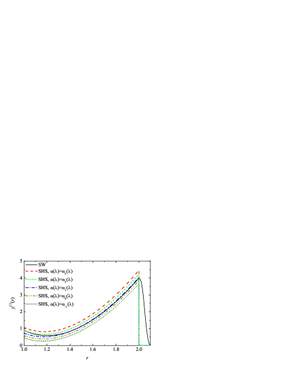
Figure 1: (Color online) Plot of the first-order virial coefficient of the cavity function, $y^{\text{(1)}}(r)$, for an SW fluid with $\lambda=1.05$ and $T^{*}=0.35$ and for SHS fluids with values of $\tau$ given by Eqs. (22) and (23) with $n=3$, $n=2$, $n=1$, $n\to 0$, and $n=-1$.

This is the same choice as considered by de Kruif et al.KRBDVM89 . With this definition, the difference between $y_{\text{SW}}^{(1)}$ and $y_{\text{SHS}}^{(1)}$ in the range $1<r<2$ becomes

$$y_{\text{SW}}^{(1)}(r|T^{*},\lambda)-y_{\text{SHS}}^{(1)}(r|\tau_{\text{eff}}(T^{*},\lambda))=\frac{1+6(2-4r+r^{2})\tau_{\text{eff}}}{12r\tau_{\text{eff}}^{2}}(\lambda-1)+\mathcal{O}((\lambda-1)^{2}).$$ (29)

Let us now explore the consequences of the approximation (14), complemented by Eqs.  (21) and (28), on some of the physical properties. We first note that a simple approximate expression can be obtained for the excess internal energy of the SW fluid in terms of the value of the SHS cavity function and its slope at $r=1$. First, we make the approximation $y_{\text{SW}}(r)\approx y_{\text{SHS}}(1)+y_{\text{SHS}}^{\prime}(1)(r-1)$ inside the integral of Eq. (II.1). Next we perform the integral, make use of Eq. (28) and neglect terms nonlinear in $\lambda-1$. The result is

$$-\frac{1}{\epsilon}u_{\text{SW}}\approx-\frac{1}{\epsilon}u_{\text{SHS}}\left[1+\left(1+12\tau_{\text{eff}}+\frac{y_{\text{SHS}}^{\prime}(1)}{2y_{\text{SHS}}(1)}\right)(\lambda-1)\right],$$ (30)

where the arguments denoting the dependence of the quantities on $\eta$, $T^{*}$ and $\lambda$ have been omitted for simplicity. Equation (30) shows that, even if the approximation (14) is satisfied, $u_{\text{SW}}(\eta,T^{*};\lambda)\neq u_{\text{SHS}}(\eta,\tau_{\text{eff}}(T^{*};\lambda))$.

Analogously, making $y_{\text{SW}}(r)\approx y_{\text{SHS}}(1)+y_{\text{SHS}}^{\prime}(1)(r-1)$ in the interval $1<r<\lambda$, Eq. (4) yields

$$S_{\text{SW}}(k)-S_{\text{SHS}}(k) \approx \frac{\eta}{k\tau_{\text{eff}}}\left[y_{\text{SHS}}(1)(k\cos k+\sin k)\right.$$ (31)

$$\left.+y_{\text{SHS}}^{\prime}(1)\sin k\right](\lambda-1),$$

where again terms nonlinear in $\lambda-1$ have been neglected and the arguments denoting the dependence of the quantities on $\eta$, $T^{*}$, and $\lambda$ have been omitted. Taking the limit $k\to 0$ in the above expression, we have

$$\chi_{\text{SW}}-\chi_{\text{SHS}}\approx\frac{\eta}{\tau_{\text{eff}}}\left[2y_{\text{SHS}}(1)+y_{\text{SHS}}^{\prime}(1)\right](\lambda-1).$$ (32)

Finally, from Eqs. (5) and (11) one gets

$$Z_{\text{SW}}-Z_{\text{SHS}}\approx-\frac{\eta}{\tau_{\text{eff}}}\left[y_{\text{SHS}}(1)+\frac{1}{6}y_{\text{SHS}}^{\prime\prime}(1)\right](\lambda-1)$$ (33)

Equations (30)–(33) must be interpreted as simple heuristic approximations relating some physical properties of SHS and short-range SW fluids. Thus, they do not give the first-order terms in a systematic expansion in powers of $\lambda-1$ because they are based on the ansatz (14), which ignores terms of order $\lambda-1$ in the difference $y_{\text{SW}}(r)-y_{\text{SHS}}(r)$, as shown by Eq. (29). Note also that Eqs. (30)–(33) depend on our choice (28) for $\tau_{\text{eff}}$.

IV Comparison with simulations of sticky hard spheres

We have performed conventional Monte Carlo simulations using the canonical ensemble and employing the linked cell-list method in a cubic box with a standard periodic boundary conditions. $N=4000$ particles interacting via the SW potential (1) were displaced according to the Metropolis algorithm to create a sample of configurations. The calculation of the desired quantities (internal energy and radial distribution function) was organized in cycles. Any randomly chosen particle was attempted to move and the cycle was repeated $100\times N$ times for equilibration before the system was analyzed. The process was repeated $1000$ times to get one averaged set of values. Each run was divided into 20 such blocks, so that at least $10^{9}$ configurations were generated. The distance of attempted displacements was a mixture of one value adjusted for each $\lambda$ so that the acceptance ratio was 10%–15% and another value ten times shorter to take care of tiny attractive effects.

$\eta$	$\tau_{\text{eff}}$	$\lambda$	$T^{*}$	$y(1)$	$y^{\prime}(1)$	$-u/\epsilon$	Eq. (30)
$0.164$	$0.13$	$1.05$	$0.381$	$0.904$	$-0.314$	$1.271$	$1.273$
		$1.02$	$0.286$	$0.907$	$-0.293$	$1.203$	$1.191$
		$1.01$	$0.239$	$0.908$	$-0.307$	$1.185$	$1.164$
		$1$	$0$	$0.901$	$-0.280$	$1.137$	$1.137$
$0.32$	$0.2$	$1.05$	$0.448$	$0.935$	$-0.757$	$1.724$	$1.709$
		$1.02$	$0.324$	$0.927$	$-0.685$	$1.573$	$1.573$
		$1.01$	$0.266$	$0.924$	$-0.708$	$1.520$	$1.528$
		$1$	$0$	$0.927$	$-0.661$	$1.483$	$1.483$
$0.4$	$0.5$	$1.05$	$0.682$	$1.622$	$-4.161$	$1.664$	$1.604$
		$1.02$	$0.448$	$1.580$	$-3.773$	$1.408$	$1.387$
		$1.01$	$0.348$	$1.563$	$-3.697$	$1.328$	$1.314$
		$1$	$0$	$1.552$	$-3.606$	$1.242$	$1.242$

Table 1: SW systems simulated and corresponding values of $y(1)$, $y^{\prime}(1)$, and $-u/\epsilon$.

Figure 2: (Color online) Cavity function at $\eta=0.164$ and $\tau_{\text{eff}}=0.13$. The solid line corresponds to MC simulations for SHS by Miller and Frenkel.MF04a The dotted, dashed, and dash-dotted curves correspond to our simulations for SW systems with $\lambda=1.05$, $1.02$, and $1.01$, respectively.

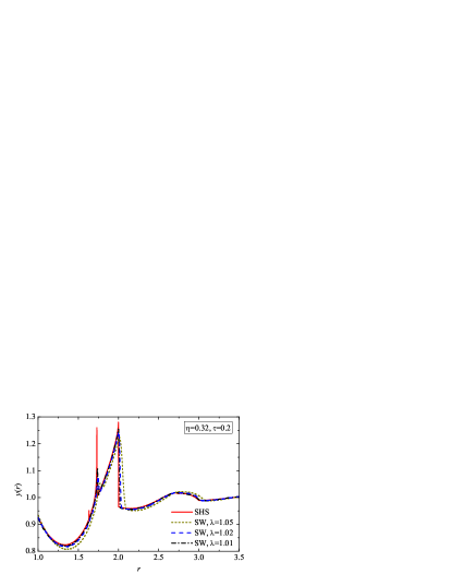
Figure 3: (Color online) Same as in Fig. 1 but for $\eta=0.32$ and $\tau_{\text{eff}}=0.2$.

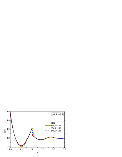
Figure 4: (Color online) Same as in Fig. 1 but for $\eta=0.4$ and $\tau_{\text{eff}}=0.5$.

We have considered three different ranges: $\lambda=1.05$, $1.02$. and $1.01$. In each case, a temperature $T^{*}$ has been chosen such that the effective stickiness parameter $\tau_{\text{eff}}$ defined by Eq. (28) takes the same value. In order to test the approximation (14), the values of $\eta$ and $\tau_{\text{eff}}$ have been taken the same as those considered by Miller and Frenkel in Ref. MF04a, . They are listed in Table 1, where also the internal energy $-u/\epsilon$ and the values at contact $y(1)$ and $y^{\prime}(1)$ are included. The two latter quantities have been obtained from a quadratic fit of the simulation data for $y_{\text{SW}}(r)$ and $y_{\text{SHS}}(r)$ in the interval $1<r<1.1$. Inasmuch as Eq. (14) is a reasonable approximation, one would expect that, at a given state point $(\eta,\tau_{\text{eff}})$, the four cavity functions, i.e., $y_{\text{SHS}}(r)$ and $y_{\text{SW}}(r)$ with $\lambda=1.05$, $1.02$, and $1.01$, overlap to some extent. Table 1 shows that the contact value of the cavity function, $y(1)$, and its first derivative, $y^{\prime}(1)$, are indeed quite similar for the four systems at each state. At the smallest temperature ($\tau_{\text{eff}}=0.13$), the values of $y(1)$ agree within statistical errors. At the intermediate temperature ($\tau_{\text{eff}}=0.2$), $y_{\text{SW}}(1)$ for $\lambda=1.05$ deviates from $y_{\text{SHS}}(1)$ less than 1%, while $y_{\text{SW}}(1)$ for $\lambda=1.02$ and for $\lambda=1.01$ practically coincide with $y_{\text{SHS}}(1)$. At the highest temperature ($\tau_{\text{eff}}=0.5$), $y_{\text{SW}}(1)$ differs from $y_{\text{SHS}}(1)$ less than 5%, 2%, and 1% for $\lambda=1.05$, 1.02, and 1.01, respectively. The fact that the agreement between $y_{\text{SW}}(1)$ and $y_{\text{SHS}}(1)$ slightly decreases as the temperature increases is associated with the choice of $\tau_{\text{eff}}$ given by Eq. (28). As discussed in Sec. III, that choice was expected to be better for temperatures such that $\tau_{\text{eff}}\sim 0.1$ than for larger ones. Similar conclusions can be drawn from the comparison of $y_{\text{SW}}^{\prime}(1)$ and $y_{\text{SHS}}^{\prime}(1)$, although in that case we have observed that the influence of the noise of the simulation data and that of the fitting procedure are slightly larger than in the case of $y(1)$.

Even if $y_{\text{SW}}(r)\approx y_{\text{SHS}}(r)$, that does not mean that $u_{\text{SW}}\approx u_{\text{SHS}}$ since the excess internal energy monitors the correlation function in the range $1<r<\lambda$ and so it is sensitive to the width of the well. In fact, Table 1 shows that the magnitude of the excess internal energy changes much more than the contact value of the cavity function when shrinking the well width. On the other hand, Eq. (30), which is implemented in Table 1 with the simulation data of $y_{\text{SHS}}(1)$ and $y_{\text{SHS}}^{\prime}(1)$, incorporates terms linear in $\lambda-1$ and so it provides a very good estimate of the SW internal energy.

A more complete comparison between $y_{\text{SW}}(r)$ and $y_{\text{SHS}}(r)$ is provided by Figs. 2–4. There it is shown that the global shape of $y_{\text{SW}}(r|\eta,T^{*};\lambda)$ at fixed $\eta$ and $\tau_{\text{eff}}(T^{*},\lambda)$ is only weakly influenced by the value of $\lambda$. In particular, the precursors of the singularities (delta-peaks and/or discontinuities)SG87 ; MF04a of $y_{\text{SHS}}(r)$ at $r=\sqrt{\frac{8}{3}},\frac{5}{3},\sqrt{3},2,\ldots$ are clearly apparent in the SW fluids, especially for $\lambda=1.01$. Apart from those local singularities, one can observe that the SW cavity function for $\lambda\leq 1.02$ is reasonably well described by the SHS one, while slight but visible deviations are present in the case $\lambda=1.05$.

It must be emphasized again that the good agreement between the SHS and SW cavity functions does not imply the same in the case of the radial distribution function inside the well ($1\leq r\leq\lambda$). As a consequence, the structure factor, being related to the Fourier transform of $h(r)$, can be expected to be affected by the difference between $g_{\text{SHS}}(r)$ and $g_{\text{SW}}(r)$ near $r=1$. To visualize this effect, we compare in Figs. 5–7 the SHS and SW structure factors, in the latter case with $\lambda=1.02$. Although both functions are very close each other in the three cases, some systematic differences are apparent. In particular, the maxima and minima of $S_{\text{SW}}(k)$ are slightly more pronounced and shifted to the left than those of $S_{\text{SHS}}(k)$. The difference $\Delta S(k)\equiv S_{\text{SW}}(k)-S_{\text{SHS}}(k)$ is plotted in the insets of Figs. 5–7. Except for small $k$, it is observed that the simulation data of $\Delta S(k)$ are remarkably well described by the approximation (31), where the simulation values for $y_{\text{SHS}}(1)$ and $y_{\text{SHS}}^{\prime}(1)$ are used. This confirms that the differences between $y_{\text{SW}}(r)$ and $y_{\text{SHS}}(r)$, which are neglected in Eq. (31), have a practically irrelevant influence on the difference between $S_{\text{SW}}(k)$ and $S_{\text{SHS}}(k)$.

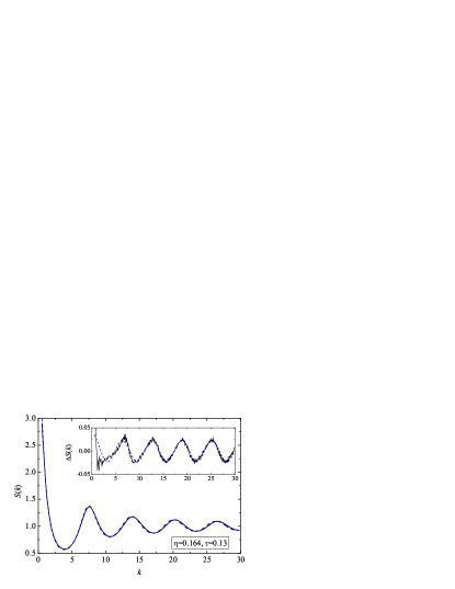
Figure 5: (Color online) Structure factor $S(k)$ at $\eta=0.164$ and $\tau_{\text{eff}}=0.13$. The solid line corresponds to MC simulations for SHS by Miller and Frenkel.MF04a The dashed curve corresponds to our simulations for an SW system with $\lambda=1.02$. The inset shows the difference $\Delta S(k)\equiv S_{\text{SW}}(k)-S_{\text{SHS}}(k)$ as obtained from simulations (solid line) and as given by Eq. (31) (dashed line).

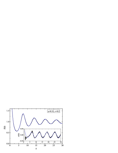
Figure 6: (Color online) Same as in Fig. 5 but for $\eta=0.32$ and $\tau_{\text{eff}}=0.2$.

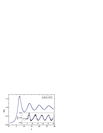
Figure 7: (Color online) Same as in Fig. 5 but for $\eta=0.4$ and $\tau_{\text{eff}}=0.5$.

V Comparison with theoretical predictions

The approximate mapping $y_{\text{SW}}(r)\to y_{\text{SHS}}(r)$ can be exploited to get theoretical predictions for the radial distribution function $g_{\text{SW}}(r)$ of short-range SW fluids from the availability of analytical expressions for $g_{\text{SHS}}(r)$. In particular, we will use Baxter’s solution of the PY equation for SHS,B68 as well as an extension of it proposed by two of us.YS93b For the sake of completeness, we will also consider an alternative theoretical approach directly devised for SW fluids.YS94 ; AS01 ; LSAS03 Before comparing with our MC simulations, the expressions stemming from these three theories are briefly described.

V.1 Percus–Yevick and rational-function approximations for sticky hard spheres

As is well known, Baxter was able to find the exact solution of the PY theory for the case of SHS.B68 This solution was later interpreted as the simplest case of a more general class of approximations.YS93a ; YS93b Both approaches are constructed in the Laplace space. Let us introduce the Laplace transform of $rg(r)$:

$$G(s)\equiv\int_{1}^{\infty}{d}r\,e^{-rs}rg(r)=s\frac{F(s){e}^{-s}}{1+12\eta F(s){e}^{-s}},$$ (34)

where the last equality defines the auxiliary function $F(s)$. In real space,

$$g(r)=\frac{1}{r}\sum_{n=1}^{\infty}(-12\eta)^{n-1}f_{n}(r-n)\Theta(r-n),$$ (35)

where $f_{n}(r)$ is the inverse Laplace transform of $s[F(s)]^{n}$ and $\Theta(x)$ is Heaviside’s step function. The auxiliary function $F(s)$ must comply with some consistency conditions for small $s$ and for large $s$:YS93a ; YS93b

$$\frac{{e}^{s}}{F(s)}=-12\eta+s^{3}+\mathcal{O}(s^{5}),$$ (36)

$$F(s)=y(1)s^{-1}\left(\frac{1}{12\tau}+s^{-1}\right)+\mathcal{O}(s^{-3}).$$ (37)

A simple class of approximations consists of assuming a rational form for $F(s)$:

$$F(s)=-\frac{1}{12\eta}\frac{1+\sum_{j=1}^{m}L_{j}s^{j}}{1+\sum_{j=1}^{m+1}S_{j}s^{j}},$$ (38)

with $m\geq 2$. The simplest case corresponds to $m=2$, the coefficients $L_{1}$, $L_{2}$, $S_{1}$, $S_{2}$, and $S_{3}$ being explicitly determined YS93a from the application of the physical constraints (36) and (37). This leads to the exact solution of the PY equation for SHS. B68 One of the shortcomings of this PY-SHS theory is that it yields inconsistent equations of state via the energy and compressibility routes.

A more flexible approximation is obtained by setting $m=3$ in Eq. (38) and fixing the additional parameters $L_{3}$ and $S_{4}$ by consistently imposing a given equation of state through the contact value $y(1)$ and the isothermal susceptibility $\chi$.YS93b We will refer to the ansatz (38) with $L_{3}$ and $S_{4}$ determined in this way as the rational-function approximation for SHS (RFA-SHS). Given a compressibility factor $Z_{\text{SHS}}(\eta,\tau)$ for the SHS fluid, the isothermal compressibility and the excess internal energy are obtained asYS93a

$$\chi_{\text{SHS}}^{-1}=\frac{\partial}{\partial\eta}\left(\eta Z_{\text{SHS}}\right),$$ (39)

$$\frac{u_{\text{SHS}}}{\epsilon}=-\tau\frac{\partial}{\partial\tau}\int_{0}^{\eta}{d}\eta^{\prime}\frac{Z_{\text{SHS}}(\eta^{\prime},\tau)-1}{\eta^{\prime}}.$$ (40)

The contact value $y_{\text{SHS}}(1)$ consistent with $Z_{\text{SHS}}$ can then be obtained from the internal energy through Eq. (13). For the compressibility factor $Z_{\text{SHS}}(\eta,\tau)$ we will use the empirical form recently proposed by Miller and Frenkel.MF04b

V.2 Rational-function approximations for square-well fluids

In the case of SW fluids with a hard-core diameter $\sigma=1$ and range $\lambda$ one can still define the auxiliary function $F(s)$ trough Eq. (34), so that Eqs. (35) and (36) also hold in this case.YS93a ; YS93b However, the constraint (37) is now replaced by

$$F(s)=g(1^{+})s^{-2}+\mathcal{O}(s^{-3}).$$ (41)

In the spirit of the ansatz (38), the simplest rational-function approximation for SW systems (RFA-SW) has the formYS94 ; AS01

$$F(s)=-\frac{1}{12\eta}\frac{1+A+K_{1}s-(A+K_{2}s){e}^{-(\lambda-1)s}}{1+S_{1}s+S_{2}s^{2}+S_{3}s^{3}}.$$ (42)

Application of the condition (36) allows one to express $K_{1}$, $S_{1}$, $S_{2}$, and $S_{3}$ as linear functions of $A$ and $K_{2}$. Next, $A$ is taken for simplicity as independent of density, so that $A={e}^{1/T^{*}}-1$. Finally, $K_{2}$ is obtained by enforcing the continuity of $y(r)$ at $r=\lambda$.

It can be provedYS94 that in the SHS limit ($\lambda\to 1$, $T^{*}\to 0$ with $\tau=\text{finite}$), one has $K_{2}(\lambda-1)\to L_{2}$ and $K_{1}-K_{2}+A(\lambda-1)\to L_{1}$, so that Eq. (42) reduces to Eq. (38) with $m=2$, i.e., the PY-SHS solution. An improved RFA-SW theory that would reduce to the RFA-SHS theory would require the addition of new terms in the numerator and denominator of Eq. (42), but then extra constraints would be needed to determine those new coefficients.

V.3 Comparison

We are now in conditions of comparing the three theories against our MC simulation data. We restrict ourselves to the case $\lambda=1.05$. Since the radial distribution function $g(r)$ is a more direct and intuitive quantity than the cavity function $y(r)$, we present the plots in terms of $g(r)$ in Figs. 8–10.

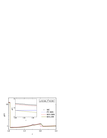
Figure 8: (Color online) Radial distribution function of an SW fluid with $\lambda=1.05$ at $\eta=0.164$ and $T^{*}=0.381$. The circles correspond to our MC simulations and the solid lines represent the RFA-SW predictions. The results obtained from the approximation (14) with $\tau_{\text{eff}}=0.13$ by using the PY and RFA theories for the SHS fluid are represented by the dotted and dashed lines, respectively. The inset shows $g(r)$ inside the well. Outside that region, the PY-SHS and RFA-SHS curves are practically indistinguishable.

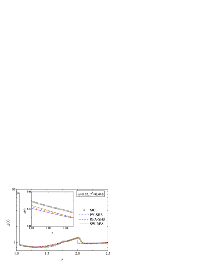
Figure 9: (Color online) Same as in Fig. 9 but for $\eta=0.32$, $T^{*}=0.448$ and $\tau_{\text{eff}}=0.2$.

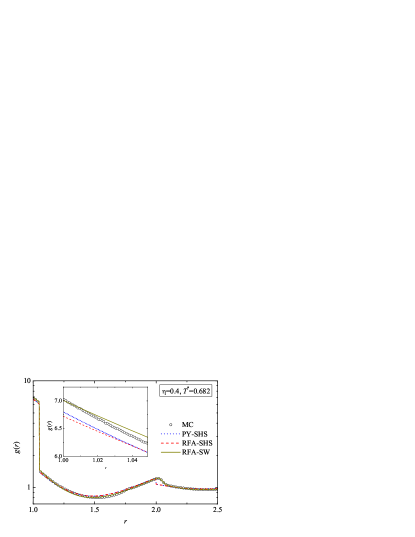
Figure 10: (Color online) Same as in Fig. 9 but for $\eta=0.4$, $T^{*}=0.682$ and $\tau_{\text{eff}}=0.5$.

We observe a good general agreement between theories and simulations for the three states. This is noteworthy since no fitting has been employed. Only in the case of the RFA-SHS approach there exist two free parameters ($L_{3}$ and $S_{4}$) which are determined by enforcing thermodynamic consistency with an empirical equation of state for SHS fluids,MF04b as explained above. Despite the good theoretical behaviour, none of the theories predict the distortion around $r=1.77$, which is the precursor of the singularity of the exact $g_{\text{SHS}}$ at $r=\sqrt{3}\approx 1.73$. Obviously, the PY-SHS and RFA-SHS approximations transfer to $g_{\text{SW}}$ the discontinuity of $g_{\text{SHS}}$ at $r=2$, while the RFA-SW approximation accurately captures the rapid but continuous decay of $g_{\text{SHS}}$ near $r=2$. In general, both SHS theories yield results which are practically indistinguishable, especially for the two highest temperatures ($T^{*}=0.448$ and $T^{*}=0.682$). Only inside the attractive well ($1\leq r\leq 1.05$) can one distinguish the PY-SHS and RFA-SHS predictions, as shown in the insets. This region is especially important for SW fluids since it is directly related to the coordination number and the excess internal energy. We observe that the best performance in the region $1\leq r\leq 1.05$ is done by the RFA-SHS theory at the lowest temperature ($T^{*}=0.381$) and by the RFA-SW theory at the other two temperatures ($T^{*}=0.448$ and $T^{*}=0.682$). In this respect, it must be borne in mind that the choice (28) of the effective stickiness parameter is more appropriate for temperatures such that $\tau_{\text{eff}}\approx 0.1$ than for higher temperatures.

VI Mixtures of SW fluids

Let us now consider the case of multicomponent systems of particles interacting via SW potentials:

$$\varphi_{ij}^{\text{SW}}(r)=\begin{cases}\infty,&r<\sigma_{ij},\\ -\epsilon_{ij},&\sigma_{ij}<r<\lambda_{ij}\sigma_{ij},\\ 0,&r>\lambda_{ij}\sigma_{ij}.\end{cases}$$ (43)

In the one-component case, there are three parameters characterizing the interaction ($\sigma$, $\epsilon$, and $\lambda$) and two parameters defining the thermodynamic state ($\rho$ and $T$). Without loss of generality, we can use $\sigma$ and $\epsilon$ to fix the units of distance and energy, respectively, so that only three independent dimensionless parameters remain ($\lambda$, $\eta$, and $T^{*}$). In the case of mixtures, however, the number of parameters is in general much higher. Restricting ourselves to the binary case, we have three thermodynamic quantities (the total density $\rho$, the mole fraction $x_{1}$ of one of the species, and the temperature $T$) plus nine interaction parameters (the diameters $\sigma_{ij}$, the well depths $\epsilon_{ij}$, and the relative ranges $\lambda_{ij}$). One of the diameters can be used to define the length unit and one of the depths can be used to define the energy unit, so that the number of independent parameters defining the problem is ten in general.note1

The SW potentials (43) become SHS potentials if $\lambda_{ij}\to 1$ and $\epsilon_{ij}\to\infty$ by keeping constant the parameters

$$\tau_{ij}^{\text{eff}}=\frac{1}{12({e}^{\epsilon_{ij}/k_{B}T}-1)(\lambda_{ij}-1)}.$$ (44)

Now, each pair $(\epsilon_{ij},\lambda_{ij})$ gives birth to a parameter $\tau_{ij}^{\text{eff}}$ and so the general number of parameters characterizing the binary mixture reduces from ten to seven. Note that, although the term $-1$ appearing in the denominator of Eq. (44) can be neglected in the SHS limit, we have kept it so that Eq. (44) defines the generalization to mixtures of the effective stickiness parameter defined by Eq. (28). The exact solution of the PY equation for SHS mixtures is knownPS75 in the additive case $\sigma_{ij}=(\sigma_{ii}+\sigma_{jj})/2$. Systems of SHS mixtures have been considered by several authors.BT79 ; JBH91 ; TKR02 ; GG02 ; FGG05 ; J06 An extension of the RFA described in Subsec. V.1 to SHS mixtures is also available.SYH98

In agreement with the philosophy behind the approximation (14) for the one-component case, we can expect that, for narrow SW potentials,

$$y_{ij}^{\text{SW}}(r|\rho,x_{1},T,\{\sigma_{k\ell}\},\{\epsilon_{k\ell}\},\{\lambda_{k\ell}\})\approx y_{ij}^{\text{SHS}}(r|\rho,x_{1},\{\sigma_{k\ell}\},\{\tau_{k\ell}^{\text{eff}}\}),$$ (45)

where $y_{ij}(r)\equiv{e}^{\varphi_{ij}(r)/k_{B}T}g_{ij}(r)$.

Given the high dimensionality of the parameter space for binary SW mixtures, we restrict ourselves to the two classes of mixtures shown in Table 2. Class I corresponds to equimolar and symmetric mixtures in which the self interactions 1-1 and 2-2 are of HS type, while the cross interaction 1-2 is of SW type. Therefore, $\tau_{11}^{\text{eff}}=\tau_{22}^{\text{eff}}=\infty$ and $\tau_{12}^{\text{eff}}=\tau_{\text{eff}}$. This class of mixtures can be used to describe adsorption phenomena.BT79 Class II is representative of asymmetric hard-core diameters, but with common well depths and relative well widths, so that $\tau_{ij}^{\text{eff}}=\tau_{\text{eff}}$. It only remains to fix for each class the values of the range $\lambda$, the reduced temperature $T^{*}=k_{B}T/\epsilon$ and the reduced density $\rho\sigma^{3}$ or, equivalently, the total packing fraction $\eta=\pi\rho(x_{1}\sigma_{11}^{3}+x_{2}\sigma_{22}^{3})/6$. The values considered in this paper for those quantities are shown in Table 3. This yields a total of 12 different mixtures simulated. For each $\lambda$, the temperature is chosen so that $\tau_{\text{eff}}=0.2$ and 0.5, in analogy with some of the cases considered in Table 1.

Class	$\sigma_{11}$	$\sigma_{22}$	$\sigma_{12}$	$\lambda_{11}$	$\lambda_{22}$	$\lambda_{12}$	$\epsilon_{11}$	$\epsilon_{22}$	$\epsilon_{12}$	$x_{1}$
I	1	1	1	1	1	$\lambda$	0	0	$\epsilon$	$\frac{1}{2}$
II	1	3	2	$\lambda$	$\lambda$	$\lambda$	$\epsilon$	$\epsilon$	$\epsilon$	$\frac{15}{16}$

Table 2: Classes of SW mixtures considered in the simulations.

$\eta$	$\tau_{\text{eff}}$	$\lambda$	$T^{*}$
0.4	0.2	1.05	0.448
		1.02	0.324
		1.01	0.266
	0.5	1.05	0.682
		1.02	0.448
		1.01	0.348

Table 3: Values of $\eta$, $\lambda$ and $T^{*}$ considered in the simulations.

Now we compare, for each class and each value of $\tau_{\text{eff}}$, the cavity functions $y_{ij}(r)$ obtained from our MC simulations. Given the scarcity of simulations for SHS mixtures,note2 we use the analytical solution of the PY closure.PS75 We cannot use the expressions provided by the RFA methodSYH98 because the latter relies upon the knowledge of the equation of state for SHS mixtures. While an accurate empirical equation of state exists for one-component SHS fluids,MF04b its extension to mixtures is not known.

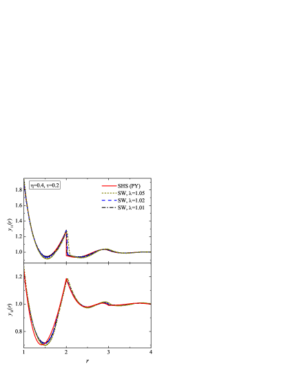
Figure 11: (Color online) Cavity functions at $\eta=0.4$ and $\tau_{\text{eff}}=0.2$ for a binary mixture of class I (see Table 2). The solid lines correspond to the analytical solution of the PY theory for SHS mixtures. The dotted, dashed, and dash-dotted curves correspond to our simulations for SW systems with $\lambda=1.05$, $1.02$, and $1.01$, respectively.

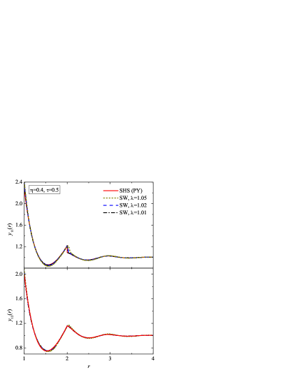
Figure 12: (Color online) Same as in Fig. 11 but for $\eta=0.4$ and $\tau_{\text{eff}}=0.5$.

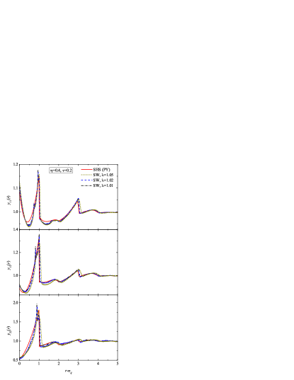
Figure 13: (Color online) Cavity functions at $\eta=0.4$ and $\tau_{\text{eff}}=0.2$ for a binary mixture of class II (see Table 2). The solid lines correspond to the analytical solution of the PY theory for SHS mixtures. The dotted, dashed, and dash-dotted curves correspond to our simulations for SW systems with $\lambda=1.05$, $1.02$, and $1.01$, respectively.

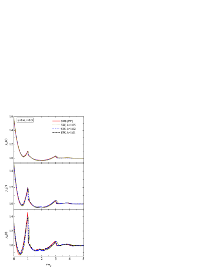
Figure 14: (Color online) Same as in Fig. 13 but for $\eta=0.4$ and $\tau_{\text{eff}}=0.5$.

The two states corresponding to mixtures of class I are considered in Figs. 11 and 12. We observe that the range $\lambda=1.05$ is again not small enough to produce a good overlap with the cases $\lambda=1.02$ and $\lambda=1.01$. These two latter SW mixtures can be expected to be close to the true SHS mixture. In this respect, the deviations of our SW simulations with $\lambda=1.02$ and $\lambda=1.01$ from the SHS-PY theory reveal the limitations of the latter.J06 Figures 11 and 12 show that the PY theory describes better the pair correlation function $y_{11}=y_{22}$ of the particles interacting via the HS potential than the pair correlation function $y_{12}$ of the particles feeling a short-range attraction. Accordingly, the agreement improves when the temperature increases (from $\tau_{\text{eff}}=0.2$ to $\tau_{\text{eff}}=0.5$) and hence the stickiness decreases.

The results corresponding to the asymmetric mixtures of class II are plotted in Figs. 13 and 14. The convergence SW$\to$SHS is similar to that in the symmetric cases since the deviations between the curves corresponding to the ranges $\lambda=1.02$ and $\lambda=1.01$ are again small. However, the performance of the PY theory is worse in Figs. 13 and 14 than in Figs. 11 and 12. This could have been expected by the following arguments. On the one hand, the presence of stickiness is larger in class II than in class I. On the other hand, it is known that the PY theory is more accurate for one-component HS fluids (class I in the limit $\tau\to\infty$) than for HS mixtures (class II in the limit $\tau\to\infty$).MMYSH02

VII Summary and concluding remarks

In this paper we have investigated the possibility of representing the structural and thermodynamic properties of short-range SW fluids by those of SHS fluids. It is sometimes assumed in the literature on colloidal suspensions that a range $\lambda\leq 1.1$ is small enough to replace the more realistic SW model by the simpler SHS model. Moreover, the mapping SW$\to$SHS is usually assumed to hold at the level of the structure factor, i.e., $S_{\text{SW}}(k)\approx S_{\text{SHS}}(k)$. This in turn implies $g_{\text{SW}}(r)\approx g_{\text{SHS}}(r)$, what misses the fact that $g_{\text{SW}}(r)$ has a jump discontinuity at $r=\lambda$ which becomes a delta singularity of $g_{\text{SHS}}(r)$ at $r=1^{+}$.

Here, however, the ansatz $S_{\text{SW}}(k)\approx S_{\text{SHS}}(k)$ or, equivalently, $g_{\text{SW}}(r)\approx g_{\text{SHS}}(r)$ has been replaced by $y_{\text{SW}}(r)\approx y_{\text{SHS}}(r)$. This still leaves open the problem of finding the effective packing fraction $\eta_{\text{eff}}$ and the effective stickiness parameter $\tau_{\text{eff}}$ of the SHS fluid that best mimics the physical properties of an SW fluid of range $\lambda$ at a given state $(\eta,T^{*})$. For simplicity, we have chosen $\eta_{\text{eff}}$ to be independent of $T^{*}$ and $\tau_{\text{eff}}$ to be independent of $\eta$. Next, the constraint of recovering the HS fluid in the limit $T^{*}\to\infty$ leads to $\eta_{\text{eff}}=\eta$ in a natural way. Since $\tau_{\text{eff}}$ is assumed to be independent of $\eta$, we have taken advantage of the exact knowledge of $y_{\text{SW}}(r)$ and $y_{\text{SHS}}(r)$ to first order in density as a guide to choose $\tau_{\text{eff}}$. Considering several possibilities of the form (22), we have found that the optimal choice for temperatures such that $\tau_{\text{eff}}\approx 0.1$ is provided by Eq. (28), as illustrated by Fig. 1. This choice differs from the conventional one,SG87 ; RR89 ; TB93 ; VL00 based on the equality of the SW and SHS second virial coefficients, i.e., $B_{2}^{\text{SW}}(T^{*};\lambda)=B_{2}^{\text{SHS}}(\tau_{\text{eff}}(T^{*},\lambda))$.

The condition $B_{2}^{\text{SW}}=B_{2}^{\text{SHS}}$ is directly related to the assumption that the thermodynamic properties of the SW and SHS fluids are the same, at least for low densities. Our approach differs from this one. We have assumed that the cavity function is approximately the same in both systems and from this ansatz we have obtained expressions for the structure factor, the internal energy, the isothermal compressibility, and the pressure of the SW fluid in terms of quantities related to the SHS fluid. Those approximate relations have been checked by simulation data in the case of the structure factor (see Figs. 5–7) and the internal energy (see Table 1).

We have performed MC simulations of one-component SW fluids for $\lambda=1.05$, 1.02, and 1.01. For each case, we have considered the densities and temperatures indicated in Table 1. They correspond to the same values of the packing fraction and effective stickiness as considered by Miller and Frenkel in their simulations of SHS fluids.MF04a The comparisons (see Figs. 2–4) show that the SW cavity functions with $\lambda=1.05$ present small but visible differences with respect to the SHS ones. On the other hand, the SW curves corresponding to $\lambda=1.02$ and 1.01 have almost collapsed to the SHS curves, exhibiting the precursors of the singularities of $y_{\text{SHS}}(r)$ at $r=\sqrt{\frac{8}{3}},\frac{5}{3},\sqrt{3},2,\ldots$

While the PY equation has an exact solution for SHS, its solution for SW is not known exactly. However, we have exploited the knowledge of the PY-SHS solution,B68 as well as of the rational-function approximation (RFA) for SHS,YS93b to estimate the radial distribution function $g_{\text{SW}}(r)$ based on the ansatz $y_{\text{SHS}}(r)\approx y_{\text{SW}}(r)$. The results for $\lambda=1.05$ show a good general agreement with the MC data (see Figs. 8–10), except near $r=2$, where $g_{\text{SW}}(r)$ decays rapidly but does not present the jump discontinuity of $g_{\text{SHS}}(r)$. From that point of view, a better agreement is provided by the RFA-SW theory.YS94

In order to offer a wider perspective, we have also considered two classes of binary mixtures (see Table 2). Class I defines a symmetric equimolar mixture where the interactions among particles of the same species are of HS type, while those among particles of different species are of SW type. Mixtures of class II are asymmetric with a hard-core ratio 1:3 but with an attractive interaction of common depth and (relative) width. Comparison between our simulation data for SW mixtures and the theoretical PY-SHS predictionsPS75 shows that the latter behaves better for mixtures of class I (see Figs. 11 and 12) than for mixtures of class II (see Figs. 13 and 14). In each case, the agreement improves as the temperature increases (and hence the stickiness decreases). Apart from this comparison with the PY-SHS theory, our MC simulations show again that the range $\lambda=1.05$ is not small enough to get a good collapse with the cases $\lambda=1.02$ and 1.01.

One of the open avenues not fully explored in this paper refers to the analysis of the equation of state for short-range SW fluids obtained from the empirical equation of state for SHS fluids recently proposed by Miller and Frenkel.MF04b Equations (30), (32), and (33) provide three (approximate) alternative routes to the SW equation of state. They require the knowledge of $y_{\text{SHS}}(1)$, $y^{\prime}_{\text{SHS}}(1)$, and $y^{\prime\prime}_{\text{SHS}}(1)$. The two former quantities can be obtained from the SHS equation of state through Eqs. (11) and (13), while $y^{\prime\prime}_{\text{SHS}}(1)$ can be obtained from the RFA-SHS theory.YS93b We plan to undertake this study in the near future.

Appendix A The cavity function to first order in density

To first order in density, the cavity function of the SW fluid is given by Eq. (24). The coefficient $y_{\text{SW}}^{(1)}$ isBH67

$$y_{\text{SW}}^{(1)}(r|T^{*};\lambda)=A(r)+({e}^{1/T^{*}}-1)B_{\text{SW}}(r|\lambda)+({e}^{1/T^{*}}-1)^{2}C_{\text{SW}}(r|\lambda),$$ (46)

where (for $\lambda\leq 3$)

$$A(r)=\begin{cases}8-6r+\frac{1}{2}r^{3},&r<2,\\ 0,&r>2,\end{cases}$$ (47)

$$B_{\text{SW}}(r|\lambda)=\begin{cases}-12r+r^{3},&r<\lambda-1,\\ 3(\lambda^{2}-1)^{2}r^{-1}-8(\lambda^{3}-1)+6(\lambda^{2}-1)r,&\lambda-1<r<2,\\ 3(\lambda^{2}-1)^{2}r^{-1}-8(\lambda^{3}+1)+6(\lambda^{2}+1)r-r^{3},&2<r<\lambda+1,\\ 0,&r>\lambda+1,\end{cases}$$ (48)

$$C_{\text{SW}}(r|\lambda)=\begin{cases}8(\lambda^{3}-1)-6(\lambda^{2}+1)r+r^{3},&r<\lambda-1,\\ 3(\lambda^{2}-1)^{2}r^{-1},&\lambda-1<r<2,\\ 3(\lambda^{2}-1)^{2}r^{-1}-8+6r-\frac{1}{2}r^{3},&2<r<\lambda+1,\\ 8\lambda^{3}-6\lambda^{2}r+\frac{1}{2}r^{3},&\lambda+1<r<2\lambda,\\ 0,&r>2\lambda.\end{cases}$$ (49)

Taking the SHS limit, Eq. (46) reduces to

$$y_{\text{SHS}}^{(1)}(r|\tau)=A(r)+\frac{1}{12\tau}B_{\text{SHS}}(r)+\frac{1}{(12\tau)^{2}}C_{\text{SHS}}(r),$$ (50)

where

$$B_{\text{SHS}}(r)=\begin{cases}12(r-2),&0<r<2,\\ 0,&r>2,\end{cases}$$ (51)

$$C_{\text{SHS}}(r)=\begin{cases}12r^{-1},&0<r<2,\\ 0,&r>2.\end{cases}$$ (52)

References

- (1) J. S. Huang, S. A. Safran, M. W. Kim, and G. S. Grest, Phys. Rev. Lett. 53, 592 (1984).
- (2) C. G. de Kruif, P. W. Rouw, W. J. Briels, M. H. G. Duits, A. Vrij, and R. P. May, Langmuir 5, 422 (1989).
- (3) J. A. Barker and D. Henderson, Rev. Mod. Phys. 48, 587 (1976).
- (4) R. J. Baxter, J. Chem. Phys. 49, 2770 (1968).
- (5) G. Stell, J. Stat. Phys. 63, 1203 (1991).
- (6) J. W. Perram and E. R. Smith, Chem. Phys. Lett. 35, 138 (1975).
- (7) B. Barboy and R. Tenne, Chem. Phys. 38, 369 (1979).
- (8) A. J. Post and E. D. Glandt, J. Chem. Phys. 84, 4585 (1986); N. A. Seaton and E. D. Glandt, ibid. 84, 4595 (1986); 86, 4668 (1986); 87, 1785 (1987).
- (9) W. G. T. Kranendonk and D. Frenkel, Mol. Phys. 64, 403 (1988).
- (10) C. Regnaut and J. C. Ravey J. Chem. Phys. 91, 1211 (1989).
- (11) A. Jamnik, D. Bratko and D. J. Henderson, J. Chem. Phys. 94, 8210 (1991); A. Jamnik, ibid. 105, 1051 (1996).
- (12) S. V. G. Menon, C. Manohar, and K. S. Rao, J. Chem. Phys. 95, 9186 (1991).
- (13) C. F. Tejero and M. Baus, Phys. Rev. E, 48, 3793 (1993).
- (14) S. B. Yuste and A. Santos, J. Stat. Phys. 72, 703 (1993).
- (15) S. B. Yuste and A. Santos, Phys. Rev. E 48, 4599 (1993).
- (16) C. Regnaut, S. Amokrane, and Y. Heno, J. Chem. Phys. 102, 6230 (1995); S. Amokrane and C. Regnaut, ibid. 106, 376 (1997); S. Amokrane, P. Bobola, and C. Regnaut Progr. Colloid Polym. Sci. 100, 186 (1996).
- (17) C. Tutschka, G. Kahl, and E. Riegler, Mol. Phys. 100, 1025 (2002).
- (18) D. Gazzillo and A. Giacometti, Mol. Phys. 100, 3307 (2002).
- (19) M. A. Miller and D. Frenkel. Phys. Rev. Lett., 90, 135702 (2003).
- (20) D. Gazzillo and A. Giacometti, J. Chem. Phys. 120, 4742 (2004).
- (21) M. A. Miller and D. Frenkel, J. Phys.: Condens. Matter, 16, S4901 (2004).
- (22) M. A. Miller and D. Frenkel, J. Chem. Phys., 121, 535 (2004).
- (23) R. Fantoni, D. Gazzillo, and A. Giacometti, Phys. Rev. E 72, 011503 (2005).
- (24) A. Jamnik, Chem. Phys. Lett. 423, 23 (2006).
- (25) J.-P. Hansen and I. R. McDonald, Theory of Simple Liquids (Academic Press, London, 1986).
- (26) S. B. Yuste and A. Santos, J. Chem. Phys. 101, 2355 (1994)
- (27) L. Acedo and A. Santos, J. Chem. Phys. 115, 2805 (2001).
- (28) G. A. Vliegenthart and H. N. W. Lekkerkerker, J. Chem. Phys. 112, 5364 (2000); M. G. Noro and D. Frenkel, ibid. 113, 2941 (2000).
- (29) J. A. Barker and D. Henderson, Can. J. Phys. 44, 3959 (1967).
- (30) J. Largo, J. R. Solana, L. Acedo, and A. Santos, Mol. Phys. 101, 2981 (2003); J. Largo, J. R. Solana, S. B. Yuste, and A. Santos, J. Chem. Phys. 122, 084510 (2005).
- (31) This number reduces to eight if we assume the Lorentz-Berthelot rule, according to which and .
- (32) A. Santos, S. B. Yuste, and M. López de Haro, J. Chem. Phys. 109, 6814 (1998).
- (33) We are not aware of simulations of SHS mixtures apart from the ones recently reported by Jamnik in Ref. J06, , which have been published after our SW simulations were finished.
- (34) Al. Malijevský, A. Malijevský, S. B. Yuste, A. Santos, and M. López de Haro, Phys. Rev. E 66, 061203 (2002).