Networks of strong ties

Abstract

Social networks transmitting covert or sensitive information cannot use all ties for this purpose. Rather, they can only use a subset of ties that are strong enough to be “trusted”. In this paper we consider transitivity as evidence of strong ties, requiring that each tie can only be used if the individuals on either end also share at least one other contact in common. We examine the effect of removing all non-transitive ties in two real social network data sets. We observe that although some individuals become disconnected, a giant connected component remains, with an average shortest path only slightly longer than that of the original network. We also evaluate the cost of forming transitive ties by deriving the conditions for the emergence and the size of the giant component in a random graph composed entirely of closed triads and the equivalent Erdös-Renyi random graph.

I INTRODUCTION

The strength of weak ties is the concept that individuals tend to be more successful in acquiring information about job opportunities by contacting individuals that they did not see often—their weak ties granovetter73ties . The rationale behind this idea is that close friends tend to have similar information to us because they share similar interests, profession, or geographical location. Weak ties on the other hand are between individuals who don’t have much in common, including other contacts, and the information they have access to will tend be different. A shared contact between two individuals forms a closed triad (triangle), where all three people know one another. Strong ties are usually parts of triads because good friends or close professional contacts of one person will tend to know one another. In this paper we make the simplifying assumption that ‘weak ties’ are those that are not part of any closed triad and we define ‘strong ties’ are the ones that share at least one other contact in common. In other contexts the strength of the tie may include measures such as frequency or length of contact, but for simplicity here we consider only the presence of closed triads.

While weak ties may be preferred in acquiring job information, one may be interested in assembling a team or otherwise gathering information that is distributed in different parts of a social network using only strong ties. In the case of the Madrid terrorist bombings on March 11th, 2003, the individuals behind the attack were able to procure knowledge about making explosive devices, hashish to trade for explosive materials, and the explosive material itself using their strong ties. Had they used weak ties which would have been less reliable, their plot may have been exposed and their intentions thwarted. Sinister plots are not the only example of a planning activity that can benefit from using strong ties to maintain confidentiality. Scientists may wish to forge collaborations requiring diverse expertise guimera2005team , and in doing so they may wish to keep a competitive edge by not broadcasting their ideas over weak ties. Similar situations may arise in the formation of business alliances, where companies seek to complement their strengths through mergers, acquisitions, cross licensing of intellectual property, or joint ventures, but do not wish to leak their next steps to competitors.

There are also processes which describe the contagion of new ideas and practices in which the credibility of information or the willingness to adopt an innovation requires independent confirmation from multiple sources. Unlike a ‘simple’ biological contagious agent carrying a disease, which can be transferred through a single contact between two individuals, ideas and opinions (‘complex’ agents) may need to be heard from multiple contacts before being adopted centola05 . Whether one considers teenagers deciding to buy a new brand of jeans or farmers starting to plant a new type of corn, the decisive event may not be hearing about an innovation, but observing enough people participating to be convinced that the innovation should be adopted strang98diffusion ; ryan43corn .

The presence of closed triads enhances the probability that complex contagion can spread on a network. Social networks tend to have a much higher probability of closed triads than the equivalent random networks Watts98smallworld ; newman03structure . An intuitive reason is given by structural balance theory Cartwright56balance which states that ties tend to be transitive: if a node is connected to two other nodes (is a member of two diads), those two nodes are much more likely on average to be connected than two randomly chosen nodes. Recently, it has also been shown that many real world networks, including social networks, contain overlapping k-cliques Palla05community . Within a k-clique, each of the $k$ nodes is connected to each of the other $k$ nodes, forming a densely knit community containing ${k\choose 3}$ closed triads. Two cliques were considered overlapping if they shared $k-1$ nodes, and the question was posed whether these overlapping cliques themselves form a network containing a fraction of the network (the network percolates). In contrast, in this paper, we are interested not in the overlap of cliques, but the strength of ties between individuals. A message can be passed between two communities, even if they share only one individual in common, as long as that individual has strong ties within both communities.

Our results are as follows. Given the potential importance of closed triads both in assembling varied expertise and in the diffusion of innovation, we first determine how they are linked together in observed social networks. We find that removing non-transitive ties from these social networks shrinks the giant component, but does not break it up. These results show that social networks are composed of overlapping communities, with each community providing strong ties, and the overlap providing a way to traverse the network using strong ties. Secondly, we seek to quantify the impact this local structural requirement has on the global properties of a network, such as the phase transition in the emergence of a giant component. To this end, we model a random graph constructed entirely of closed triads and compare its properties to that of an Erdös-Renyi graph with the same number of nodes and edges. We derive the result that the giant connected component occurs at the same average connectivity (average degree $\langle k\rangle=1$), but that it does not grow as quickly in the triad graph as the average connectivity increases further. Numerical simulations reveal that the average shortest path is quite similar in both networks. Essentially, requiring transitive closure allows fewer nodes to be connected (since 1/3 of the links must be redundant rather than reaching out to connect additional nodes). However, the resulting connected component will have an average shortest path that scales logarithmically with the size of the graph, just as it would in an Erdös-Renyi graph.

II Social networks without weak ties

In order to study the connectedness of social networks without weak ties, we analyzed two data sets. The first, and smaller, data set is the social network of the Club Nexus online community at Stanford in 2001 adamic03social . Much like many later online social networking services, it allowed individuals to sign up and list their friends on the site. The ‘buddy’ lists were aggregated into a single social network of reciprocated links. Within a few months of its introduction, Club Nexus attracted over 2,000 undergraduates and graduates, together comprising more than 10 percent of the total student population. The Club Nexus network is only a biased subset of the complete student social network because students had free choice of how many friends to list. Nevertheless, the data does provide a proxy of the true social network, from which one can derive interesting properties. For example, triangles are quite prevalent in this network, with a clustering coefficient of 0.17, which is 40 times greater than what it would be for an equivalent Erdös-Renyi random graph. The average distance between any two individuals is just 4 hops.

Adamic et al. adamic03social found that edges with high betweenness, where betweenness reflects the number of shortest paths that traverse the edge, tended to connect people with less similar profiles. These profiles included information about the student’s year, field of study, personality, hobbies and other interests. The observation that ties of high betweenness lie between dissimilar individuals supports the hypothesis that weak ties bridge different communities. Edges with high betweenness also tend to not be part of closed triads, because each edge in the triad provides a possible alternate path. In fact, a recently-devised clustering algorithm relies on identifying communities by removing edges that participate in fewest closed triads and longer loopsFilippoRadicchi03022004 . It is therefore a concern that removing non-transitive ties from a network would tend to break it apart into disconnected communities. This would mean that diverse expertise may not be reachable and new innovations may not flow throughout the network.

component size	Club Nexus	Club Nexus
		without weak ties
2246	1	0
1763	0	1
6	0	1
5	1	1
4	1	2
3	2	4
2	8	0
1	227	710

Table 1: Distribution of connected components in online communities.

In the case of the Club Nexus network, we can dismiss the concern, because the network is robust with respect to the removal of weak links, which account for 19% of all links. Rather than breaking up into many disconnected communities, the network sheds some nodes and shrinks modestly. Most obviously, the 239 leaf nodes cannot be part of triangles because they link to just one other node. They each become a disconnected component with the removal of weak ties, which is justified in this context because they are peripheral actors. Table 1 shows the distribution in size of the connected components for the original network and the network with weak links removed. Note that both networks have a giant component containing the majority of the nodes. The removal of weak ties does not separate communities of large size—the largest one is composed of just 6 nodes. The removal of weak ties does cause a slight increase in the the average shortest path between reachable pairs. Although the fraction of reachable pairs drops from 72% to 51%, the average shortest path increases from 3.9 hops to 4.1.

The next network we consider is the network of AOL Instant Messenger (AIM) links submitted to the website buddyzoo.com. The system uses Buddy Lists to show users which buddies they have in common with their friends, to visualize their Buddy List, to compute shortest paths between screennames, and to show each user’s prestige based on the PageRank page98pagerank measure applied to the network. Our anonymized snapshot of the data is from 2004 and includes 140,181 users who submitted their buddy lists to the BuddyZoo service, as well as 7,518,816 users who did not explicitly register with BuddyZoo but were found on the registered users’ Buddy Lists. This is therefore a rather large social network. It was previously studied to determine whether direct links can be concealed in the network, for example to manipulate an online reputation mechanism hogg04reputation . In the context on BuddyZoo, this would mean that two people would remove each other from their Buddy Lists in an attempt to hide their connection. But unless they share no other ‘buddies’ in common, they would still be linked as ’friends of friends’ and arguably would have a more difficult time denying acquaintance. 9% of the users have only a single connection, and would disconnect themselves from the network if they were to remove it. Of the remaining pairs of users, only 19% could remove their direct link and be at least distance 3 from each other, while all others would remain friends of friends. This is equivalent to asking what percentage of the edges are parts of triangles, which is the question we are currently interested in.

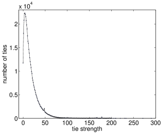
Figure 1: The distribution of the strength of ties, measured as the number of triads each tie participates in.

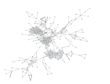
Figure 2: The largest component of the reduction of the BuddyZoo network where each tie participates in at least 47 triads. The triads themselves are not all shown — only the ties that share a threshold number of them.

In order to determine the presence of strong ties, we consider only users who explicitly registered with BuddyZoo, but we allow an edge to be considered transitive if it is part of a closed triad that includes an unregistered user. This is because we know that two people share a contact, even if that contact did not register. We exclude shared contacts that have indegree greater than 1000, because those could be AIM bots (automated response programs). We do not include unregistered contacts in the network itself because their Buddy List information is incomplete. The degree distribution is highly skewed and there are many isolates in the network. On average, each user is connected via a reciprocated tie to 6.83 other registered BuddyZoo users. We require a tie to be reciprocated, since it is possible for one AIM user to add someone to their buddy list without that person adding them in turn.

component size	BuddyZoo	BuddyZoo
		without weak ties
124672	1	0
122066	0	1
21-40	0	1
11-20	11	14
10	4	6
9	5	5
8	7	9
7	7	10
6	15	16
5	37	36
4	64	73
3	126	168
2	591	685
1	7279	9413

Table 2: Distribution of connected components in the BuddyZoo AOL instant messenger community. A tie is considered weak if two users who list each other on their buddy lists do not list a third person in common.

As in the case of the Club Nexus social network, we find that removing weak ties does not have a dramatic effect on the BuddyZoo network. Although several communities containing a couple of dozen nodes do split off, the giant component shrinks modestly, from occupying 88.9% of the graph to occupying 87.5% of it. The average shortest path increases by a fraction of a hop from 7.1 to 7.3. Usually any lengthening in the path decreases the probability of a successful transmission if the probability that the message is transferred at each step is less than 1 watts2002search . However, we do not observe considerable lengthening of the average shortest path until we impose a higher threshold on tie strength.

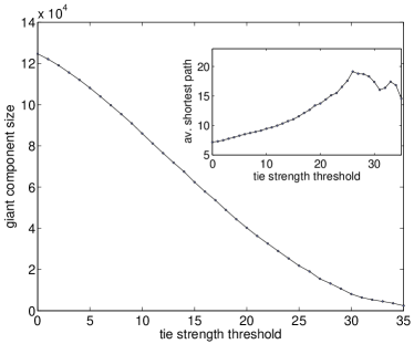
Figure 3: The size of the giant component as only ties of a minimum strength (measured in the number of triads it is a part of) are kept in the network. The inset shows the growth of the average shortest path between connected pairs.

In order to consider more restrictive requirements on tie strength, we vary the strength threshold as follows: rather considering any tie in a single closed triad to be strong, we require that it be part of at least $j$ closed triads. Figure 1 shows the distribution of tie strengths, where the mean number of shared ties is 17.4 and the median is 13. Figure 2 shows the largest component of nodes where each tie participates in at least 47 triads. There are several dense cliques, but the largest component is quite small - only 233 nodes. To investigate how rapidly the giant component shrinks and how much the average shortest distance changes, we consider reduced networks where only ties of above threshold strength, measured by the number of triads the tie participates in, are kept. Figure 3 shows the giant component size and average shortest path between all connected pairs as the threshold is increased from zero to 35 triads. We observe that the giant component shrinks gradually, indicating that a substantial portion of the network is spanned by ties of moderate strength. This would indicate that the network is composed of overlapping communities rather than separate communities that are bridged by weak ties. What is more, removing weak ties does not separate large communities from one another. Rather, a few smaller communities and many isolates are spun off as the tie strength threshold is increased. Removing weak ties has an additional cost beyond isolating some individual nodes and smaller communities — it increases the average shortest path between reachable pairs. So even though the giant component is shrinking, we are removing the shortcuts that span it. The average shortest path more than doubles as we increase the threshold from 1 to 25.

The strong tie robustness of the Club Nexus and BuddyZoo networks is encouraging, especially in comparison to what one might expect in a Watts-Strogatz (WS) type small world model Watts98smallworld or an Erdös-Renyi graph. In the WS model, the network is constructed from a lattice where each node is connected to $k$ neighbors on each side. For $k>1$, this means that each node participates in local closed triads. In the model, a fraction $p$ of the links are rewired with one endpoint placed randomly among the nodes. It is the presence of these random links that gives the WS model a shortest path that scales logarithmically with the size of the graph. Such a link is unlikely to be part of triangle however, since the probability of any two nodes linking randomly is proportional to $1/N$ in such a graph. Therefore, removing weak links in a WS model removes the shortcuts, leaving an average shortest path that scales linearly with the size of the graph. Assuming that nodes close together on the lattice share similar information, one would need to make many hops in order to find novel information. In section III.3, we will show that the occurrence of strong ties in an Erdös-Renyi graph is unlikely unless the average degree increases with the number of nodes in the network. Therefore, removing all edges that are not part of a triangle will isolate most of the nodes in random graphs where the average degree is constant or nearly constant with respect to the number of nodes.

III Model of a random triangle graph

Given the results of the previous section, where we see a very high prevalence of transitive ties and a robustness of the network with respect to removal of weak ties, we seek to answer the basic question of the cost of requiring all ties to be transitive. In order to do this we consider the very simplest model of a random graph where every edge between two nodes is part of at least one closed triad, and investigate some properties of the graph analytically. In essence, the graph is composed entirely of triangles, and we model this kind of graph by assigning links among any three randomly chosen nodes in the graph. Strictly speaking, for a graph with $|V|=N$ nodes, there are $N\choose 3$ possible combinations of nodes that can form a triangle. Each triangle forms with probability $b$, so that on average we randomly choose $M=b\times{N\choose 3}$ triplets of nodes and link them with three edges.

Note that our method of constructing transitive graphs is similar to a particular instance of the Newman Newman03clusterednetworks model for constructing highly clustered graphs. In the Newman clustered network model, one takes a bipartite network of individuals and groups. One then constructs a one-mode projection of the random graph by adding, with a given probability $p$, edges directly between individuals who belong to the same group. However, unlike Newman03clusterednetworks , in our model the probability for nodes to connect to each other in the same group is 1, and the number of members in each group is constant at 3.

III.1 Degree distribution

We consider the degree distribution of the graph starting from the distribution of a node belonging to $k$ closed triads.

For each node $u$, there is a total of $R={N-1\choose 2}$ possible triangles which have $u$ as one of the vertices. And, for each triple of vertices, the probability of being selected to have links in the graph is $b$. Let $r_{m}$ be the probability for a node belong to $m$ chosen triples. Then

$$r_{m}={R\choose m}b^{m}(1-b)^{R-m}.$$ (1)

On the other hand, we will now show that it is unlikely that our fixed node $u$ is part of two triangles with an edge in common. Our node $u$ has degree $k$ if, for some $m$, node $u$ is in $m$ chosen triples on a total of $k$ distinct nodes aside from $u$. It is straightforward to show that $k/2\leq m\leq\binom{k}{2}$. In fact, for even $k\ll N$, most of the probability is in the case $m=k/2$, as we now show. For even $k$, the probability that $u$ has degree $k$ is the probability that $u$ is in exactly $k/2$ chosen triples, adjusted for collisions of edges. Collisions affect the probability of degree $k$ in two ways—$u$ may be in exactly $m=k/2$ triples but a collision reduces the contribution to the probability of degree $k$, or $u$ may be in $m>k/2$ chosen triples but collisions increase the contribution to the probability that the degree is $k$.

Conditioned on $u$ falling in exactly $m$ chosen triples, all sets of $m$ triples are equally likely. There are $\binom{R}{m}=\Theta\left(\frac{N^{2m}}{2^{m}m!}\right)$ possible sets of $m$ triples. Next, we want to count the number of sets of $m$ triples involving exactly $j$ neighbors of $u$, for $j\leq 2m$. We can pick the $j$ neighbors as a set in $\binom{N-1}{j}$ ways, but then we need to assign roles to the $j$ neighbors based on collision multiplicity. For example, suppose 4 triples among five neighbors $A,B,C,D,E$ of $u$ might be $\{u,A,B\},\{u,A,C\},\{u,A,D\},\{u,B,E\}$. We can choose $A,B,C,D,E$ as a set; pick an element for the role of $A$ (that appears three times) in 5 ways; given that, pick an element for the role of $B$ in 4 ways; then $E$ in 3 ways, and the remaining elements take the interchangeable roles of $C$ and $D$, for a total of $5\cdot 4\cdot 3\leq 5!$ orderings).

For us, a crude bound for the orderings of roles will suffice. There are at most $2m-j$ collisions counting multiplicities, and so at most $2m-j$ neighbors of $u$ that can be in more than one triple—play a non-trivial role. There are at most $2m-j$ roles. So the number of ways to assign non-trivial roles is at most $(2m-j)^{2m-j}$. So the number of sets of $m$ triples involving exactly $j$ neighbors of $u$ is at most $\binom{N-1}{j}(2m-j)^{2m-j}$. Thus the ratio of these to the number of sets of $m$ disjoint triples is

$$\frac{\binom{N-1}{j}(2m-j)^{2m-j}}{\binom{R}{m}} \leq O\left(\frac{N^{j}(2m-j)^{2m-j}2^{m}m!}{j!N^{2m}}\right)$$

$$\leq O\left(\frac{((2m-j)/N)^{2m-j}2^{m}m!}{j!}\right).$$

We are intereseted in the case $2m-j\geq 1$. If $m$ and $j$ are constants, then we can ignore $2^{m}m!/j!$, and we get

$$\frac{\binom{N-1}{j}(2m-j)^{2m-j}}{\binom{R}{m}} \leq O\left(\frac{((2m-j)/N)^{2m-j}2^{m}m!}{j!}\right)$$

$$\leq O\left(1/N\right).$$

By choosing the appropriately small probability $b$ of choosing a triple, we may assume that $m$ and $j$ are much smaller than $N$. But we cannot necessarily assume $m$ and $j$ are constants; for example, we may have $m!$ comparable to $N$. We now consider the case where $j$ or $m$ grows (slowly) with $N$, and where $N$ is sufficiently large. If $m\leq j$, then $2^{m}m!/j!\leq\binom{j}{m}^{-1}\leq 1$. It follows that

$$\frac{\binom{N-1}{j}(2m-j)^{2m-j}}{\binom{R}{m}} \leq O\left(\frac{((2m-j)/N)^{2m-j}2^{m}m!}{j!}\right)$$

$$\leq O\left(((2m-j)/N)^{2m-j}\right)$$

$$\leq O(N^{-1}).$$

On the other hand, if $m>j$, then $2m-j>m$, so

$$\frac{\binom{N-1}{j}(2m-j)^{2m-j}}{\binom{R}{m}} \leq O\left(\frac{((2m-j)/N)^{2m-j}2^{m}m!}{j!}\right)$$

$$\leq O\left(((2m-j)/N)^{2m-j}(2m)^{m}\right)$$

$$\leq O\left((2m(2m-j)/N)^{2m-j}\right).$$

If $2m-j=1$, this is $O(2m/N)\leq N^{-1+o(1)}$. If $2m-j>1$, then, since we may assume that $2m\ll\sqrt{N}$, we have

$$\frac{\binom{N-1}{j}(2m-j)^{2m-j}}{\binom{R}{m}} \leq O\left((2m(2m-j)/N)^{2m-j}\right)$$

$$\leq O\left(((2m-j)/\sqrt{N})^{2m-j}\right)$$

$$\leq O\left(((2m-j)^{2}/N)^{(2m-j)/2}\right).$$

This is $O\left((2m-j)^{2}/N\right)\leq N^{-1+o(1)}$.

We conclude that the effect of collisions is small in any case. Thus we get the probability of $u$ having degree $k$ is

$$p_{k}=\left\{\begin{array}[]{ l l }{R\choose{\frac{k}{2}}}b^{\frac{k}{2}}(1-b)^{R-\frac{k}{2}}\pm N^{-1+o(1)}&\mbox{if $k$ is even}\\ N^{-1+o(1)},&\mbox{if $k$ is odd}\\ \end{array}\right.$$ (2)

After ignoring the additive amount $\pm N^{-1+o(1)}$, the corresponding generating function is given by

$$G_{0}(z)=\sum^{R}_{k=0}{R\choose k}b^{k}(1-b)^{R-k}z^{2k}=[bz^{2}+1-b]^{R}$$ (3)

The average degree $\langle k\rangle$ is then given by:

$$\langle k\rangle=G_{0}^{\prime}(1)=b(N-1)(N-2)$$ (4)

And thus, we have the relationship between average degree $\langle k\rangle$ and the probability of any three nodes being connected by a triangle $b$:

$$b=\frac{\langle k\rangle}{(N-1)(N-2)}$$ (5)

When $\langle k\rangle=O(1)$, $b=O\left(\frac{1}{N^{2}}\right)$.

III.2 Accidental triangles and the clustering coefficient

We should notice that in our model, the expected number of triangles in the network is not exactly $b\times{N\choose 3}$. There is the possibility of forming an “accidental” triangle, which can occur when the pairs of nodes $a$ and $b$, $b$ and $c$, and $a$ and $c$ are linked, but the triangle ${a,b,c}$ was not among the $b\times{N\choose 3}$ initially chosen triangles. The probability $b\prime$ of this occurring is the probability that no triangle was intentionally formed between the $a$, $b$, and $c$: $1-b$ times the probability that each of the three edges does occur in a triangle other than ${a,b,c}$.

$$b^{\prime}=(1-b)[1-(1-b)^{(N-3)}]^{3}$$ (6)

In this way, we know that the total expected number of triangles in this graph is $a\times{N\choose 3}$, where $a=b+b^{\prime}$.

Thus, the ratio between the actual number of triangles in the graph and the input number of triangles is:

$$\Delta=\frac{a}{b}=1+\frac{(1-b)[1-(1-b)^{(N-3)}]^{3}}{b}$$ (7)

However, $b^{\prime}$ is very small compared with $b$, when the average degree of a node in the graph is a constant independent of the growth of the total number of nodes $N$. Since we have shown that $b=O(\frac{1}{N^{2}})$, then it is not hard to see that the ratio of the probability for any three nodes to be part of an accidental triangle and the probability for them to be a triangle that is constructed by randomly choosing groups is:

$$\frac{b^{\prime}}{b}=\frac{(1-b)[1-(1-b)^{(N-3)}]^{3}}{b}=O\left(\frac{1}{N}\right)$$ (8)

Thus, we can see that when $N$ is large, and the average degree $\langle k\rangle$ is independent of $N$, then the chance of forming an accidental triangle is quite small compared to the triangles randomly drawn in constructing the model. Figure 4 shows the relation between $b^{\prime}$ and average degree $\langle k\rangle$.

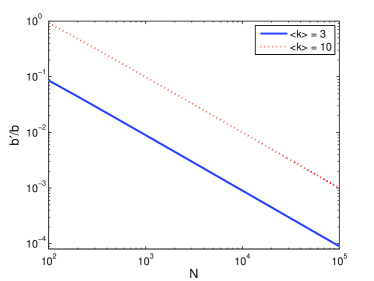
Figure 4: The ratio of the number of accidentally formed triangles to the number randomly chosen by the model. For fixed average degree and increasing number of nodes, the ratio of accidentally formed triangles drops as $1/N$.

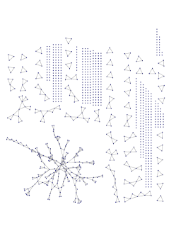
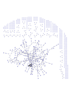
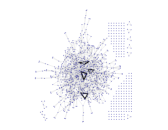
(a) $N=1000$, $M=200$	(b) $N=1000$, $M=300$	(c) $N=1000$, $M=500$

Figure 5: Examples of triangle graphs with 1000 nodes with varying numbers of triangles $M$. Accidental triangles are marked with bold lines.

In Figure 5 we show three instances of a randomly generated graph of triangles. Each graph has $1,000$ nodes, but we form different numbers of triangles. Even though a giant component exists for each graph, it is only once the number of triangles equals the number of nodes that we observe a few random triangles forming. Therefore the formation of accidental triangles does not have a substantial effect on the derivations below.

The clustering coefficient $C$ is a measure of the prevalence of closed triads in a network Watts98smallworld ; newman03structure . The expectation of the total number of connected triples of nodes (open and closed triads) in the graph is $N_{triple}=N\times\sum_{k}{k\choose 2}p_{k}$, and the number of closed triads is $N_{\Delta}\approx b\times{N}{N\choose 3}$ since the number of accidental triangles is small. Thus the clustering coefficient is:

$$C = \frac{3N_{\Delta}}{N_{triple}}$$

$$\approx \frac{3b{N\choose 3}}{N\times\sum_{k}{k\choose 2}p_{k}}$$

$$= O(1)$$

We can see that when $N$ is large, the clustering coefficient of our graph is:

$$C=O(1)$$ (9)

which is significantly larger than the $O(N^{-1})$ clustering coefficient in an Erdös-Renyi Random graph. For many types of real world networks, it has been shown that $C=O(1)$ newman03structure , so it is of interest to see how removing weak ties in real networks changes the clustering coefficients.

III.3 Phase transition and the giant component

For the derivation of the phase transition and size of giant component, we loosely follow the generating function methods for clustered graphs in newman03structure . The phase transition is also known as the percolation threshold - the average degree at which a finite fraction of the network is connected, forming a giant component. In Part A, we have given $r_{m}$, the probability for a node belong to $m$ triangles. Thus, averaging over all individuals and triangles, we have the mean number of triangles a node belongs to: $\mu=\sum_{m}mr_{m}$.

The probability of having two edges within the triangle is 1, and the probability of having any other number is 0. Therefore, the generating function of the number of edges for each node within a triangle is

$$h(z)=z^{2}$$ (10)

Furthermore, for a node $A$ in the graph, the total number of other nodes in the whole graph that it is connected to by virtue of belonging to triangles is generated by:

$$G_{0}(z)=\sum^{\infty}_{m=0}r_{m}(h(z))^{m}$$ (11)

where $r_{m}$ is the probability for a node to belong to $m$ groups as we defined before. This is also the generating function of the distribution of the number of nodes one step away from node $A$.

The generating function of the distribution of the number of nodes two steps away from $A$ is $G_{0}(G_{1}(z))$, where $G_{1}(z)$ is the generating function for the distribution of the number of neighbors of a node arrived at by following an edge (excluding the edge that was used to arrive at the node):

$$G_{1}(z)=\mu^{-1}\sum^{\infty}_{m=0}mr_{m}(h(z))^{m-1}$$ (12)

The necessary and sufficient condition for a giant component to exist, is when, averaging over all the nodes in the graph, the number of nodes two steps away exceeds the number of nodes one step away newman-2001-64 , which can be expressed as:

$$[\partial_{z}(G_{0}(G_{1}(z))-G_{0}(z))]_{z=1}>0$$ (13)

Thus, we get the condition for the existence of a giant component in this graph:

$$((\mu^{-1}\sum^{\infty}_{m=0}m(m-1)r_{m}z^{m-2})\cdot h^{\prime}(z))|_{z=1} > 1$$

$$2\mu^{-1}\sum^{\infty}_{m=0}m(m-1)r_{m} > 1$$

$$\frac{R(R-1)b}{Rb} > \frac{1}{2}$$

After simplifying the above equation, the condition is:

$$b>\frac{1}{N^{2}-3N}$$ (14)

Since we will compare this graph with an Erdös-Renyi random graph with the same average degree $\langle k\rangle$, we express the condition for the existence of giant component in terms of the average degree given by Equation 4:

$$\langle k\rangle>1+\frac{2}{N^{2}-3N}$$ (15)

As $N\rightarrow\infty$, the condition is $\langle k\rangle>1$. An interesting point is that this is exactly where the phase transition occurs in an Erdös-Renyi graph. Therefore, the requirement that all edges be transitive does not delay the appearance of the giant component. It does however have a tempering effect on the rate of growth of the giant component as we will see below.

When a giant component exists in the graph and the probability for a node to whom $A$ is connected to not belong to it is $s$, the size of the giant component is given by:

$$S = 1-G_{0}(s_{0})$$ (16)

$$= 1-\sum^{\infty}_{m=0}r_{m}(s_{0}^{2})^{m}$$ (17)

$$= 1-(bs_{0}^{2}+1-b)^{R}$$ (18)

where $s_{0}$ is the solution of the function:

$$s = G_{1}(s)$$ (19)

$$= \mu^{-1}\sum^{\infty}_{m=0}mr_{m}(s^{2})^{m-1}$$ (20)

$$= (bs^{2}+1-b)^{R-1}$$ (21)

As we have assumed $S>0$, we know that $s$ must be some value larger than 0 and smaller than 1, and thus $s=1$ is a trivial solution of the function.

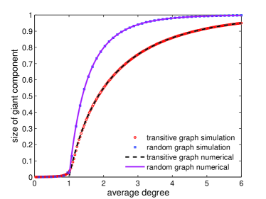
Figure 6: Comparison of numerical simulations with analytical solutions for the fraction of the network occupied by the giant component of a 10,000 node triangle graph and the corresponding Erdös-Renyi graph

We compare the solution $s_{0}$ to numerical simulations of networks of random triangles. Each network contains $N=10,000$ nodes, and we select $M$ random triangles to connect from the $N$ nodes. For each value of $M$ we generate 50 random networks and average the size of the giant component. The results, shown in Figure 6 show excellent agreement between the analytical prediction and the numerical simulation. For comparison, we show both the numerical prediction and analytical result for the size of the giant component in an Erdös-Renyi random graph with the same number of nodes and edges. The size of the giant component in the Erdös-Renyi graph is given by the solution $s$ to the equation $s=1-\exp(-\langle k\rangle s)$. ¿From the figure, we can see that as average degree grows, the phase transitions of the transitive graph and the random graph occur at the same time, while the size of giant component of the Erdös-Renyi graph grows more quickly as we increase the average degree. An intuitive explanation is that in an Erdös-Renyi graph one need not expend a ‘closure’ edge to close a triad. Rather, that edge can be used to connect a disconnected node or small component to the giant component.

The fact that the phase transition occurs at the same average degree for both the Erdös-Renyi and transitive network shows that the requirement of transitivity does not result in a need for increased average connectivity in order for the giant component to form. Note that the phase transition in our model, where all edges are the result of the addition of triangles, is quite different from what it is in a graph that would result from taking a simple Erdös-Renyi graph and removing all edges that do not fall within a triangle. In the Erdös-Renyi graph with non-transitive edge removal the percolation threshold occurs at a degree that scales as $N^{\frac{1}{3}}$.

This condition for the giant component in an Erdös-Renyi graph with weak ties removed can be derived as follows. A giant component of strong tries forms when, after arriving at an arbitrary triangle $T$, the expected value of the number other adjacent triangles that one could“move to” is equal to 1. The probability that there is a triangle $T^{\prime}$ adjacent to $T$ that is not the triangle from which we reached $T$ is given by $2{{N-5}\choose 2}p^{3}$. There are ${{N-5}\choose 2}$ choices for the vertices in $T^{\prime}$ not shared with $T$, and two choices of the vertex shared by $T$ and $T^{\prime}$ (excluding the vertex of $T$ that is shared with the triangle we arrived from). $p=\langle k\rangle/N$ is the probability that any two vertices in an Erdös-Renyi graph share an edge. Thus when $N$ is large, the average degree at the phase transition is $\langle k\rangle=N^{1/3}$. In several real world networks the average degree was found to vary as $N^{\beta}$ where $0\leq\beta\leq 0.3$ leskovec05densification . But in a random network, this density falls short of the $N^{1/3}$ necessary to make the accidental occurrence of closed triads (and therefore strong ties) high enough for the network to percolate.

If one further requires that the triangles overlap not just in one node but in two, as in the percolation of k-cliques derenyi01cliquepercolation , the phase transition occurs at a critical average degree that grows as $N^{\frac{k-2}{k-1}}$, with $k=3$. This means that the average degree has to grow in linear proportion to $N$ in order for a giant component to form. Together, these two results show that the Erdös-Renyi random graph typically does not contain sufficiently numerous strong ties to percolate. But as we have shown in section II, real world social networks do contain many strong ties that percolate. This can be intuitively explained by the observation that new social ties typically form in the context of geographical and sociocultural settings watts2002search . In these contexts it is natural that the ties tend to form closed triads rather than being added independently, as they are in Erdös-Renyi random graphs.

IV Average Shortest Path

Exact results for the average shortest path are difficult to derive even for a random graph. We therefore used numerical simulations to measure the average shortest path between all reachable nodes as we increase the size of the network. We selected a value of the average node degree where the giant component existed, but did not take up all of the graph. At our chosen value, $M=0.5N$, there are twice as many triangles as nodes. This constant proportion of triangles to nodes means that $b$, the probability of any triple of nodes being connected, falls as $1/N^{2}$.

At $M=0.5N$, the giant component occupies 76% of the nodes, while in the equivalent random graph it takes up 94% of the nodes. This makes it difficult to directly compare the two networks, since the average shortest path is measured between reachable pairs, and the Erdös-Renyi graph has more of them. Figure 7 shows that the average shortest path is actually shorter in the triangle graph. This may be explained by the fact that there are fewer nodes in the giant component but a greater density of links. Once we consider the average shortest path relative to the size of the giant component, the curves become nearly identical for both networks. This shows that the requirement of triadic closure does not negatively impact the average shortest path for reachable pairs, but those pairs are fewer in number.

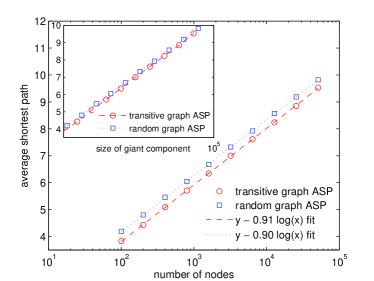
Figure 7: Numerical comparison of the average shortest path in triangle graphs and Erdös-Renyi graphs with the same number of nodes and edges. The inset shows the average shortest path as a function of the size of the giant component rather than the total number of nodes.

V Conclusions and future work

In this paper we study the connectivity of strong ties in networks, where strong ties are defined as belonging to closed triads. We find that two real world social networks are robust with respect to removal of weak links, in the sense that there remains a giant component that is smaller but still occupies a majority of the graph. We also find empirically that the removal of weak links lengthens the average shortest path modestly. In comparison, the removal of weak links in an WS small world network or an Erdös-Renyi graph would isolate the vast majority of nodes. It is the high clustering of social networks that allows them to transmit or gather information via strong ties.

We also pose a basic question, which is the cost paid for the requirement of transitive ties in terms of the size of the giant component and the length of the average shortest path. We consider the simplest random graph model consisting entirely of closed triads and compare it to a network where the links are randomly rewired. We find that the giant component occurs at the same point—when the average node degree equals 1. However, past the phase transition, the giant component in the graph of closed triads grows more slowly than it does in the random network. We further examine the dependence of the average shortest path with the size of the network and find it to be almost identical for reachable pairs in both the triangle graph and the equivalent random network.

An unanswered question is whether more sophisticated models of social structure kleinberg2000navigation ; kleinberg01dynamics ; watts2002search capture the phenomenon of strong ties that can be linked together to span an entire network. In particular, in future work we are interested in examining the strong tie properties of social networks where the edge probabilities depend on the hierarchial organization of underlying social dimensions.

- (1) L. A. Adamic, O. Buyukkokten, and E. Adar. A social network caught in the web. First Monday, 8(6), June 2003.
- (2) D. Cartwright and F. Harrary. A generalizationgeneralization of heider s theory. sychological Review, 63:277–292, 1956.
- (3) Damon Centola and Michael Macy. Complex contagion and the weakness of long ties. ftp://hive.soc.cornell.edu/mwm14/webpage/WLT.pdf.
- (4) I. Derenyi, G. Palla, and T. Vicsek. Clique percolation in random networks. Physical Review Letters, 94:160202, 2005.
- (5) M. S. Granovetter. The strength of weak ties. American Journal of Sociology, 78:1360–1380, 1973.
- (6) R Guimer , B Uzzi, J Spiro, and LAN Amaral. Team assembly mechanisms determine collaboration network structure and team performance. Science, 308:697–702, 2005.
- (7) Tad Hogg and Lada A. Adamic. Enhancing reputation mechanisms via online social networks. In Proceedings of the 5th ACM conference on Electronic Commerce, pages 236–237, June 2004.
- (8) J. Kleinberg. Navigation in a small world. Nature, 406, 2000.
- (9) J. M. Kleinberg. Small-world phenomena and the dynamics of information. In Advances in Neural Information Processing Systems (NIPS), page 14, 2001.
- (10) Jure Leskovec, Jon Kleinberg, and Christos Faloutsos. Graphs over time: Densification laws, shrinking diamaters and possible explanations. In Proceedings of the Eleventh ACM SIGKDD International Conference on Knowledge Discovery and Data Mining, Chicago, IL, 2005. ACM Press.
- (11) M E J Newman. Properties of highly clustered networks. Physical Review E, 68:026121, 2003.
- (12) M.E.J. Newman. The structure and function of complex networks. SIAM Review, 45(2):167–256, 2003.
- (13) M.E.J. Newman, S.H. Strogatz, and D.J. Watts. Random graphs with arbitrary degree distributions and their applications. hysical Review E, 64:026118, 2001.
- (14) Lawrence Page, Sergey Brin, Rajeev Motwani, and Terry Winograd. The pagerank citation ranking: Bringing order to the web. Technical report, Stanford Digital Library Technologies Project, 1998.
- (15) Gergely Palla, Imre Derenyi, Illes Farkas, and Tamas Vicsek. Uncovering the overlapping community structure of complex networks in nature and society. Nature, 814-818:440–442, 2005.
- (16) Filippo Radicchi, Claudio Castellano, Federico Cecconi, Vittorio Loreto, and Domenico Parisi. Defining and identifying communities in networks. PNAS, 101(9):2658–2663, 2004.
- (17) B. Ryan and N.C. Gross. The diffusion of hybrid corn in two iowa communities. Rural Sociology, 8:15–24, 1943.
- (18) David Strang and Sarah A. Soule. Diffusion in organizations and social movements: From hybrid corn to poison pills. Annual Review of Sociology, 24:265–290, 1998.
- (19) D. J. Watts, P. S. Dodds, and M. E. J. Newman. Identity and search in social networks. Science, 296:1302–1305, 2002.
- (20) D. J. Watts and S. H. Strogatz. Collective dynamics of ’small-world’ networks. Nature, 393:440–442, 1998.