Exchange Interaction, Entanglement and Quantum Noise
Due to a Thermal Bosonic Field

Abstract

We analyze the indirect exchange interaction between two two-state systems, e.g., spins $1/2$, subject to a common finite-temperature environment modeled by bosonic modes. The environmental modes, e.g., phonons or cavity photons, are also a source of quantum noise. We analyze the coherent vs noise-induced features of the two-spin dynamics and predict that for low enough temperatures the induced interaction is coherent over time scales sufficient to create entanglement. A nonperturbative approach is utilized to obtain an exact solution for the onset of the induced interaction, whereas for large times, a Markovian scheme is used. We identify the time scales for which the spins develop entanglement for various spatial separations. For large enough times, the initially created entanglement is erased by quantum noise. Estimates for the interaction and the level of quantum noise for localized impurity electron spins in Si-Ge type semiconductors are given.

I Introduction

The idea that exchange of fermionic or bosonic excitations can lead to physical interactions in solid state is not new.Mahan Recently, such induced interactions have received attention due to the possibility to experimentally observe quantum dynamics in nanoscale devices.Jiang ; Jiang2 ; Craig ; Elzerman ; Koppens ; Petta ; MMJ ; PF In this work we explore the dynamics of two qubits (two two-state quantum systems), e.g., electron spins $1/2$, placed a distance $\mathbf{d}$ apart, as they are entangled by common thermalized bosonic environment without direct spatial electron wave function overlap. At the same time quantum noise originating from the same bosonic field (e.g., phonons) ultimately erases the generated entanglement for large enought times. We demonstrate that the indirect exchange interaction induced by the bosonic thermal field STPs can, in some cases, be comparable with other qubit-qubit couplings.

Extensive studies have been reportedBraun ; Eberly1 ; Eberly2 ; Tolkunov1 of the decay of quantum correlations between qubits subject to individual (local) or common environmental noise. In the presence of quantum noise, entanglement was shown to decay very fast and, in some cases, vanish at finite times.Eberly1 ; Eberly2 On the other hand, the idea that common bosonic as well as fermionic environment is able to entangle the qubits has also been advanced.Braun ; STPs ; RKKY ; Bychkov ; PVK ; MPV ; MPG ; Piermarocchi ; Porras ; Mozyrsky ; Rikitake For fermionic environment, this effect has been attributed to Rudermann-Kittel-Kasuya-Yosida (RKKY) type interactionsRKKY ; PVK ; MPV ; MPG ; Piermarocchi ; Mozyrsky ; Rikitake and it has recently been experimentally demonstrated for two-qubit semiconductor nanostructures.Craig ; Elzerman

In this work, we investigate the two competing physical effects of a thermalized bosonic environment (bath) in which two qubits are immersed. Specifically, the induced interaction, which is effectively a zero-temperature effect, and the quantum noise, originating from the same bath modes, are derived within a uniform treatment. We study the dependence of the induced coherent vs noise (decoherence) effects on the parameters of the bath modes, the qubit system, and their coupling, as well as on the geometry. Specific applications are given for spins interacting with phonons in semiconductors.

We assume that the spins are identically coupled with the modes of a thermalized bosonic bath, described by $H_{B}=\sum_{\mathbf{k},\mathbf{\xi}}\omega_{\mathbf{k},\mathbf{\xi}}a_{\mathbf{k},\mathbf{\xi}}^{\dagger}a_{\mathbf{k},\mathbf{\xi}}$, where we introduced the polarization index $\mathbf{\xi}$ and set $\hbar=1$. With qubits represented as spins $1/2$, the external magnetic field is introduced in the qubit Hamiltonian

$$H_{S}=\Delta(\sigma_{z}^{1}+\sigma_{z}^{2})/2,$$ (1.1)

as the energy gap $\Delta$ between the up and down states for spins 1 and 2, with the spins labeled by the superscripts. A natural example of such a system are spins of two localized electrons interacting via lattice vibrations (phonons) by means of the spin-orbit interaction.Mahan ; Hasegawa ; Roth ; SO-Winkler Another example is provided by atoms or ions in a cavity, used as two-state systems interacting with photons. For each type of phonon/photon, the interaction will be assumedMahan ; SO-Winkler ; Leggett ; VKampen linear in the bosonic variables. The spin-boson coupling for two spins $j=1,2$ has the form

$$H_{SB}=\sum\limits_{j=1,2}\sum\limits_{m=x,y,z}\sigma^{j}_{m}X^{j}_{m},$$ (1.2)

where $\sigma^{j}_{m}$ are the standard Pauli matrices and

$$X^{j}_{m}=\sum_{\mathbf{k},\mathbf{\xi}}g^{m}_{\mathbf{k},\mathbf{\xi}}e^{i\mathbf{k}\cdot\mathbf{r}_{j}}\left(a_{\mathbf{k},\mathbf{\xi}}+a_{-\mathbf{k},\mathbf{\xi}}^{\dagger}\right).$$ (1.3)

Here, as before, the index $\xi$ accounts for the polarization and $\mathbf{r}_{j}$ is the position of $j$th spin. The overall system is described by the Hamiltonian $H=H_{S}+H_{B}+H_{SB}$. Our emphasis will be on comparing the relative importance of the coherent vs. noise effects of a given bosonic bath in the two-qubit dynamics. We do not include other possible two-qubit interactions in such comparative calculation of dynamical quantities.

For the analysis of the induced exchange interaction and quantum noise for most time scales of relevance, it is appropriate to use the Markovian approachVKampen ; Louisell ; Blum that assumes instantaneous rethermalization of the bath modes. In Section II, we derive in a unified formulation the bath-induced spin-spin interaction and noise terms in the dynamical equation for the spin density matrix. The onset of the interaction for very short times is also investigated within an exactly solvable model presented in Sections III and IV. Specifically, in Section IV, we discuss the onset and development of the interaction Hamiltonian, as well as the density matrix. It is shown that the initially unentangled spins can develop entanglement. We find that the degree of the entanglement and the time scale of its ultimate erasure due to noise can be controlled by varying several parameters, as further discussed for various bath types in Section V. Estimates for the induced coherent interaction in Si-Ge type semiconductors are presented in Section VI. The coherent interaction induced by phonons is, expectedly, quite weak. However, we find that in strong magnetic fields it can become comparable with the dipole-dipole coupling.

II Coherent Interaction and Quantum Noise Induced by Thermalized Bosonic Field

In this section we present the expressions for the induced interaction and also for the noise effects due to the bosonic environment, calculated perturbatively to the second order in the spin-boson interaction, and with the assumption that the environment is constantly reset to thermal. Specific applications and examples are considered towards the end of this section, as well as in Sections V and VI.

The dynamics of the system can be described by the equation for the density matrix

$$i\dot{\rho}(t)=[H,\rho(t)].$$ (2.1)

In order to trace over the bath variables, we carry out the second-order perturbative expansion. This dynamical description is supplemented by the Markovain assumptionLeggett ; VKampen ; Louisell ; Blum of resetting the bath to thermal equilibrium, at temperature $T$, after each infinitesimal time step, as well as at time $t=0$, thereby decoupling the qubit system from the environment.Leggett ; VKampen This is a physical assumption appropriate for all but the shortest time scales of the system dynamics.Privman ; Tolkunov2 ; Solenov It can also be viewed as a means to phenomenologically account in part for the randomization of the bath modes due to their interactions with each other (anharmonicity) in real systems. This leads to the master equation for the reduced density matrix of the qubits $\rho_{S}(t)=Tr_{B}\rho(t)$,

$$i\dot{\rho}_{S}(t) = [H_{S},\rho_{S}(t)]$$

$$- i\int\limits_{0}^{\infty}{dt^{\prime}Tr_{B}[H_{SB},[H_{SB}(t^{\prime}-t),\rho_{B}\rho_{S}(t)]]},$$

where $H_{SB}(\tau)=e^{i(H_{B}+H_{S})\tau}H_{SB}e^{-i(H_{B}+H_{S})\tau}$, $\rho_{B}=\mathrm{Z}^{-1}\prod_{k}e^{-\omega_{k}a_{k}^{\dagger}a_{k}/k_{B}T}$, and $\mathrm{Z}=1/\prod_{k}(1-e^{-\omega_{k}/k_{B}T})$ is the partition function. Analyzing the structure of the integrand in Eq.(II), one can obtain the equation with explicitly separated coherent and noise contributions, see Appendix A,

$$i\dot{\rho}_{S}(t)=[H_{\textrm{eff}},\rho_{S}(t)]+i{\hat{M}}\rho_{S}(t).$$ (2.3)

Here the effective coherent Hamiltonian $H_{\textrm{eff}}$ is

$$H_{\textrm{eff}}\!\!\! = \!\!\!H_{S}+\!\!\!\sum\limits_{m=x,y,z}\!\!\!{2\chi_{c}^{m}({\mathbf{d}})\sigma_{m}^{1}\sigma_{m}^{2}}-\chi_{s}^{x}({\mathbf{d}})\left({\sigma_{x}^{1}\sigma_{y}^{2}+\sigma_{x}^{2}\sigma_{y}^{1}}\right)$$

$$+ \!\!\!\chi_{s}^{y}({\mathbf{d}})\left({\sigma_{y}^{1}\sigma_{x}^{2}+\sigma_{y}^{2}\sigma_{x}^{1}}\right)-\left[\eta_{s}^{x}(0)+\eta_{s}^{y}(0)\right]\left({\sigma_{z}^{1}+\sigma_{z}^{2}}\right).$$

The expressions for the amplitudes $\chi_{c}^{m}(\mathbf{d})$, $\chi_{s}^{m}(\mathbf{d})$, $\eta_{c}^{m}(\mathbf{d})$, and $\eta_{s}^{m}(\mathbf{d})$ will be given shortly. The first three terms following $H_{S}$ constitute the interaction between the two spins. We will argue below that the leading induced exchange interaction is given by the first added term, proportional to $\chi_{c}^{m}(\mathbf{d})$. The last term corrects the energy gap for each qubit, representing their Lamb shifts.

The explicit expression for the noise term is very cumbersome. It can be represented concisely by introducing the noise superoperator $\hat{M}$, which involves single-qubit contributions, which are usually dominant, as well as two-qubits terms

$${\hat{M}}=\sum\limits_{m,i}\Big{[}{\hat{M}}_{m}^{i}(0)+\sum_{j\neq i}{\hat{M}}_{m}^{ij}(\mathbf{d})\Big{]},$$ (2.5)

where the summations are over the components, $m=x,y,z$, and the qubits, $i,j=1,2$. The quantities entering Eq.(2.5) can be written in terms of the amplitudes $\chi_{s}^{m}(\mathbf{d})$, $\eta_{c}^{m}(\mathbf{d})$, and $\eta_{s}^{m}(\mathbf{d})$, in a compact form, by introducing the superoperators ${\hat{L}}_{a}(O_{1})O_{2}=\{O_{1},O_{2}\}$, ${\hat{L}}(O_{1},O_{2})O_{3}=O_{1}O_{3}O_{2}$, and ${\hat{L}}_{\pm}(O_{1},O_{2})={\hat{L}}(O_{1},O_{2})\pm{\hat{L}}(O_{2},O_{1})$,

$${\hat{M}}_{m}^{ij}(\mathbf{d}) = \eta_{c}^{m}(\mathbf{d})\left[{2{\hat{L}}(\sigma^{i}_{m},\sigma^{j}_{m})-{\hat{L}}_{a}(\sigma^{i}_{m}\sigma^{j}_{m})}\right]$$

$$+ \eta_{s}^{m}(\mathbf{d})\left[{{\hat{L}}_{+}(\sigma^{i}_{m},\varsigma^{j}_{m})-{\hat{L}}_{a}(\sigma^{i}_{m}\varsigma^{j}_{m})}\right]$$

$$- i\chi_{s}^{m}(\mathbf{d}){\hat{L}}_{-}(\sigma^{i}_{m},\varsigma^{j}_{m}),$$

where we defined $\varsigma^{j}_{m}=\frac{i}{2}[\sigma_{z}^{j},\sigma_{m}^{j}]$ and

$${\hat{M}}_{m}^{j}(0) = \eta_{c}^{m}(0)\left[{2{\hat{L}}(\sigma_{m}^{j},\sigma_{m}^{j})-{\hat{L}}_{a}(\sigma_{m}^{j}\sigma_{m}^{j})}\right]$$

$$+ \eta_{s}^{m}(0){\hat{L}}_{+}(\sigma_{m}^{j},\varsigma^{j}_{m})$$

$$- i\chi_{s}^{m}(0)\left[{{\hat{L}}_{-}(\sigma_{m}^{j},\varsigma^{j}_{m})+{\hat{L}}_{a}(\sigma_{m}^{j}\varsigma^{j}_{m})}\right].$$

The amplitudes in Eqs.(LABEL:eq:S2:H-eff, II, II), calculated for the interaction defined in Eqs.(1.2, 1.3), are

$$\chi_{c}^{m}({\mathbf{d}})=-\sum\limits_{\mathbf{\xi}}{\int\limits_{-\infty}^{\infty}{\frac{{Vd{\mathbf{k}}}}{{\left({2\pi}\right)^{3}}}}}\left|{g_{{\mathbf{k}},\mathbf{\xi}}^{m}}\right|^{2}\frac{{\omega_{{\mathbf{k}},\mathbf{\xi}}\cos\left({{\mathbf{k}}\cdot{\mathbf{d}}}\right)}}{{\omega_{{\mathbf{k}},\mathbf{\xi}}^{2}-\Delta^{2}(1-\delta_{m,z})}},$$ (2.8)

$$\eta_{c}^{m}({\mathbf{d}}) = \frac{\pi}{2}\sum\limits_{\mathbf{\xi}}{\int\limits_{-\infty}^{\infty}{\frac{{Vd{\mathbf{k}}}}{{\left({2\pi}\right)^{3}}}}}\left|{g_{{\mathbf{k}},\mathbf{\xi}}^{m}}\right|^{2}\coth\frac{{\omega_{{\mathbf{k}},\mathbf{\xi}}}}{{2k_{\textrm{B}}T}}\cos\left({{\mathbf{k}}\cdot{\mathbf{d}}}\right)$$ (2.9)

$$\times \sum\limits_{q=\pm 1}{\delta\left({\omega_{{\mathbf{k}},\mathbf{\xi}}+(1-\delta_{m,z})q\Delta}\right)},$$

and

$$\chi_{s}^{m}({\mathbf{d}}) = -\left({1-\delta_{m,z}}\right)\sum\limits_{\mathbf{\xi}}{\int\limits_{-\infty}^{\infty}{\frac{{Vd{\mathbf{k}}}}{{\left({2\pi}\right)^{3}}}}}\left|{g_{{\mathbf{k}},\mathbf{\xi}}^{m}}\right|^{2}\cos\left({{\mathbf{k}}\cdot{\mathbf{d}}}\right)$$ (2.10)

$$\times \sum\limits_{q=\pm 1}{\frac{{\pi s}}{2}\delta\left({\omega_{{\mathbf{k}},\mathbf{\xi}}+q\Delta}\right)},$$

$$\eta_{s}^{m}({\mathbf{d}}) = \left({1-\delta_{m,z}}\right)$$

$$\times \sum\limits_{\mathbf{\xi}}{\int\limits_{-\infty}^{\infty}{\frac{{Vd{\mathbf{k}}}}{{\left({2\pi}\right)^{3}}}}}\left|{g_{{\mathbf{k}},\mathbf{\xi}}^{m}}\right|^{2}\coth\frac{{\omega_{{\mathbf{k}},\mathbf{\xi}}}}{{2k_{\textrm{B}}T}}\frac{{\Delta\cos\left({{\mathbf{k}}\cdot{\mathbf{d}}}\right)}}{{\omega_{{\mathbf{k}},\mathbf{\xi}}^{2}-\Delta^{2}}}.$$

Here the principal values of integrals are assumed.

Note that $\chi_{c}^{m}({\mathbf{d}})$ appears only in the induced interaction Hamiltonian in Eq.(LABEL:eq:S2:H-eff), whereas $\eta_{c}^{m}({\mathbf{d}})$, $\chi_{s}^{m}({\mathbf{d}})$, and $\eta_{s}^{m}({\mathbf{d}})$ enter both the interaction and noise terms. Therefore, in order to establish that the induced interaction can be significant for some time scales, we have to demonstrate that $\chi_{c}^{m}({\mathbf{d}})$ can have a much larger magnitude than the maximum of the magnitudes of $\eta_{c}^{m}({\mathbf{d}})$, $\chi_{s}^{m}({\mathbf{d}})$, and $\eta_{s}^{m}({\mathbf{d}})$. The third and fourth terms in expression for the interaction (LABEL:eq:S2:H-eff) are comparable to the noise and therefore have no significant contribution to the coherent dynamics.

Because of the complexity of the expressions for the noise terms within the present Markovian treatment, in this section we will only compare the magnitudes of the coherent vs noise effects. In the next section, we will discuss a different model for the noise which will allow a more explicit investigation of the time dependence.

For the rest of this section, we will consider an illustrative one-dimensional (1D) example favored by recent experiments,Craig ; Elzerman leaving the derivations for higher dimensions to Sections V and VI. We comment that the 1D geometry is also natural for certain ion-trap quantum-computing schemes, in which ions in a chain are subject to Coulomb interaction, developing a variety of phonon-mode lattice vibrations.Porras ; Marquet ; Leibfried

In 1D geometry we allow the phonons to propagate in a single direction, along $\mathbf{d}$, so that ${\mathbf{k}}\cdot{\mathbf{d}}=k\left|{\mathbf{d}}\right|$. Here, for definiteness, we also assume the linear dispersion, $\omega_{k}=c_{s}k$, since the details of the dispersion relation for larger frequencies usually have little effect on the decoherence properties. Furthermore, we ignore the polarization, $g_{{\mathbf{k}},\mathbf{\xi}}^{m}\to g^{m}(\omega)$. Another reason to focus on the low-frequency modes is that an additional cutoff $\omega_{c}$ resulting from the localization of the electron wave functions, typically much smaller than the Debye frequency, will be present due to the factors $g^{m}(\omega)$. The induced interaction and noise terms depend on the amplitudes $\chi_{c}^{m}({\mathbf{d}})$, $\eta_{c}^{m}({\mathbf{d}})$, $\chi_{s}^{m}({\mathbf{d}})$, and $\eta_{s}^{m}({\mathbf{d}})$, two of which can be evaluated explicitly for the 1D case, because of the $\delta$-functions in Eqs.(2.9, 2.10). However, to derive an explicit expression for $\chi_{c}^{m}({\mathbf{d}})$ and $\eta_{s}^{m}({\mathbf{d}})$, one needs to specify the $\omega$-dependence in $\left|{g^{m}(\omega)}\right|^{2}$. For the sake of simplicity, in this section we approximate $|g^{m}(\omega)|^{2}$ by a linear function with superimposed exponential cutoff. For a constant 1D density of states $\Upsilon(\omega)=V/2\pi c_{s}$, this is the Ohmic-dissipation condition,Leggett i.e.,

$$|g^{m}(\omega)|^{2}\Upsilon(\omega)=\alpha^{m}_{n}\omega^{n}\exp(-\omega/\omega_{c}),$$ (2.12)

with $n=1$ (the case when $n>1$ is considered in Section V).

In most practical applications, we expect that $\Delta\ll\omega_{c}$. With this assumption, we obtain

$$\chi_{c}^{m}({\mathbf{d}})=\frac{{\alpha_{1}^{m}\omega_{c}}}{{1+\left({{{\omega_{c}\left|{\mathbf{d}}\right|}\mathord{\left/{\vphantom{{\omega_{c}\left|{\mathbf{d}}\right|}{c_{s}}}}\right.\kern-1.2pt}{c_{s}}}}\right)^{2}}},$$ (2.13)

$$\chi_{s}^{m}({\mathbf{d}})=\alpha_{1}^{m}\omega_{c}\frac{\pi}{2}\left({1-\delta_{m,z}}\right)\frac{\Delta}{{\omega_{c}}}\cos\frac{{\Delta\left|{\mathbf{d}}\right|}}{{c_{s}}},$$ (2.14)

and

$$\eta_{c}^{m}({\mathbf{d}})=\alpha_{1}^{m}\omega_{c}\frac{\pi}{2}\left({1-\delta_{m,z}}\right)\frac{\Delta}{{\omega_{c}}}\coth\frac{\Delta}{{2k_{\textrm{B}}T}}\cos\frac{{\Delta\left|{\mathbf{d}}\right|}}{{c_{s}}}.$$ (2.15)

The expression for $\eta_{s}({\mathbf{d}})$ could not be obtained in closed form. However, numerical estimates suggest that $\eta_{s}({\mathbf{d}})$ is comparable to $\eta_{c}^{m}({\mathbf{d}})$. At short spin separations $\mathbf{d}$, $\eta_{s}({\mathbf{d}})$ is approximately bounded by $-\alpha_{1}^{m}\Delta\ln\frac{\Delta}{\omega_{c}}\exp(-\frac{{\Delta\left|{\mathbf{d}}\right|}}{{c_{s}}})$, while at lager distances it may be approximated by $\alpha_{1}^{m}\Delta\frac{\pi}{2}\sin\frac{{\Delta\left|{\mathbf{d}}\right|}}{{c_{s}}}\coth\frac{\Delta}{2k_{\textrm{B}}T}$. The level of noise may be estimated by considering the quantity

$${\cal M}=\max_{|\mathbf{d}|}\left|{\eta_{c}^{m}(\mathbf{d}),\chi_{s}^{m}(\mathbf{d}),\eta_{s}^{m}(\mathbf{d})}\right|.$$ (2.16)

The interaction Hamiltonian takes the form

$$H_{\operatorname{int}}=-\frac{2}{{1+\left({{{\omega_{c}\left|{\mathbf{d}}\right|}/{c_{s}}}}\right)^{2}}}\sum\limits_{m=x,y,z}{\alpha_{1}^{m}\omega_{c}\sigma_{m}^{1}\sigma_{m}^{2}}.$$ (2.17)

This induced interaction is temperature independent. It is long-range and decays as a powerlaw for large $\mathbf{d}$. For the super-Ohmic case, $n>1$, one obtains similar behavior, except that the interaction decays as a higher negative power of $\mathbf{d}$, as will be shown in Section V.

If the noise term were not present, the spin system would be governed by the Hamiltonian $H_{S}+H_{\textrm{int}}$. To be specific, let us analyze the spectrum, for instance, for $\alpha_{1}^{x}=\alpha_{1}^{y}$, $\alpha_{1}^{z}=0$. The two-qubit states consist of the singlet $(\left|{\uparrow\downarrow}\right\rangle-\left|{\downarrow\uparrow}\right\rangle)/\sqrt{2}$ and the split triplet $\left|{\uparrow\uparrow}\right\rangle$, $(\left|{\uparrow\downarrow}\right\rangle+\left|{\downarrow\uparrow}\right\rangle)/\sqrt{2}$, and $\left|{\downarrow\downarrow}\right\rangle$, with energies $E_{2}=-4\chi_{c}^{x}$, $E_{0}=-\Delta$, $E_{1}=4\chi_{c}^{x}$, $E_{3}=\Delta$, respectively. The energy gap $|E_{1}-E_{2}|$ between the two entangled states is defined by $4\chi_{c}^{x}$ ($=4\chi_{c}^{y}$). In the presence of noise, the oscillatory, approximately coherent evolution of the spins can be observed over several oscillation cycles provided that $2\alpha_{1}^{m}\omega_{c}/[1+(\omega_{c}|\mathbf{d}|/c_{s})^{2}]>{\cal M}$. The energy levels will acquire effective width due to quantum noise, of order $\eta_{c}^{m}(\mathbf{d})$. This interplay between the interaction and noise effects is further explored within an exactly solvable model in the next section.

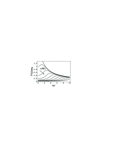
Figure 1: Short-time correction to the induced exchange interaction for the Ohmic case. The arrow shows the order of the curves for increasing $\omega_{c}|\mathbf{d}|/c_{s}=0,1,...,10$.

III Exactly Solvable Model

In this section, we consider a model appropriate for short times,Privman ; Tolkunov2 ; Solenov which does not invoke the Markovian assumption of the rethermalization of the bath modes. This model is particularly suitable for investigating the onset of the system’s dynamics. While the noise effects are quantitatively different in this model, the qualitative interplay of the coherent and noise effects in the dynamics is the same as in the Markovian approach. Furthermore, we will show that the induced interaction is consistent with the one obtained within Markovian approach in the previous section.

We point out that, due to the instantaneous rethermalization assumption (resetting the density matrix of the bath to thermal), in the Markovain formulation it was quite natural to assume that the bath density matrix is also thermal at time $t=0$; the total density matrix retained an uncorrelated-product form at all times. In the context of studying the short-time dynamics, in this section the choice of the initial condition must be addressed more carefully. In quantum computing applications, the initially factorized initial condition has been widely used for the qubit-bath systemPrivman ; Tolkunov2 ; Solenov

$$\rho(0)=\rho_{S}(0)\rho_{B}(0).$$ (3.1)

This choice allows comparison with the Markovian results, and is usually needed in order to make the short-time approximation schemes tractable,Solenov specifically, it is necessary for exact solvability of the model considered in this and the next sections.

A somewhat more “physical” excuse for factorized initial conditions has been the following. Quantum computation is carried out over a sequence of time intervals during which various operations are performed on individual qubits and on pairs of qubits. These operations include control gates, measurement, and error correction. It is usually assumed that these “control” functions, involving rather strong interactions with external objects, as compared to interactions with sources of quantum noise, erase the fragile entanglement with the bath modes that qubits can develop before those time intervals when they are “left alone” to evolve under their internal (and bath induced) interactions. Thus, for evaluating relative importance of the quantum noise effects on the internal (and bath induced) qubit dynamics, which is our goal here, we can assume that the state of qubit-bath system is “reset” to uncorrelated at $t=0$.

It turns out that the resulting model is exactly solvable for the Zeeman splitting $\Delta=0$, and provided that only a single system operator enters the expression (1.2) for the interaction. Here we take $\alpha_{n}^{y}=\alpha_{n}^{z}=0$, while $\alpha_{n}^{x}\neq 0$. We derive the exact solution and demonstrate the emergence of the interaction (2.17).

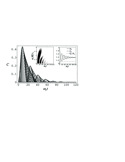
Figure 2: Development of the concurrence as a function of time, calculated with $\alpha^{x}_{1}=1/20$ and $k_{\textrm{B}}T/\omega_{c}=1/20$. The curves correspond to various spin-spin separations, as can be read off the left inset, which shows the distribution of the concurrence in the $|\mathbf{d}|$-$t$ plane. The right inset presents the dynamics of the diagonal density matrix elements $P_{\uparrow\uparrow}\equiv\langle\uparrow\uparrow|\rho_{S}|\uparrow\uparrow\rangle$, etc., on the same time scale.

With the above assumptions, one can utilize the bosonic operator techniquesLouisell to obtain the reduced density matrix for the system (1.2, 1.3),

$$\rho_{S}(t)=\sum\limits_{\lambda,\lambda^{\prime}}{P_{\lambda}\rho_{S}(0)P_{\lambda^{\prime}}e^{\mathfrak{L}_{\lambda\lambda^{\prime}}(t)}},$$ (3.2)

where the projection operator is defined as $P_{\lambda}=\left|{\lambda_{1}\lambda_{2}}\right\rangle\left\langle{\lambda_{1}\lambda_{2}}\right|$, and $\left|{\lambda_{j}}\right\rangle$ are the eigenvectors of $\sigma_{x}^{j}$. The exponent in Eq.(3.2) consists of the real part, which leads to decay of off-diagonal density-matrix elements resulting in decoherence,

$$\textrm{Re}\mathfrak{L}_{\lambda\lambda^{\prime}}(t) = \!\!-\!\!\sum\limits_{k}{G_{k}(t,T)\left[{\left({\lambda^{\prime}_{1}-\lambda_{1}}\right)^{2}+\left({\lambda^{\prime}_{2}-\lambda_{2}}\right)^{2}}\right.}$$ (3.3)

$$+ \!\!\!\left.{2\cos\!\left({\frac{{\omega_{k}\left|{\mathbf{d}}\right|}}{{c_{s}}}}\right)\!\left({\lambda^{\prime}_{1}-\lambda_{1}}\right)\left({\lambda^{\prime}_{2}-\lambda_{2}}\right)}\right]$$

and the imaginary part, which describes the coherent evolution,

$$\textrm{Im}\mathfrak{L}_{\lambda\lambda^{\prime}}(t)=\sum\limits_{k}{C_{k}(t)\cos\left({\frac{{\omega_{k}\left|{\mathbf{d}}\right|}}{{c_{s}}}}\right)\left({\lambda_{1}\lambda_{2}-\lambda^{\prime}_{1}\lambda^{\prime}_{2}}\right)}.$$ (3.4)

Here we defined the standard spectral functionsLeggett ; Privman

$$G_{k}(t,T)=2\frac{{\left|{g_{k}}\right|^{2}}}{{\omega_{k}^{2}}}\sin^{2}\left(\frac{{\omega_{k}t}}{{2}}\right)\coth\left({\omega_{k}\over 2k_{B}T}\right)$$ (3.5)

and

$$C_{k}(t)=2\frac{{\left|{g_{k}}\right|^{2}}}{{\omega_{k}^{2}}}\left({\omega_{k}t-\sin\omega_{k}t}\right).$$ (3.6)

Calculating the sums by converting them to integrals over the bath-mode frequencies $\omega$ in Eqs.(3.3) and (3.4), assuming the Ohmic bath $n=1$ for $T>0$ one obtains a linear in time $t$ large-time behavior for both the temperature-dependent real part and for the imaginary part. The coefficient for the former is $\sim\!kT$, whereas for the latter it is $\sim\!\omega_{c}$. For super-Ohmic models, $n>1$, the real part grows slower, as was also noted in the literature.VKampen ; Privman ; PALMA

Let us first analyze the effect that the imaginary part of $\mathfrak{L}_{\lambda\lambda^{\prime}}(t)$ has on the evolution of the reduced density matrix, since this contribution leads to the induced interaction. If the real part were not present, i.e., omitting Eq.(3.3) from Eqs.(3.2), (3.4), and (3.6), we would obtain the evolution operator in the form $\exp[-iH_{\textrm{int}}t-iF(t)t]$. The interaction $H_{\textrm{int}}$ comes from the first term in Eq.(3.6),

$$H_{\textrm{int}}\!=\!-\frac{2\alpha_{n}^{x}\Gamma(n)c_{s}^{n}\omega_{c}^{n}}{\left(c_{s}^{2}+\omega_{c}^{2}\left|{\mathbf{d}}\right|^{2}\right)^{n/2}}\cos\left[{n\arctan\left({\frac{{\omega_{c}\left|{\mathbf{d}}\right|}}{{c_{s}}}}\right)}\right]\!\sigma_{x}^{1}\sigma_{x}^{2}.$$ (3.7)

This expression is the same as the results obtained within the Markovian scheme, cf., Eqs.(2.17), (2.8), and Section V. The operator $F(t)$ is given by

$$F(t)=2\sigma_{x}^{1}\sigma_{x}^{2}\int\limits_{0}^{\infty}{d\omega\frac{{D(\omega)\left|{g(\omega)}\right|^{2}}}{\omega}\frac{{\sin\omega t}}{{\omega t}}\cos\left(\frac{\omega|\mathbf{d}|}{c_{s}}\right)}.$$ (3.8)

It commutes with $H_{\textrm{int}}$ and therefore could be viewed as the initial time-dependent correction to the interaction. In fact, it describes the onset of the induced coherent interaction; note that $F(0)=-H_{\textrm{int}}$, but for large times $F(t)\sim\alpha^{x}_{n}\omega_{c}^{n}/(\omega_{c}t)^{n}$. In Figure 1, we plot ${\cal F}(t)$, defined via $F(t)={\cal F}(t)\sigma_{x}^{1}\sigma_{x}^{2}$, for the Ohmic case as a function of time for various spin-spin separations.

Let us now explore the role of the decoherence term (3.3). In the exact solution of the short-time model, the bath is thermalized only initially, while in the perturbative Markovian approximation, one assumes that the bath is reset to thermal after each infinitesimal time step. Nevertheless, the effect of the noise is expected to be qualitatively similar. Since the short-time model offers an exact solution, we will use it to compare the coherent vs noise effects in the two-spin dynamics. We evaluate the concurrence,Wootters1 ; Wootters2 which measures the entanglement of the spin system and is monotonically related to the entanglement of formation.Bennett ; Vedral For a mixed state of two qubits, $\rho_{S}$, we first define the spin-flipped state, $\tilde{\rho}_{S}=\sigma^{1}_{y}\sigma^{2}_{y}\,\rho^{*}_{S}\,\sigma^{1}_{y}\sigma^{2}_{y}$, and then the Hermitian operator $R=\sqrt{\sqrt{\rho_{S}}\tilde{\rho}_{S}\sqrt{\rho_{S}}}$, with eigenvalues $\lambda_{i=1,2,3,4}$. The concurrence is then givenWootters2 by

$$C\left({\rho_{S}}\right)=\max\left\{{0,2\mathop{\max}\limits_{i}\lambda_{i}-\sum\limits_{j=1}^{4}{\lambda_{j}}}\right\}.$$ (3.9)

In Figure 2, we plot the concurrence as a function of time and the spin-spin separation, for the (initially unentangled) state $\left|\uparrow\uparrow\right\rangle$, and $n=1$. One observes decaying periodic oscillations of entanglement. We should point out that the measure of entanglement we use here — the concurrence — provides the estimate of how much entanglement can be constructed provided the worst possible scenario for decomposing the density matrix is realized; see Refs. Wootters1, , Wootters2, for details and definitions. Therefore, one expects the entanglement that one can make use of in quantum computing to be no smaller than the one presented in Figure 2. In the next section, additional quantities are considered, namely, the density matrix elements, which characterize the degree of coherence in the system’s dynamics.

IV Onset of the interaction and dynamics of the density matrix

Let us now investigate in greater detail the onset of the induced interaction, the time-dependence of which is given by $F(t)$. In Figure 1 we have shown the magnitude of $F(t)$, as a function of time for various qubit-qubit separations and $n=1$. The correction is initially nonmonotonic, but decreases for larger times as mentioned above. The behavior for other non-Ohmic regimes is initially more complicated, however the large time behavior is similar.

It may be instructive to consider the time dependent correction $H_{F}(t)$ to the interaction Hamiltonian during the initial evolution, corresponding to $F(t)$. Since $F(t)$ commutes with itself at different times, as well as with $H_{\textrm{\footnotesize int}}$, it generates unitary evolution according to $\exp[-i\int_{0}^{t}dt^{\prime}H_{F}(t^{\prime})]$, with $H_{F}(t)=d[tF(t)]/dt$, therefore

$$H_{F}(t) = \sigma_{x}^{1}\sigma_{x}^{2}\alpha_{n}\Gamma(n)$$

$$\times [u(\omega_{c}|\mathbf{d}|/c_{s}-\omega_{c}t)+u(\omega_{c}|\mathbf{d}|/c_{s}+\omega_{c}t)],$$

where $u(\xi)=\cos[n\arctan(\xi)]/[1+\xi^{2}]^{n/2}$. The above expression is a superposition of two waves propagating in opposite directions. In the Ohmic case, $n=1$, the shape of the wave is simply $u(\xi)=1/(1+\xi^{2})$. In Figure 3, we present the amplitude of $H_{F}(t)$, defined via $H_{F}(t)={\cal H}_{F}\sigma_{x}^{1}\sigma_{x}^{2}$, as well as the sum of $H_{\textrm{\footnotesize int}}$ and $H_{F}(t)$, for $n=1$. One can observe that the “onset wave” of considerable amplitude and of shape $u(\xi)$ propagates once between the qubits, “switching on” the interaction. It does not affect the qubits once the interaction has set in.

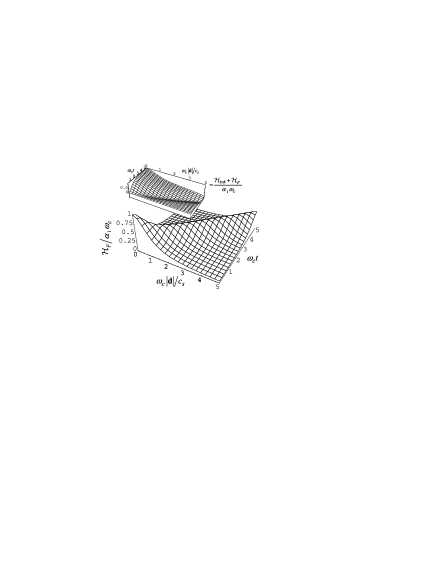
Figure 3: The magnitude of the time-dependent Hamiltonian corresponding to the initial correction as a function of time and distance. The Ohmic ($n=1$) case is shown. The inset demonstrates the onset of the cross-qubit interaction on the same time scale.

To understand the dynamics of the qubit system and its entanglement, let us again begin with the analysis of the coherent part in Eq.(3.2). After the interaction, $H_{\textrm{\footnotesize int}}$, has set in, it will split the system energies into two degenerate pairs $E_{0}=E_{1}=-{\cal H}_{\textrm{\footnotesize int}}$ and $E_{2}=E_{3}={\cal H}_{\textrm{\footnotesize int}}$. The wave function is then $|\psi(t)\rangle=\exp(-iH_{\textrm{\footnotesize int}}t)|\psi(0)\rangle$. For the initial “up-up” state, $|\psi(0)\rangle=\left|\uparrow\uparrow\right\rangle$, it develops as $\left|\psi(t)\right\rangle=\left|\uparrow\uparrow\right\rangle\cos{\cal H}_{\textrm{\footnotesize int}}t+\left|\downarrow\downarrow\right\rangle i\sin{\cal H}_{\textrm{\footnotesize int}}t$, where $H_{\textrm{\footnotesize int}}={\cal H}_{\textrm{\footnotesize int}}\sigma^{1}_{m}\sigma^{2}_{m}$. One can easily notice that at times $t_{E}=\pi/4{\cal H}_{\textrm{\footnotesize int}},3\pi/4{\cal H}_{\textrm{\footnotesize int}},\ldots$, maximally entangled (Bell) states are obtained, while at times $t_{0}=0,\pi/2{\cal H}_{\textrm{\footnotesize int}},\pi/{\cal H}_{\textrm{\footnotesize int}},\ldots$, the entanglement vanishes; these special times can also be seen in Figure 2. The coherent dynamics obtained with the Markovian assumption is the same.

However, the coherent dynamics just described is only approximate, because the bath also induces decoherence that enters via Eq.(3.3). The result for the entanglement is that the decaying envelope function is superimposed on the coherent ocsillations described above. The magnitudes of the first and subsequent peaks of the concurrence are determined only by this function. As temperature increases, the envelope decays faster resulting in lower values of the concurrence; see the inset in Figure 2. Although in the Markovian approach, presented in Section II, the noise is quantitatively different, one expects qualitatively similar results for the dynamics of entanglement.

Note also that nonmonotonic behavior of the entanglement is possible only provided that the initial state is a superposition of the eigenvectors of the induced interaction with more than one eigenvalue (for pure initial states); see Eqs.(3.2)-(3.4). For example, taking the initial state $(\left|\downarrow\uparrow\right\rangle+\left|\uparrow\downarrow\right\rangle)/\sqrt{2}$, in our case would only lead to the destruction of entanglement, i.e., to a monotonically decreasing concurrence, similar to the results of Refs. Eberly1, , Eberly2, .

For the model that allows the exact solution, i.e., for $H_{S}=0$, one can notice that there is no relaxation by energy transfer between the system and bath. The exponentials in Eqs.(3.2), with (3.3), suppress only the off-diagonal matrix elements, i.e., those with $\lambda\neq\lambda^{\prime}$. It happens, however, that at large times the $\mathbf{d}$-dependence is not important in Eq.(3.3), and $\textrm{Re}\mathfrak{L}_{\lambda\lambda^{\prime}}(t\rightarrow\infty)$ vanishes for certain values of $\lambda\neq\lambda^{\prime}$. In the basis of the qubit-bath interaction, $\sigma_{x}^{1}\sigma_{x}^{2}$, the limiting $t\to\infty$ density matrix for our initial state ($\left|\uparrow\uparrow\right\rangle$) is $\frac{1}{4}+\frac{1}{4}\left|+-\right\rangle\left\langle-+\right|+\frac{1}{4}\left|-+\right\rangle\left\langle+-\right|$, which takes the form

$$\rho(t\rightarrow\infty)\rightarrow\frac{1}{8}\left({{\begin{array}[]{*{20}c}3&0&0&{-1}\\ 0&1&1&0\\ 0&1&1&0\\ {-1}&0&0&3\\ \end{array}}}\right)$$ (4.2)

in the basis of states $\left|\uparrow\uparrow\right\rangle$, $\left|\uparrow\downarrow\right\rangle$, $\left|\downarrow\uparrow\right\rangle$, and $\left|\downarrow\downarrow\right\rangle$. The significance of such results, see also Ref. Braun, , is that in the model with $H_{S}=0$ and nonrethermalizing bath not all the off-diagonal matrix elements are suppressed by decoherence, even though the concurrence of this mixed state is zero.

The probabilities for the spins to occupy the states $\left|\uparrow\uparrow\right\rangle$, $\left|\uparrow\downarrow\right\rangle$, $\left|\downarrow\uparrow\right\rangle$, and $\left|\downarrow\downarrow\right\rangle$ are presented in Figure 4. For the initial state $\left|\uparrow\uparrow\right\rangle$, only the diagonal and inverse-diagonal matrix elements are affected, and the system oscillates between the two states $\left|\uparrow\uparrow\right\rangle$ and $\left|\downarrow\downarrow\right\rangle$, as mentioned earlier in the description of the coherent dynamics, while decoherence dampens these oscillations. In addition, decoherence actually raises the other two diagonal elements to a certain level, see Eq.(4.2). The dynamics of the inverse-diagonal density matrix elements is shown in Figure 5.

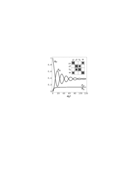
Figure 4: Dynamics of the occupation probabilities for the states $\left|\uparrow\uparrow\right\rangle$, $\left|\uparrow\downarrow\right\rangle$, $\left|\downarrow\uparrow\right\rangle$, and $\left|\downarrow\downarrow\right\rangle$. The parameters are the same as in Figure 2. The inset shows the structure of the reduced density matrix (the nonshaded entries are all zero).

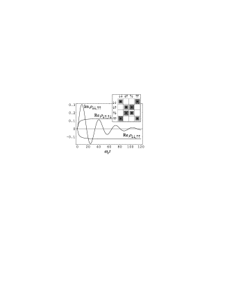
Figure 5: Dynamics of the inverse-diagonal matrix elements for the same system as in Figure 4. Note that ${\rm Im}\,\rho_{\downarrow\uparrow,\uparrow\downarrow}=0$.

V Ohmic and Super-Ohmic Bath Models in General Dimension

Let us generalize the results of the previous sections obtained primarily for the Ohmic bath model and 1D geometry. In Section II, we considered the 1D case with Ohmic dissipation with the Markovian approach. In the general case, let us consider the Markovain model and, again, assume that $\Delta/\omega_{c}$ is small. We will also assume that the absolute square of the $m$th component of the spin-boson coupling, when multiplied by the density of states, can be modelled by $\alpha_{n_{m}}^{m}{}\omega^{n_{m}}\exp(-\omega/\omega_{c})$; see Eq.(2.12). The integration in Eq.(2.8) can then be carried out in closed form for any $n_{m}=1,2,\ldots\,\,$. The induced interaction (2.17) is thus generalized to

$$H_{\textrm{int}}= - \!\!\!\sum\limits_{m=x,y,z}{\alpha_{n_{m}}^{m}\omega_{c}^{n_{m}}\sigma_{m}^{1}\sigma_{m}^{2}}$$

$$\times \frac{{2\Gamma(n_{m})\textrm{Re}\left({1+i\omega_{c}\left|{\mathbf{d}}\right|/c_{s}}\right)^{n_{m}}}}{{\left[{1+\left({\omega_{c}\left|{\mathbf{d}}\right|/c_{s}}\right)^{2}}\right]^{n_{m}}}}.$$

With the appropriate choice of parameters, the result for the induced interaction, but not for the noise, coincides with the expression for $H_{\textrm{int}}$ obtained within the short-time model. From Eq.(V) one can infer that the effective interaction has the large-distance asymptotic behavior $\left|{\mathbf{d}}\right|^{-n_{m}}$, for even $n_{m}$, and $\left|{\mathbf{d}}\right|^{-n_{m}-1}$, for odd $n_{m}$.

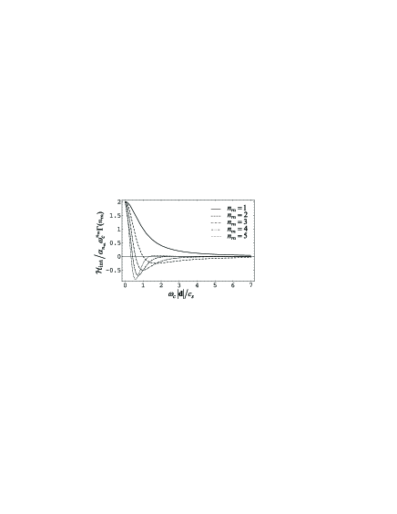
Figure 6: The magnitude of the induced exchange interaction Hamiltonian for the Ohmic $n_{m}=1$ and super-Ohmic $n_{m}=2,3,4,5$ baths.

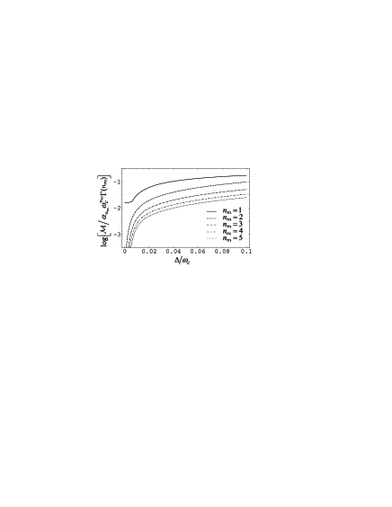
Figure 7: The magnitude of the noise for the Ohmic $n_{m}=1$ and super-Ohmic $n_{m}=2,3,4,5$ baths, for $2k_{\textrm{B}}T/\omega_{c}=0.01$.

Let us now consider the noise terms. The amplitudes (2.9, 2.10), entering the decoherence superoperator, depend on $n_{m}$ only via the prefactor $(\Delta/\omega_{c})^{n_{m}}$. The remaining amplitude (II) has to be calculated numerically. The spin-spin separation up to which the “coherent” effects of the induced interaction can be observed in the time-dependent dynamics, is defined by comparing the magnitudes of the interaction and noise amplitudes. It transpires that the comparison of the amplitude in Eq.(2.17) vs Eq.(2.16) for $n_{m}=1$, also suffices for an approximate estimate for the super-Ohmic case, as long as $\eta^{m}_{s}(\mathbf{d})$ does not dominate in ${\hat{M}}$. In Figure 6, we plot the amplitudes of Eq.(V), i.e., ${\cal H}_{\textrm{int}}\equiv Tr(H_{\textrm{int}}\sigma^{1}_{m}\sigma^{2}_{m})/4$, for different values of $n_{m}$. Figure 7 shows the magnitude of the noise super-operator. Figures 6 and 7 suggest that the noise amplitudes can be made sufficiently small with respect to the induced interaction, at small values of $\Delta/\omega_{c}$, for any $n_{m}$. We note that for quantum computing applications one usually assumes the regime $k_{B}T\ll\Delta\ll\omega_{c}$. The temperature dependence in Fig. 7 becomes insignificant for $k_{B}T/\Delta\ll 1$, which is approximately to the right of $\Delta/\omega_{c}\sim 0.01$. To the left of $\Delta/\omega_{c}\sim 0.01$, by reducing the temperature one can further reduce the values of the noise amplitudes even for small $\Delta$.

In higher dimensions the structure of $g_{{\mathbf{k}},\mathbf{\xi}}^{m}$ in the k-space becomes important. Provided $\omega_{{\mathbf{k}},\mathbf{\xi}}$ is nearly isotropic, the integrals entering Eqs.(2.8)-(II) will include (in 3D) a factor $\int_{0}^{2\pi}{d\varphi}\int_{0}^{\pi}{d\theta\sin\theta}\left|{g_{k\theta\varphi,\mathbf{\xi}}^{m}}\right|^{2}\cos\left({k\left|{\mathbf{d}}\right|\cos\theta}\right)$, which can be written as $[f^{m}_{1}(\omega,k|\mathbf{d}|)-f^{m}_{2}(\omega,k|\mathbf{d}|)\partial/\partial|\mathbf{d}|]\cos(k|\mathbf{d}|)$, e.g., Eqs.(B, B) in Appendix B. When the dependence of $f^{m}_{1},f^{m}_{2}$ on $k|\mathbf{d}|$ is negligible, the interaction is simply $H_{\textrm{int}}\rightarrow H_{\textrm{int}}|_{\{n_{m}\}\rightarrow a}-(\partial/\partial|\mathbf{d}|)H_{\textrm{int}}|_{\{n_{m}\}\rightarrow b}$, where $a$ and $b$ are sets of three integers representing the $\omega$-dependence of $f_{1}^{m}(\omega,k|\mathbf{d}|)$ and $f_{2}^{m}(\omega,k|\mathbf{d}|)$. Otherwise, a more complicated dependence on $|\mathbf{d}|$ is expected. The noise superoperator can be treated similarly. As a result one can see that the form of the interaction depends more on the structure of $g_{{\mathbf{k}},\mathbf{\xi}}^{m}$ than on the dimensionality via the phonon density of states. However, reduced dimensionality in the $\mathbf{k}$-space might allow for better control over the magnitude of the interaction by external potentials that modify the spin-orbit coupling.

VI Phonon Induced Coherent Spin-Spin Interaction vs Noise for P-donor electrons in Si and Ge

As a specific example, let us consider a model of two localized impurity-electron spins of phosphorus donors in a Si-Ge type semiconductor, coupled to acoustic phonon modes by spin-orbit interaction. In what follows, we first obtain the coupling constants $g^{m}_{\mathbf{k},\xi}$, entering Eq.(1.3), which define the interaction and noise amplitudes. A brief discussion is then offered on the possibility of having an Ohmic bath model realized in 1D channels. The rest of the present section is devoted to calculations of the induced interaction and noise in 3D bulk material. A comparison with the dipole-dipole spin interaction is given.

Averaging the spin orbit Hamiltonian over the localized electron’s wave function, one obtains the spin-orbit coupling in the presence of magnetic field $\mathbf{H}=(H_{x},H_{y},H_{z})$ in the form

$$H_{\textrm{SO}}=\mu_{\textrm{B}}\!\!\sum\limits_{m,l\,=\,x,y,z}\!\!{\sigma_{m}g_{ml}H_{l}},$$ (6.1)

where $\mu_{\textrm{B}}$ is the Bohr magneton. Here the tensor $g_{ml}$ is sensitive to lattice deformations. It was shownRoth that for the donor state which has tetrahedral symmetry, the Hamiltonian (6.1) yields the spin-deformation interaction of the form

$$H = {\rm A}\mu_{\textrm{B}}\left[{\bar{\varepsilon}_{xx}\sigma_{x}H_{x}+\bar{\varepsilon}_{yy}\sigma_{y}H_{y}+\bar{\varepsilon}_{zz}\sigma_{z}H_{z}+{\bar{\Delta}}(\mathbf{\sigma}\cdot\mathbf{H}})/3\right]$$ (6.2)

$$+ {\rm B}\mu_{\textrm{B}}\left[{\bar{\varepsilon}_{xy}\left({\sigma_{x}H_{y}+\sigma_{y}H_{x}}\right)+{\text{c}}{\text{.p}}{\text{.}}}\right].$$

Here c.p. denotes cyclic permutations and $\bar{\Delta}$ is the effective dilatation. The tensor $\bar{\varepsilon}_{ij}$ already includes averaging of the strain with the gradient of the potential over the donor ground state wave function.

As before, let us assume that the separation d, as well as the magnetic field, are directed along the $z$-axis, for an illustrative calculation. Then the spin-deformation interaction Hamiltonian simplifies to

$$H={\rm A}\mu_{\textrm{B}}\bar{\varepsilon}_{zz}\sigma_{z}H_{z}+{\rm B}\mu_{\textrm{B}}\left({\bar{\varepsilon}_{yz}\sigma_{y}H_{z}+\bar{\varepsilon}_{zx}\sigma_{x}H_{z}}\right).$$ (6.3)

In terms of the quantized phonon field, we haveMahan ; MKGB

$$\bar{\varepsilon}_{ij}=\sum\limits_{{\mathbf{k}},{\mathbf{\xi}}}{f({\mathbf{k}})\sqrt{\frac{\hbar}{{8\rho V\omega_{{\mathbf{k}},{\mathbf{\xi}}}}}}\left({\xi_{{\mathbf{k}},i}k_{j}+\xi_{{\mathbf{k}},j}k_{i}}\right)\left({a_{{\mathbf{k}},{\mathbf{\xi}}}^{\dagger}+a_{{\mathbf{k}},{\mathbf{\xi}}}}\right)},$$ (6.4)

where in the spherical donor ground state approximationHasegawa ; MKGB

$$f({\mathbf{k}})=\frac{1}{{\left({1+a_{\textrm{B}}^{2}k^{2}}\right)^{2}}}.$$ (6.5)

Here $a_{\textrm{B}}$ is half the effective Bohr radius of the donor ground state wave function. In an actual Si or Ge crystal, donor states are more complicated and include corrections due to the symmetry of the crystal matrix including the fast Bloch-function oscillations. However, the wave function of the donor electrons in our case is spread over several atomic dimensions (see below). Therefore, it suffices to consider “envelope” quantities. Thus, the spin-phonon Hamiltonian (1.2, 1.3) coupling constants will be taken in the form

$$g_{{\mathbf{k}},{\mathbf{\xi}}}^{m}=\frac{D_{m}}{{\left({1+a_{\textrm{B}}^{2}k^{2}}\right)^{2}}}\sqrt{\frac{\hbar}{{8\rho V\omega_{{\mathbf{k}},{\mathbf{\xi}}}}}}\left({\xi_{{\mathbf{k}},z}k_{m}+\xi_{{\mathbf{k}},m}k_{z}}\right),$$ (6.6)

where $D_{x}=D_{y}={\rm B}\mu_{\textrm{B}}H_{z}$ and $D_{z}={\rm A}\mu_{\textrm{B}}H_{z}$.

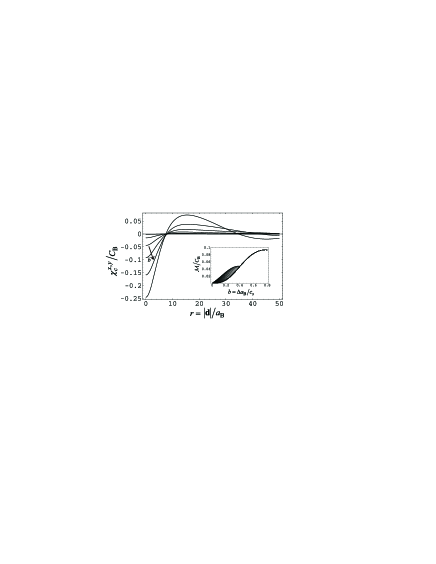
Figure 8: The magnitude of the induced spin-spin interaction for a 3D Si-Ge type structure: The dominant interaction amplitude, which is the same for the $x$ and $y$ spin components, is shown. The arrow indicates increasing $b$ values for the curves shown, with $b=0.03$, $0.09$, $0.15$, $0.21$, $0.27$, $0.33$. The inset estimates the level of the noise (for $2k_{B}Ta_{B}/c_{s}=0.01$): The bottom curve is $\eta_{c}^{m}(0)$, with $m=x,y$. For $b\lesssim 0.4$, the amplitude $\eta_{s}^{m}(\mathbf{d})$ can be comparable, and its values, calculated numerically for $0\leq r\leq 50$, are shown as long as they exceed $\eta_{c}^{m}(0)$, with the top curve corresponding to the maximum value, at $r=0$.

Let us first consider a 1D channel geometry along the $z$ direction. This will give an example of an Ohmic bath model discussed towards the end of Section II. In 1D channel the boundariesPBS can approximately quantize the spectrum of phonons along $x$ and $y$, depleting the density of states except at certain resonant values. Therefore, the low-frequency effects, including the induced coupling and quantum noise, will become effectively onedimensional, especially if the effective gap due to the confinement is of the order of $\omega_{c}$. As mentioned earlier, this frequency cutoff comes from Eq.(6.5), namely, it is due to the bound electron wave function localization. A channel of width comparable to $\sim a_{\textrm{B}}$ will be required. This, however, may be difficult to achieve in bulk Si or Ge with the present-day technology. Other systems may offer more immediately available 1D geometries for testing similar theories, for instance, carbon nanotubes, chains of ionized atoms suspended in ion traps,Porras ; Marquet ; Leibfried etc. In our case, the longitudinal acoustic (LA, $||$) phonons of the one-dimensional spectrum will account for the $g_{\mathbf{k},\parallel}^{z}$ component of the coupling, whereas the transverse acoustic (TA, $\perp$) phonons will affect only the $x$ and $y$ spin projections.

One can show that the contributions of the crossproducts of coupling constants, $g_{\mathbf{k},\mathbf{\xi}}^{m}(g_{\mathbf{k},\mathbf{\xi}}^{m^{\prime}})^{*}$ with $m\neq m^{\prime}$, to quantities of interest vanish. The diagonal combinations are

$$|g_{k_{z}}^{z}|^{2} = \frac{\textrm{A}^{2}\mu_{\textrm{B}}^{2}H_{z}^{2}}{{4\rho V\omega_{k_{z},\parallel}}}\frac{{k_{z}^{2}}}{{\left({1+a_{\textrm{B}}^{2}k_{z}^{2}}\right)^{4}}},$$ (6.7)

$$|g_{k_{z}}^{x}|^{2} = |g_{k_{z}}^{y}|^{2}=\frac{\textrm{B}^{2}\mu_{\textrm{B}}^{2}H_{z}^{2}}{{4\rho V\omega_{k_{z},\bot}}}\frac{{k_{z}^{2}}}{{\left({1+a_{B}^{2}k_{z}^{2}}\right)^{4}}}.$$

With our usual assumption for the low-frequency dispersion relations $\omega_{k_{z},\parallel}\approx c_{\parallel}k_{z}$ and $\omega_{k_{z},\perp}\approx c_{\perp}k_{z}$, the expressions (6.7) lead to the Ohmic bath model discussed at the end of Section II. The shape of the frequency cutoff resulting from Eq.(6.7) is not exponential. However, to estimate the magnitude of the interaction and noise one can utilize the results obtained earlier for the 1D Ohmic bath model with exponential cutoff. The coupling constants in Eqs.(2.17) and (2.16) should, then, be taken as

$$\alpha_{1}^{z} = \frac{\textrm{A}^{2}\mu_{\textrm{B}}^{2}H_{z}^{2}}{8\pi\rho Sc^{3}_{\parallel}},$$ (6.8)

$$\alpha_{1}^{x} = \alpha_{1}^{y}=\frac{\textrm{B}^{2}\mu_{\textrm{B}}^{2}H_{z}^{2}}{8\pi\rho Sc^{3}_{\bot}},$$

where $S$ is a cross section of the channel, and the cutoff is $\omega_{c}\rightarrow c_{\parallel}/a_{\textrm{B}}$ for the $z$ component, and $\omega_{c}\rightarrow c_{\perp}/a_{\textrm{B}}$ for the $x$ and $y$ components. Considering Si as an example, we arrive at an approximately adiabatic Hamiltonian ($\alpha_{1}^{z}\gg\alpha_{1}^{x,y}$) with Ohmic-type coupling. The dynamics of the concurrence, then, is qualitatively similar to the one shown on Fig. 2, with the peak entanglement $\sim 0.4$ as well. The coupling constant $\alpha_{1}^{z}$, however, is significantly smaller due to the weakness of the spin-orbit coupling of P-impurity electrons in Si, which results in low magnitude of the induced interaction (and the noise due to the same environment), and slightly modifies the shape of the concurrence.

In the 3D geometry, let us consider for simplicity only the LA phonon branch, ${\mathbf{\xi}}\to{\mathbf{k}}/\left|{\mathbf{k}}\right|$, and assume an isotropic dispersion $\omega_{\mathbf{k},\mathbf{\xi}}=c_{s}\left|\mathbf{k}\right|$. The expression for the coupling constants is then

$$g_{{\mathbf{k}},{\mathbf{\xi}}}^{m}=D_{m}\frac{{k_{z}k_{m}}}{{\left({1+a_{\textrm{B}}^{2}k^{2}}\right)^{2}}}\sqrt{\frac{\hbar}{{2\rho Vc_{s}k^{3}}}}.$$ (6.9)

The cross terms, with $m\neq n$, of the correlation functions $Tr_{B}\left[X_{m}^{j}X_{n}^{i}(t)\rho_{B}\right]$, see Eq.(A.3) in Appendix A, depend on the combination $g_{\mathbf{k},\mathbf{\xi}}^{m}(g_{\mathbf{k},\mathbf{\xi}}^{n})^{*}$, which is always an odd function of one of the projections of the wave vector. The nondiagonal terms thus vanish, as mentioned in Appendix A.

Integrating Eqs.(2.8) and (2.9) with Eq.(6.9), see Appendix B, one can demonstrate that decoherence is dominated by the individual noise terms for each spin, with the typical amplitude

$$\eta_{c}^{x,y}(0)=C_{\textrm{B}}\frac{{2\pi^{2}}}{{15}}\frac{b^{3}}{\left({1+b^{2}}\right)^{4}}\coth\frac{\Delta}{2k_{\textrm{B}}T},$$ (6.10)

where $b=\Delta a_{B}/c_{s}$ and $C_{\textrm{B}}={\rm B}^{2}\mu_{B}^{2}H_{z}^{2}/\left({16\pi^{3}\rho\hbar a_{B}^{3}c_{s}^{2}}\right)$. The interaction amplitude $\chi_{c}^{m}({\mathbf{d}})$ and, therefore, the induced spin-spin interaction, has inverse-square power-law asymptotic form for the $x$ and $y$ spin components, with a superimposed oscillation, and inverse-fifth-power-law decay for the $z$ spin components

$$H_{\textrm{int}} = \sum\nolimits_{m}{2\chi_{c}^{m}({\mathbf{d}})\sigma_{m}^{1}\sigma_{m}^{2}}$$ (6.11)

$$\xrightarrow{{r\gg 1}} - 4\pi^{2}C_{\textrm{B}}\frac{{2b}}{{\left({1+b^{2}}\right)^{4}}}\frac{{\sin br}}{{r^{2}}}\left({\sigma_{x}^{1}\sigma_{x}^{2}+\sigma_{y}^{1}\sigma_{y}^{2}}\right)$$

$$+ 384\pi^{2}C_{\textrm{A}}\frac{2}{{r^{5}}}\sigma_{z}^{1}\sigma_{z}^{2}.$$

Here $r=|\mathbf{d}|/a_{\textrm{B}}$ and $C_{\textrm{A}}=\textrm{A}^{2}C_{\textrm{B}}/\textrm{B}^{2}$. At small distances the interaction is regular and the amplitudes converge to constant values, see Figure 8. The complete expressions for $\chi_{c}^{m}(\mathbf{d})$ and $\eta_{c}^{m}(\mathbf{d})$ are given in Appendix B.

In Figure 8, we plot the amplitudes of the induced spin-spin interaction (6.11, B.4, B.7) and noise for different values of the spin-spin separation and $b$, for electron impurity spins in 3D Si-Ge type structures. The value of $b$ can be controlled via the applied magnetic field, $b=\mu_{\textrm{B}}H_{z}g^{*}a_{\textrm{B}}/c_{s}$. The temperature dependence of the noise is insignificant provided $2k_{B}T/\Delta\ll 1$.

A typical valueHasegawa ; Roth ; MKGB of the effective Bohr radius in Si for the P-donor-electron ground state wave function is $2a_{\textrm{B}}=2.0\,$nm. The crystal lattice density is $\rho=2.3\times 10^{3}\,$kg/m³, and the g-factor $g^{*}=1.98$. For an order-of-magnitude estimate, we take a typical value of the phonon group velocity, $c_{s}=0.93\times 10^{4}\,$m/s. The spin-orbit coupling constants in Si areHasegawa ; Roth ; MKGB $\textrm{A}^{2}\approx 10^{2}$ and $\textrm{B}^{2}\approx 10^{-1}$. The resulting interaction constants in Eqs.(6.10, 6.11) are $C_{\textrm{B}}=7.8\,$s^-1 and $C_{\textrm{A}}=10^{3}C_{\textrm{B}}$. In the Ge lattice, the spin-orbit coupling is dominated by the non-diagonal terms,Hasegawa ; Roth ; MKGB $\textrm{A}^{2}\approx 0$ and $\textrm{B}^{2}\approx 10^{6}$. The other parameters are $2a_{\textrm{B}}=4.0\,$nm, $\rho=5.3\times 10^{3}\,$kg/m³, $c_{s}=5.37\times 10^{3}\,$m/s, and $g^{*}=1.56$. This results in a much stronger transverse component interaction, $C_{\textrm{B}}=1.3\times{}10^{7}\,$s^-1 and $C_{\textrm{A}}\approx 0$. In both cases the magnetic field was taken $H_{z}=3\times 10^{4}\,$G. In the above estimations, one could use various experimentally suggested values for the parameters, such as, for instance, $a_{B}$. This will not affect the results significantly.

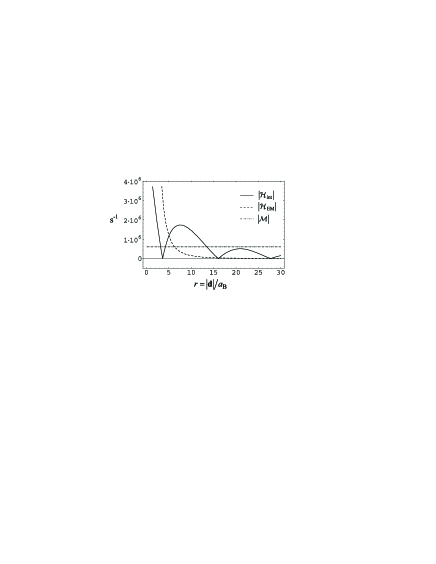
Figure 9: The magnitudes, measured in units of s^-1, of the induced spin-spin interaction, the EM coupling strength, and the level of noise for P-impurity electron spins in Ge. Here $H_{z}=3\times 10^{4}\,$G, and low temperature, $2k_{\textrm{B}}T/\Delta\ll 1$, was assumed.

As mentioned is Section II, the obtained interaction (6.11) is always accompanied by noise coming from the same source, as well as possibly by other, direct interactions of the spins. When the electron wave functions overlap is negligible, the dominant direct interaction will be the dipole-dipole one

$$H_{\textrm{EM}}(\mathbf{d})=\frac{\mu_{0}\mu_{\textrm{B}}^{2}}{4\pi}\frac{\sigma_{x}^{1}\sigma_{x}^{2}+\sigma_{y}^{1}\sigma_{y}^{2}-2\sigma_{z}^{1}\sigma_{z}^{2}}{|\mathbf{d}|^{3}}.$$ (6.12)

The comparison of the two interactions and noise is shown in Figure 9. We plot the magnitude of the effective induced interaction (6.11, B.4, B.7), the electromagnetic interaction (6.12), measured by ${\cal H}_{\textrm{EM}}\equiv{\mu_{0}\mu_{\textrm{B}}^{2}}/{4\pi|\mathbf{d}|^{3}}$, and a measure of the level of noise, for P-donor electron spins in Ge. It transpires that the induced interaction can be considerable as compared to the electromagnetic spin-spin coupling. However the overall coherence-to-noise ratio is quite poor for Ge. In Si, the level of noise is lower as compared to the induced interaction. However, the overall amplitude of the induced terms compares less favorably with the electromagnetic coupling.

In conclusion, we have studied the induced indirect exchange interaction due to a bosonic bath which also introduces quantum noise. We demonstrated that it can create substantial two-spin entanglement. For an appropriate choice of the system parameters, specifically, the spin-spin separation, for low enough temperatures this entanglement can be maintained and the system can evolve approximately coherently for many cycles of its internal dynamics. For larger times, the quantum noise effects will eventually dominate and the entanglement will be erased.

Estimates for P-impurity electron spins in Si and Ge structures have demonstrated that the induced interaction can be comparable to the dipole-dipole spin interaction. One can also infer that this phonon-mediated interaction in the bulk (3D) Ge is not very effective to be used for quantum computing purposes, i.e., to entangle qubits. This is due to poor coherence to noise ratio. Therefore, the use of Si may be favored, despite the fact that it has weaker spin-phonon coupling. Indeed, the noise amplitudes for Si are significantly smaller then the induced exchange interaction, where the latter is dominated by the adiabatic term. The situation is expected to be further improved for systems with reduced dimensionality for phonon propagation.

Appendix A Derivation Steps for the Induced Interaction and Noise

An important assumption required for the validity of the Markovian approach concerns the time scale of the decay of the bath correlations introduced in Eqs.(A.2) and (A.3) below. By constantly resetting the bath to thermal, one implies that this time scale is significantly shorter than the dynamical system time scales of interest. The Markovian treatment, considered here, is, therefore, valid at all but very short times. The short-time dynamics, for the time scales down to order $1/\omega_{c}$, requires a different approach.Privman ; Tolkunov2 ; Solenov Note that one usually assumes that $\omega_{c}\gg\Delta$.

Here we review some of the steps that lead from the Markovian equation for the density matrix (II), to the expressions for the induced interaction and quantum noise. Substituting Eqs.(1.2) and (1.3) in Eq.(II), one can represent the integrand, $Tr_{B}[H_{SB},[H_{SB}(t^{\prime}-t),\rho_{B}\rho_{S}(t)]]\rho_{S}(t)$, as a summation over $i,j,m,n$, of the following expression:

$$\hphantom{+}Tr_{B}\left({X^{j}_{m}X^{i}_{n}(t^{\prime}-t)\rho_{B}}\right)\sigma^{j}_{m}\sigma^{i}_{n}(t^{\prime}-t)\rho_{S}(t)$$

$$-Tr_{B}\left({X^{j}_{m}\rho_{B}X^{i}_{n}(t^{\prime}-t)}\right)\sigma^{j}_{m}\rho_{S}(t)\sigma^{i}_{n}(t^{\prime}-t)$$ (A.1)

$$-Tr_{B}\left({X^{i}_{n}(t^{\prime}-t)\rho_{B}X^{j}_{m}}\right)\sigma^{i}_{n}(t^{\prime}-t)\rho_{S}(t)\sigma^{j}_{m}$$

$$+Tr_{B}\left({\rho_{B}X^{i}_{n}(t^{\prime}-t)X^{j}_{m}}\right)\rho_{S}(t)\sigma^{i}_{n}(t^{\prime}-t)\sigma^{j}_{m}.$$

Here $\sigma_{n}^{i}(t)=e^{iH_{S}t}\sigma_{n}^{i}{}e^{-iH_{S}t}$. All the terms in Eq.(A.1) involve the correlation functions

$$C_{mn}\left({(1-\delta_{ij}){\mathbf{d}},t}\right)=Tr_{B}X_{m}^{j}X_{n}^{i}(t)\rho_{B},$$ (A.2)

where $X_{n}^{i}(t)=e^{iH_{B}t}X_{n}^{i}{}e^{-iH_{B}t}$. The explicit expression for these functions can then be obtained from Eqs.(1.3) and (A.2),

$$C_{mn}({\mathbf{d}},t)=\frac{V}{{\left({2\pi}\right)^{3}}}\sum\limits_{\mathbf{\xi}}\!{\int\limits_{-\infty}^{\infty}\!\!{d{\mathbf{k}}}}\left|{g_{{\mathbf{k}},\mathbf{\xi}}^{m}g_{{\mathbf{k}},\mathbf{\xi}}^{n}}\right|\Big{[}{i\sin\omega_{{\mathbf{k}},\mathbf{\xi}}t}\phantom{\frac{a}{b}}$$ (A.3)

$$+\,{\coth\frac{{\omega_{{\mathbf{k}},\mathbf{\xi}}}}{{2k_{\textrm{B}}T}}\cos\omega_{{\mathbf{k}},\mathbf{\xi}}t}\Big{]}\cos\left({{\mathbf{k}}\cdot{\mathbf{d}}+\phi_{{\mathbf{k}},\mathbf{\xi}}^{n}-\phi_{{\mathbf{k}},\mathbf{\xi}}^{m}}\right),$$

where $\phi_{\mathbf{k},\xi}^{n}$ is a possible phase of the coupling constants $g_{\mathbf{k},\xi}^{n}$, which is not present in most cases. The coupling constants are examined in detail in Sections V and VI, and explicit model expressions are given. Presently, we only comment that in many cases the resulting matrix of the correlation functions $C_{mn}({\mathbf{d}},t)$ is diagonal, which simplifies calculations, as illustrated in Section VI.

The summation of Eq.(A.1) over $i,j,m,n$ is further simplified by noting that $C_{mn}(\mathbf{d},t)=C^{*}_{mn}(\mathbf{d},-t)$, and writing $\sigma_{n}^{i}(t)$ explicitly as $\sigma_{z}^{i}$ for $n=z$, and $\sigma_{n}^{i}\cos\Delta t+\frac{1}{2}[\sigma_{z}^{i},\sigma_{n}^{i}]\sin\Delta t$ for $n\neq z$. For a diagonal $C_{m,n}$, we then get the amplitude expressions

$$\int\limits^{0}_{-\infty}dt^{\prime}\textrm{Im}C_{mm}(\mathbf{d},t^{\prime})\cos(\Delta t^{\prime})=\chi_{c}^{m}(\mathbf{d}),$$ (A.4)

$$\int\limits^{0}_{-\infty}dt^{\prime}\textrm{Im}C_{mm}(\mathbf{d},t^{\prime})\sin(\Delta t^{\prime})=\chi_{s}^{m}(\mathbf{d}),$$ (A.5)

$$\int\limits^{0}_{-\infty}dt^{\prime}\textrm{Re}C_{mm}(\mathbf{d},t^{\prime})\cos(\Delta t^{\prime})=\eta_{c}^{m}(\mathbf{d}),$$ (A.6)

$$\int\limits^{0}_{-\infty}dt^{\prime}\textrm{Re}C_{mm}(\mathbf{d},t^{\prime})\sin(\Delta t^{\prime})=\eta_{s}^{m}(\mathbf{d}).$$ (A.7)

This finally leads to Eqs.(LABEL:eq:S2:H-eff) and (2.5).

Appendix B Interaction and Noise Amplitudes for Si-Ge type Spin-Orbit Coupling

In Eqs.(2.8) and (2.9), with Eq.(6.9), there is a common angular part

$$I_{m}(kd)=\int\limits_{0}^{2\pi}d\varphi\int\limits_{0}^{\pi}\sin\theta d\theta\frac{k_{z}^{2}k_{m}^{2}}{k^{4}}cos(kd\cos\theta),$$ (B.1)

which gives

$$I_{x,y}(kd) = 4\pi\operatorname{Re}\frac{{12-k^{2}d^{2}}}{{k^{4}d^{4}}}e^{ikd}$$

$$- 4\pi\operatorname{Re}i\frac{{5k^{2}d^{2}-12}}{{k^{5}d^{5}}}e^{ikd}$$

and

$$I_{z}(kd) = 16\pi\operatorname{Re}\frac{{k^{2}d^{2}-6}}{{k^{4}d^{4}}}e^{ikd}$$

$$- 4\pi\operatorname{Re}i\frac{{k^{4}d^{4}-12k^{2}d^{2}+24}}{{k^{5}d^{5}}}e^{ikd}.$$

Here $d\equiv|\mathbf{d}|$. The remaining integral in Eq.(2.8),

$$\chi_{c}^{x,y}({\mathbf{d}})=-\frac{D_{m}^{2}}{2\rho{\left({2\pi}\right)^{3}}c_{s}}{\int\limits_{-\infty}^{\infty}}\frac{I_{x,y}(kd)}{\left({1+a_{\textrm{B}}^{2}k^{2}}\right)^{4}}\frac{{c_{s}k^{4}dk}}{{c_{s}^{2}k^{2}-\Delta^{2}}},$$ (B.4)

can be evaluated along a contour in the upper complex plane. The integration contour includes two simple poles, at $k=\pm\Delta/c_{s}$, which have to be taken with weight $1/2$ due to principal value integration. Also included is the pole at $k=i/a_{\textrm{B}}$, of order four, and a simple pole at $k=0$ (with weight $1/2$). The latter pole is for the second term in Eq.(B) only.

The pole at $k=i/a_{\textrm{B}}$ yields exponentially decaying terms $\sim\exp(-d/a_{\textrm{B}})$. At large $d$, the asymptotic behavior is controlled by the poles at $k=\pm\Delta/c_{s}$,

$$\chi_{c}^{x,y}({\mathbf{d}})\xrightarrow{{r\gg 1}}-4\pi^{2}C_{\textrm{B}}\frac{{2b}}{{\left({1+b^{2}}\right)^{4}}}\frac{{\sin br}}{{r^{2}}},$$ (B.5)

where $b=\Delta a_{B}/c_{s}$ and $r=|\mathbf{d}|/a_{\textrm{B}}$. The complete expression can be easily obtained from Eq.(B.4). One can also note that at $d\rightarrow 0$, Eq.(B.4) is

$$\chi_{c}^{x,y}({\mathbf{d}})=-4\pi^{2}C_{B}\frac{{1+9b^{2}-9b^{4}+b^{6}}}{{240\left({1+b^{2}}\right)^{4}}}+O(r^{2}).$$ (B.6)

Along the same contour, the $z$ component of Eq.(2.8),

$$\chi_{c}^{z}({\mathbf{d}})=-\frac{D_{m}^{2}}{2\rho{\left({2\pi}\right)^{3}}c_{s}^{2}}{\int\limits_{-\infty}^{\infty}}\frac{I_{x,y}(kd)k^{2}dk}{\left({1+a_{\textrm{B}}^{2}k^{2}}\right)^{4}}$$ (B.7)

has only two poles, at $k=0$ [order 2 for the first term, and also of order 1 or 3 for the second term in $I_{z}(kd)$], and at $k=i/a_{\textrm{B}}$ (of order 4). The pole at $k=0$ is to be taken with weight $1/2$ and gives the $1/r^{5}$ asymptotic,

$$\chi_{c}^{z}({\mathbf{d}})\xrightarrow{{r\gg 1}}384\pi^{2}C_{\textrm{A}}\frac{1}{{r^{5}}},$$ (B.8)

while for $r\rightarrow 0$ one obtains

$$\chi_{c}^{z}({\mathbf{d}})=-C_{A}\frac{{\pi^{2}}}{{20}}+O(r^{2}).$$ (B.9)

Substituting Eqs.(B.5) and (B.8) in $H_{\textrm{int}}$, i.e., in the second term in Eq.(LABEL:eq:S2:H-eff), one obtains Eq.(6.11).

By using Eqs.(B.1) and (B), for Eq.(2.9) we obtain

$$\eta_{c}^{x,y}({\mathbf{d}})=\frac{\pi}{2}C_{B}\frac{{b^{3}}}{{\left({1+b^{2}}\right)^{4}}}I_{x,y}(rb)\coth\frac{\Delta}{{2k_{\textrm{B}}T}}.$$ (B.10)

The decoherence processes are dominated by the local noise terms, e.g., $\eta_{c}^{x,y}(0)$. Noting that $I_{x,y}(0)=\frac{4\pi}{15}$, one obtains (6.10). One also finds that $\eta_{c}^{z}(\mathbf{d})=0$. For low temperatures, $\frac{\Delta}{2k_{\textrm{B}}T}\gg 1$, one has $\coth\frac{\Delta}{2k_{\textrm{B}}T}\approx 1$ and, therefore, $\chi_{s}^{m}(\mathbf{d})\approx\eta_{c}^{m}(\mathbf{d})$, see Eqs.(2.10) and (2.9). Note that the expressions involving $\chi_{s}^{m}(\mathbf{d})$ can be neglected in (LABEL:eq:S2:H-eff), since the corrections they introduce to the induced interaction have the same magnitude as the noise amplitudes. The function $\eta_{s}^{m}(\mathbf{d})$ is often comparable to $\eta_{c}^{m}(\mathbf{d})$ for Eq.(6.9) with the parameters used in Section VI. This amplitude is calculated numerically in Figure 8.

References

(1) G. D. Mahan, Many-Particle Physics (Kluwer Academic, New York, 2000).
(2) M. Xiao, I. Martin, E. Yablonovitch, and H. W. Jiang, Nature 430, 435
(2004).
(3) M. R. Sakr, H. W. Jiang, E. Yablonovitch, and E. T. Croke,
Appl. Phys. Lett. 87, 223104 (2005).
(4) N. J. Craig, J. M. Taylor, E. A. Lester, C. M. Marcus, M. P. Hanson, and A. C. Gossard, Science 304, 565 (2004).
(5) J. M. Elzerman, R. Hanson, L. H. Willems van Beveren, B. Witkamp, L. M. K. Vandersypen, and L. P. Kouwenhoven, Nature 430, 431 (2004).
(6) F. H. L. Koppens, C. Buizert, K. J. Tielrooij, I. T. Vink, K. C.
Nowack, T. Meunier, L. P. Kouwenhoven, and L. M. K. Vandersypen,
Nature 442, 766 (2006).
(7) J. R. Petta, A. C. Johnson, J. M. Taylor, E. A. Laird, A. Yacoby, M. D. Lukin, C. M. Marcus, M. P. Hanson, and A. C. Gossard, Science 309, 2180 (2005).
(8) I. Martin, D. Mozyrsky, and H. W. Jiang, Phys. Rev. Lett. 90,
018301 (2003).
(9) E. Prati, M. Fanciulli, A. Kovalev,
J. D. Caldwell, C. R. Bowers, F. Capotondi, G. Biasiol, and L.
Sorba, IEEE Trans. Nanotechnol. 4, 100 (2005).
(10) D. Solenov, D. Tolkunov, and V. Privman, Phys. Lett. A 359, 81 (2006).
(11) D. Braun, Phys. Rev. Lett. 89, 277901 (2002).
(12) T. Yu and J. H. Eberly, Phys. Rev. B 68, 165322 (2003).
(13) T. Yu and J. H. Eberly, Phys. Rev. Lett. 93, 140404 (2004).
(14) D. Tolkunov, V. Privman, and P. K. Aravind, Phys. Rev. A 71, 060308 (2005).
(15) M.A. Ruderman and C. Kittel, Phys. Rev. 96, 99 (1954); T. Kasuya, Prog. Theor. Phys. 16, 45 (1956);
K. Yosida, Phys. Rev. 106, 893 (1957).
(16) Yu. A. Bychkov, T. Maniv, and I. D. Vagner, Solid State Comun. 94, 61 (1995).
(17) V. Privman, I. D. Vagner, and G. Kventsel, Phys. Lett. A 239, 141 (1998).
(18) D. Mozyrsky, V. Privman, and I. D. Vagner, Phys. Rev. B 63, 085313 (2001).
(19) D. Mozyrsky, V. Privman, and M. L. Glasser, Phys. Rev. Lett. 86, 5112 (2001).
(20) C. Piermarocchi, P. Chen, L. J. Sham, and D. G. Steel, Phys. Rev. Lett. 89, 167402 (2002).
(21) D. Porras and J. I. Cirac, Phys. Rev. Lett. 92, 207901 (2004).
(22) D. Mozyrsky, A. Dementsov, and V. Privman, Phys. Rev. B 72, 233103 (2005).
(23) Y. Rikitake and H. Imamura, Phys. Rev. B 72, 033308 (2005).
(24) H. Hasegawa, Phys. Rev. 118, 1523 (1960).
(25) L. M. Roth, Phys. Rev. 118, 1534 (1960).
(26) R. Winkler, Spin-Orbit Coupling Effects in Two-Dimentional
Electron and Hole Systems (Springer, New York, 2003).
(27) A. J. Leggett, S. Chakravarty, A. T. Dorsey, M. P. A. Fisher, A.
Garg, and W. Zwerger, Rev. Mod. Phys. 59, 1 (1987).
(28) N. G. van Kampen, Stochastic Processes in Physics and Chemistry (North-Holland, Amsterdam, 2001).
(29) W. H. Louisell, Quantum Statistical Properties of Radiation (Wiley, New York, 1973).
(30) K. Blum, Density Matrix Theory and Applications (Plenum Press, New York, 1996).
(31) V. Privman, Modern Phys. Lett. B 16, 459 (2002).
(32) D. Tolkunov and V. Privman, Phys. Rev. A 69, 062309 (2004).
(33) D. Solenov and V. Privman, Int. J. Modern Phys. B 20, 1476 (2006).
(34) C. Marquet, F. Schmidt-Kaler, and D. F. V. James, Appl. Phys. B 76, 199 (2003).
(35) D. Leibfried, R. Blatt, C. Monroe, and D. Wineland, Rev. Mod. Phys. 75, 281 (2003).
(36) G. M. Palma, K.-A. Suominen, and A. K. Ekert, Proc. R. Soc. London Ser. A 452, 576 (1996).
(37) S. Hill and W. K. Wootters, Phys. Rev. Lett. 78, 5022 (1997).
(38) W. K. Wootters, Phys. Rev. Lett. 80, 2245 (1998).
(39) C. H. Bennett, D. P. DiVincenzo, J. A. Smolin, and W. K. Wootters, Phys. Rev. A 54, 3824 (1996).
(40) V. Vedral, M. B. Plenio, M. A. Rippin, and P. L. Knight, Phys. Rev. Lett. 78, 2275 (1997).
(41) D. Mozyrsky, Sh. Kogan, V. N. Gorshkov, and G. P. Berman, Phys. Rev. B 65, 245213 (2002).
(42) M. Asheghi, Y. K. Leung, S. S. Wong, and K. E. Goodson, Appl. Phys. Lett. 71, 1798 (1997).