Phase transition in liquid crystal elastomer - a Monte Carlo study employing non-Boltzmann sampling

Abstract

We investigate Isotropic - Nematic transition in liquid crystal elastomers employing non-Boltzmann Monte Carlo techniques. We consider a lattice model of a liquid elastomer and a recently proposed Hamiltonian which accounts for homogeneous/inhomogeneous interactions among liquid crystalline units, interaction of local nematics with global strain, and with inhomogeneous fields and stress. We find that when the local director is coupled strongly to the global strain the transition is strongly first order; the transition becomes weakly first order when the coupling becomes weaker. The transition temperature decreases with decrease of coupling strength. Besides, we find that the nematic order scales nonlinearly with global strain especially for strong coupling and at low temperatures.

I Introduction

A liquid crystal elastomer MWEMT is a weakly cross-linked, percolating network of long, rigid, liquid crystalline units. It inherits and combines the properties of both of its components - rubber elasticity of the cross-linked network and nematic and smectic ordering capabilities of the liquid crystalline units. As a result, a liquid crystal elastomer exhibits unusual properties that are of interest from both basic basic1 ; basic2_strain and applied science strain ; artificial_muscles ; tknpjcsr ; ccm ; artemt ; stskr points of views. For example even a small change in temperature (that causes the liquid crystalline units to transform from nematic to isotropic phase) can lead to large and reversible changes in the shape of a liquid crystal elastomer basic2_strain ; strain . It is precisely this property that makes it a competitive candidate material for artificial muscles, see e.g. artificial_muscles ; tknpjcsr . In fact, since liquid crystal elastomers respond sensitively, not only to temperature, but also to other stimuli, like electric fields, magnetic fields, ultra violet radiations, gamma rays etc., they become suitable for construction of actuators, detectors, micro-pumps etc., see e.g. tknpjcsr ; ccm ; artemt ; stskr .

We have carried out Monte Carlo simulation of a lattice model, employing non-Boltzmann sampling techniques. The transition from disordered isotropic phase at high temperatures to ordered nematic phase at low temperatures is known to be weakly first order, in bulk liquid crystalline material, see e.g. SC . Our simulations show that in a liquid crystal elastomer, when the local nematic is coupled strongly to global elastic order the transition is strongly first order; the transition becomes weak when the coupling strength decreases. It is known that the above model exhibits strong discontinuity for $\gamma=1$ sr and a weak discontinuity for $\gamma=0$, see Zhang . Our work interpolates these two limiting cases. More importantly, we find that the nematic order $S$, scales non-linearly with the strain parameter $\lambda$, for strong coupling and at low temperatures. Our Monte Carlo simulations are based on a modified jsm Wang-Landau implementation W_L of entropic sampling techniques BNJL useful for studying complex systems in the neighbourhood of phase transition. In general, entropic sampling BNJL and related techniques W_L enable calculation of the macroscopic properties of a closed system over a wide range and at arbitrarily fine resolution of temperatures - all from a single entropic ensemble that contains microstates of all energies in approximately equal proportions. More importantly these techniques help estimate free energy and entropy, a task which is very difficult, if not impossible, in conventional Metropolis Markov chain Monte Carlo techniques. From the plots of free energy versus order parameter at various temperatures, we can unambiguously determine the nature of the phase transition. The paper is organized as follows. In section II we describe a lattice model of liquid crystal elastomer and the Hamiltonian, proposed by Selinger and Ratna sr . In section III we describe the non-Boltzmann Monte Carlo simulation techniques employed for studying the problem. Section IV is devoted to results and discussions. Principal outcomes of the study are brought out briefly in the concluding section V.

II Lattice model of a liquid crystal elastomer

We employ a lattice model of a liquid crystal elastomer system proposed by Selinger, Jeon and Ratna sr . We consider an $L\times L\times L$ cubic lattice with lattice sites indexed by natural numbers $i$. Each lattice site holds a nematic director denoted by a unit vector $|u_{i}\rangle$. Each nematic director interacts with its six nearest neighbours and the interaction is described by Lebwohl-Lasher potential LL , which has head-tail flip symmetry ($|u_{i}\rangle$ and $-|u_{i}\rangle$ are equivalent). Besides, each director is coupled to global elastic degree of freedom. A model Hamiltonian for such an interaction between local director and global strain has been derived starting from the neo-classical theory of rubber elasticity MWEMT , see sr . The Hamiltonian includes

1. Lebwohl-Lasher nearest neighbour interaction LL of the directors, placed on the lattice sites,

2. the interaction of each local director with

   1. the global elastic degree of freedom and

   2. an inhomogeneous field,

3. an externally imposed global stress and

4. shear modulus that couples to the strain and to local directors.

It is given by,

$$E= - \sum_{\langle i,j\rangle}J_{i,j}\ \bigg{(}\ \frac{3}{2}\ \langle u_{i}|u_{j}\rangle^{2}-\frac{1}{2}\ \bigg{)}$$ (1)

$$\sum_{i=1}^{L^{3}}\bigg{[}\ \frac{\mu}{2}\ \bigg{(}\lambda^{2}+\frac{2}{\lambda}\bigg{)}-\frac{\mu\gamma}{2}\ \bigg{(}\lambda^{2}-\frac{1}{\lambda}\bigg{)}\ \bigg{\{}\frac{3}{2}\ \langle m|u_{i}\rangle^{2}-\frac{1}{2}\ \bigg{\}}-\sigma\lambda-\langle h_{i}|u_{i}\rangle^{2}\ \bigg{]}\ .$$

In the above the first term is the Lebwohl - Lasher potential. The sum extends over all distinct pairs $\langle i,j\rangle$ of nearest neighbours. $J_{i,j}>0$ measures the strength of nearest neighbour interaction; periodic boundary condition is imposed in all directions. $\mu$ is the shear modulus. For a given configuration (microstate ${\rm C}$) of the directors, we first construct an average projection operator given by

$$A({\rm C})=\frac{1}{L^{3}}\sum_{i=1}^{L^{3}}|u_{i}\rangle\langle u_{i}|\ .$$ (2)

From $A({\rm C})$ we construct a traceless symmetric tensor,

$$Q({\rm C})=A({\rm C})-\frac{1}{3}{\rm trace}(A)\times I\ ,$$ (3)

where $I$ denotes a unit matrix. Let $\eta$ denote the largest eigenvalue of $Q$. The orientational order parameter of the system when in microstate ${\rm C}$ is given by $S=3\eta/2$. The corresponding eigenvector is denoted by $|m\rangle$. $\lambda\geq 1$ is a scalar denoting the strain parameter. We take $\lambda=1+e$, where $e$ is the strain along the distortion axis taken to be along the vector $|m\rangle$. The applied stress is denoted by $\sigma$ and $|h_{i}\rangle$ denotes an inhomogeneous field experienced by the director at lattice site $i$. The coupling of the nematic to the elastic degree of freedom is tuned by the parameter $0\leq\gamma\leq 1$. The above model Hamiltonian can describe liquid crystal elastomer with random bond ($\{J_{i,j}\}$) and random field $(\{|h_{i}\rangle\})$ disorder, in the presence of external stress, $\sigma\neq 0$.

Selinger and Ratna sr considered first a homogeneous elastomer ($J_{i,j}=1\ \forall\ \langle i,j\rangle\$) in the absence of local fields ($|h_{i}\rangle=0\ \forall\ i$) with maximal coupling ($\gamma=1$) and no external stress ($\sigma=0$). We observe that setting the coupling $\gamma=1$, especially at low temperatures, is not realistic. For, such a choice would correspond to a very steep anisotropy and would imply extreme elongation in one direction. On the other hand if $\gamma=0$, the nematic order would get decoupled from the global strain. Phase transitions in the liquid crystalline units will have no effect on the shape of the elastomer. The actual scenario is likely to correspond to a choice of $\gamma$ between zero and unity. Accordingly, in our study we consider a homogeneous system ($J_{i,j}=1\ \forall\ \langle i,j\rangle$) with no external fields ($|h_{i}\rangle=0\ \forall\ i$) and without any applied stress ($\sigma=0$). We set $\mu=1$ as recommended in sr . This corresponds to setting the network energy at zero strain to the highest possible energy of the liquid crystalline units. The network is robust and deforms only under large stress.

III Monte Carlo Simulation

A typical Markov chain Monte Carlo simulation of the system would proceed as follows. Start with an initial microstate ${\rm C}_{0}$ of the system defined by a configuration of directors $\{|u_{i}\rangle\}$ and strain parameter $\lambda\geq 1$. Let $E_{0}$ denote the energy of the microstate, calculated from Eq. (1). Select randomly a director; rotate it randomly so that it points in a direction within a specified cone about its current direction. Barker’s method Barker_Watts for selecting the trial orientation is usually employed. Change the value of $\lambda$ randomly. We thus have a trial microstate ${\rm C}_{t}$ of the liquid crystal elastomer system. Let $E_{t}$ be its energy. Accept the trial state with a probability

$$p=min\bigg{(}1,\ \ \exp\ [\ -\ \beta\ \Delta E\ ]\ \bigg{)},$$ (4)

where $\Delta E=E_{t}-E_{0}$. Here $\beta=1/[k_{B}T]$ with $T$ denoting temperature and $k_{B}$, the Boltzmann constant, set to unity. Thus, the next microstate ${\rm C}_{1}$ is either ${\rm C}_{t}$ with probability $p$ or ${\rm C}_{0}$ with probability $1-p$. Proceed in the same fashion and construct a Markov chain of microstates denoted by ${\rm C}_{0}\to{\rm C}_{1}\to{\rm C}_{2}\to\cdots{\rm C}_{n}\to\cdots$. This is called the Metropolis algorithm Metropolis . The asymptotic $(n\to\infty)$ part of the Markov chain would contain microstates that belong to a canonical ensemble at the temperature chosen for the simulation.

Metropolis algorithm and it variants, see e.g. variants , come under the class of Boltzmann sampling techniques. The limitations of Boltzmann sampling have long since been recognized. For example it can not address satisfactorily problems of super-critical slowing down near first order phase transitions, an issue of relevance to the simulations of liquid crystal elastomer systems considered in this paper. The microstates representing the interface between the ordered and disordered phases have intrinsically low probability of occurrence in a closed system and hence are scarcely sampled. Switching from one phase to the other takes a very long time due to presence of high energy barriers when the system size is large. As a result the relative free energies of ordered and disordered phases can not be easily and accurately determined.

For these kinds of problems, non-Boltzmann sampling provides a legitimate alternative. Accordingly, for the simulation of lattice elastomers, we consider entropic sampling BNJL , which is based on the following premise. The probability that a closed system can be found in a microstate ${\cal C}$ is given by

$$P({\cal C}) = \left[Z(\beta)\right]^{-1}\exp[-\beta E({\cal C})]$$ (5)

where $E({\cal C})$ is the energy of the microstate ${\cal C}$, and $Z(\beta)$ is the canonical partition function given by,

$$Z(\beta) = \sum_{{\cal C}}\exp[-\beta E({\cal C})]$$ (6)

$$= \sum_{E}D(E)\exp[-\beta E].$$

In the above $D(E)$ is the density of states. The probability density for a closed system to have an energy $E$ is thus proportional to $D(E)\exp[-\beta E]$. Let us suppose we want to sample microstates in such a way that the resultant probability density of energy is

$$P_{g}(E)\propto D(E)\ [g(E)]^{-1}$$ (7)

where $g(E)>0\ \forall\ E$, is a function of your choice. Non-Boltzmann sampling of microstates, consistent with Eq. (7) is implemented as follows. Let ${\rm C}_{i}$ be the current and ${\rm C}_{t}$ the trial microstates respectively. Let $E_{i}=E({\rm C}_{i})$ and $E_{t}=E({\rm C}_{t})$ denote the energy of the current and of the trial microstates respectively. The next entry ${\rm C}_{i+1}$ in the Markov chain is taken as, ${\rm C}_{t}$ with probability $p$ and ${\rm C}_{i}$ with probability $1-p$, and $p$ is given by,

$$p = {\rm min}\left[1,\frac{g(E_{i})}{g(E_{t})}\right].$$ (8)

It is easily verified that the above acceptance rule obeys detailed balance and hence we are assured that the Markov chain constructed would converge asymptotically to the desired $g$ ensemble. When $[g(E)]^{-1}=\exp(-\beta E)$ we recover conventional Boltzmann sampling implemented in the Metropolis algorithm, described earlier. For any other choice of $g(E)$ we get non-Boltzmann sampling. However, canonical ensemble average of a macroscopic property $O({\rm C})$ can be obtained by un-weighting and re-weighting of $O({\rm C})$ for each ${\rm C}$ sampled from the $g$ ensemble; for un-weighting we divide by $[g(E({\rm C}))]^{-1}$ and for re-weighting we multiply by $\exp[-\beta E({\rm C})]$. Formally we have,

$$\left\langle O\right\rangle = \frac{\sum_{{\rm C}}O({\rm C})g(E({\rm C}))\exp[-\beta E({\rm C})]}{\sum_{{\rm C}}g(E({\rm C}))\exp[-\beta E({\rm C})]}.$$ (9)

The left hand side of the above is the equilibrium value of $O$ in a closed system at $\beta$, while in the right side, the summation in the numerator and in the denominator, runs over microstates belonging to the non-Boltzmann $g$ ensemble. The important point is that if we take a suitable and temperature independent $g$, then from a single $g$ ensemble we can calculate the macroscopic properties of the system over a wide range of temperature.

Entropic sampling obtains when $g(E)=D(E)$. This choice of $g(E)$ renders $P_{g}(E)$ the same for all $E$, see Eq. (7). The system does a simple random walk on a one dimensional energy axis. All energy regions are visited with equal probability. The microstates on the paths that connect ordered and disordered phases in a first order phase transition would get equally sampled. A crucial issue that needs to be addressed pertains to the observation that we do not know $D(E)$ $\grave{a}$ priori. We need a strategy to push $g(E)$ closer and closer to $D(E)$ iteratively. This we accomplish by employing Wang-Landau algorithm W_L . We divide the range of energy into a large number of equal width bins. We denote the discrete energy version of $g(E)$ by the symbol $\{g_{i}\}$. We start with $g_{i}=1\ \forall\ i$; the subscript denotes energy bin index. We update $\{g_{i}\}$ after every Monte Carlo step. Let us say the system visits a microstate in a Monte Carlo step and let the energy of the visited microstate fall in, say the $m$-th energy bin; then $g_{m}$ is updated to $f\times g_{m}$, where $f$ is the Wang-Landau factor, see below. The updated $\{g_{i}\}$ becomes operative immediately for determining the acceptance/rejection criteria of the very next trial microstate. We set $f=f_{0}>1$ for the zeroth run. We generate a large number of microstates employing the dynamically evolving $p$. During the run we also build a histogram of energy of the miocrostates visited by the system. At the end of a run we check if the energy histogram has spanned the desired energy range and is reasonably flat. Flatter the histogram closer is $\{g_{i}\}$ to $\{D_{i}\}$, where $\{D_{i}\}$ is discrete energy representation of $D(E)$. From one run to the next, the range of energy spanned by the system would increase. A run should be long enough to facilitate the system to span an energy range reasonably well and to render the histogram of energy, approximately flat. At the end of, say the $\nu$-th run, the Wang-Landau factor for the next run is set as $f=f_{\nu+1}=\sqrt{f_{\nu}}$. After several runs, the Wang-Landau factor $f$ would be very close to unity; this implies that there would occur no significant change in $\{g_{i}\}$ during the run. For example with the square-root rule and $f_{0}=e$, we have $f_{10}=\exp(2^{-10})=1.001$. It is clear that $f$ decreases monotonically with increase of the run index and asymptotically reaches unity. Wang and Landau have recommended the square-root rule; any other rule consistent with the above properties of monotonicity and asymptotic convergence to unity would do equally well.

We take the output $\{g_{i}\}$, which has converged reasonably to $\{D_{i}\}$ (indicated by the uniformity of energy histogram) from the Wang-Landau Monte Carlo and carry out a single long entropic sampling run which generates microstates belonging to $g$ ensemble. During this final production run we do not update $\{g_{i}\}$. By un-weighting and re-weighting, see Eq. (9), of the microstates sampled from the $g$-ensemble during the production run, we calculate the desired properties of the system as a function of $\beta$. This is the strategy we shall follow in the Wang-Landau simulation of liquid crystal elastomer system, described in this paper.

The usefulness of the Wang-Landau algorithm has been unambiguously demonstrated for system with discrete energy spectrum. However when we try to apply the technique to systems with continuous energy, there are serious difficulties that need careful considerations. In the present simulation we follow the modified Wang-Landau algorithm proposed in jsm . It essentially consists of treating an entire Wang-Landau run as a single iteration; $\{g_{i}\}$ obtained at the end of a Wang-Landau run is taken as an input for the next iteration. The convergence of $\{g_{i}\}$ to $\{D_{i}\}$ is monitored by the flatness of the histogram of energy measured in each iteration. Once we get a reasonably flat histogram we stop the iteration and start a production run with the final $\{g_{i}\}$ obtained in the last iteration. For more details of the simulation see jsm .

IV Results and Discussions

We consider an homogeneous lattice liquid crystal elastomer, with no external field and no stress: i.e. $J_{i,j}=1\ \forall\ \langle i,j\rangle$ and $|h_{i}\rangle=0\ \forall\ i$, $\sigma=0$ and $\mu=1$. We consider a system with linear size $L=6$. We take the initial microstate with all $\{|n_{i}\rangle\}$ parallel to each other and $\lambda=\lambda_{0}=1$. Let ${\rm C}_{0}$ denote the initial microstate and $E_{0}$ be its energy. We probe the system in an energy range $-500$ to $50$ expressed in reduced unit. This energy range is divided into $8000$ equal width bins. Let $\nu$ denote the energy bin index of the initial microstate. We set $g_{i}=1+\delta_{i,\nu}\ \forall\ i$. In each Monte Carlo step a director is chosen at random and its orientation is changed to a trial orientation employing Barker’s method Barker_Watts . It essentially consists of randomly selecting one of the three pre-fixed orthogonal axes and rotating the director about the chosen axis by a small angle $\Delta\theta$ sampled randomly and uniformly between $0$ and $0.02$ radians. A trial strain parameter, $\lambda_{t}$ is obtained from the current strain parameter $\lambda_{0}$ randomly following the prescription $\lambda_{t}=\lambda_{0}+0.01\times(\xi-0.5)$ where $\xi$ is a uniformly distributed independent random number between $0$ and $1$. These two operations give us a trial microstate ${\rm C}_{t}$ of the lattice elastomer. The acceptance of the trial microstate is based on entropic sampling described earlier. Once a microstate is selected we update $g$ as per Wang-Landau algorithm, described earlier. We carry out in this fashion one Wang-Landau run; the $g$ function at the end of a Wang-Landau run is taken as an input for the next run. The details are described in jsm . Once we get an  ‘ entropic function ’ $g$ that leads to approximately flat histogram of energy, we stop the iteration process and start a production run in which we obtain a large number microstates all belonging to $g$ - ensemble. From the microstates sampled from the $g$ ensemble we calculate all the desired macroscopic properties of the liquid crystal elastomer system, at various temperatures through un-weighting and re-weighting given by Eq. (9).

Figure (1) depicts orientational order $S$ as a function of temperature $T$, for various values of coupling parameter $\gamma=1,\ 0.8,\ 0.6,\ 0.4,\ {\rm and}\ 0$. For $\gamma=1$ we find that order parameter drops sharply when temperature increases. For smaller $\gamma$, the transition becomes less sharp and occurs at lower temperature. The loss of sharpness in the transition for small $\gamma$ is also due to the small system size considered in the study. Figure (2) depicts the strain parameter $\lambda$ as a function of temperature for various values of $\gamma$. At high temperature the system is isotropic and hence irrespective of the coupling strength, the strain is zero i.e $\lambda=1$ for all temperatures. When the temperature is lowered, say below $T_{t}$, strain develops, see Fig. (2). The value of $T_{t}$ is higher for larger $\gamma$. For $\gamma=1$ the strain rises rather steeply with lowering of temperature. For lower values $\gamma$ the increase of strain with decrease of temperature for $T\ <\ T_{t}$, is not large. For $\gamma=0$ the orientational and elastic degrees of freedom are completely de-coupled and hence $\lambda=1$ for all temperatures, i.e. no strain develops even when temperature is lowered and nematic order sets in. These results are consistent with experimental observations.

Figure (3) depicts specific heat, calculated from the fluctuations of energy, as a function of temperature for various values of $\gamma$. For $\gamma=1$, we find that the specific heat shows a sharp maximum at the transition temperature. For lower values of $\gamma$ the transition occurs at lower temperatures. This is in agreement with the mean-field arguments and Uchida N_Uchida ; also the peak is broader at lower $\gamma$.

Figure (4) depicts the transition temperature as a function of $\gamma$. The transition temperature is taken as the value of $T$ at which the specific heat shows a maximum. As $\gamma$ increases the transition temperature increases slowly initially; when $\gamma$ increases beyond $0.6$ the transition temperature increases rather steeply.

As seen from Figs. (1) and (2), both $S$ and $\lambda$ increase with decrease of temperature. To see the nature of their correlation we have plotted in Fig. (5), $\lambda$ versus $S$ for various values of $\gamma$. For $\gamma=0$ the strain is zero ($\lambda=1$) and is independent of $S$ as expected since in this case the orientational and elastic degrees of freedom are uncorrelated. For small values of $\gamma$ the strain parameter $\lambda$ scales linearly with $S$ over the full range of temperature. For $\gamma=1$, the scaling is linear for $S\leq 0.6$ and $\lambda\leq 1.25$ which correspond to temperature greater than about $0.8$. This is consistent with the results of earlier simulation sr which showed linear scaling between $\lambda$ and $S$. However, we find that for lower temperatures the scaling of $\lambda$ with $S$ is nonlinear. The strain increases steeply to large values as the orientational order increases and attains its maximum value of unity.

One of the advantages of multicanonical Monte Carlo techniques is that we can calculate density of states up to a normalization. The array $\{g_{i}\}$ would give an approximate estimate of density of states if the corresponding histogram of energy of sampled microstates is relatively flat. Fig. (6) depicts $g$ function and the corresponding energy histogram. The energy histogram is relatively flat. From the $g$ function we can calculate the microcanonical entropy and free energy up to an additive constant. Note that entropy or free energy calculations are very difficult if not impossible, from conventional Metropolis Monte Carlo simulations. We show in Fig. (7) variation of (relative) free energy with energy for $\gamma=1$ at three temperatures bracketing the transition point. We see clearly that the transition is first order and strong. Figure (8) depicts free energy versus $E$ for $\gamma=0.8$. The transition is still first order but is relatively weak. For smaller values of $\gamma$ the transition weakens further. For $\gamma$ less than $0.4$ or so, the free energy barrier is not discernible.

V Conclusions

We have reported in this paper results on phase transition in liquid crystal elastomers employing multicanonical Monte Carlo simulations. We have considered the nature of transition for various strengths of coupling of the local nematic director to a global strain. We find that at maximal coupling, the transition is strongly first order. As the coupling becomes weaker, the transition becomes weakly first order. We find that the scaling of nematic order with strain is non-linear especially when the local nematic directors are strongly coupled to global strain and at low temperatures.

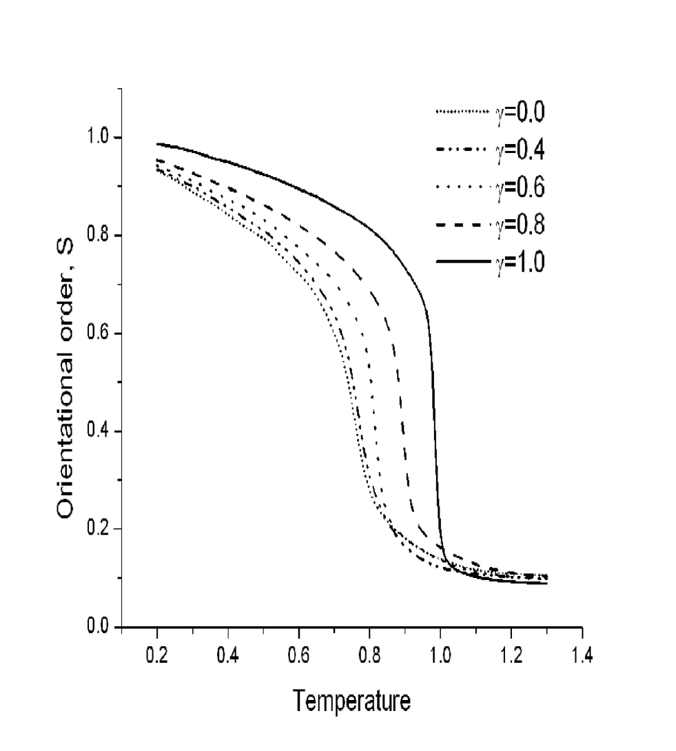
Figure 1: Orientational ordre parameter $S$ versus temperature for various values of the the coupling parameter $\gamma$.

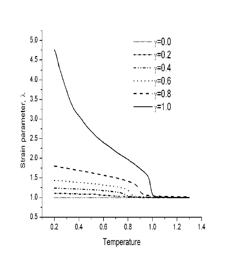
Figure 2: Strain parameter $\lambda$ versus temperature for various values of the the coupling parameter $\gamma$.

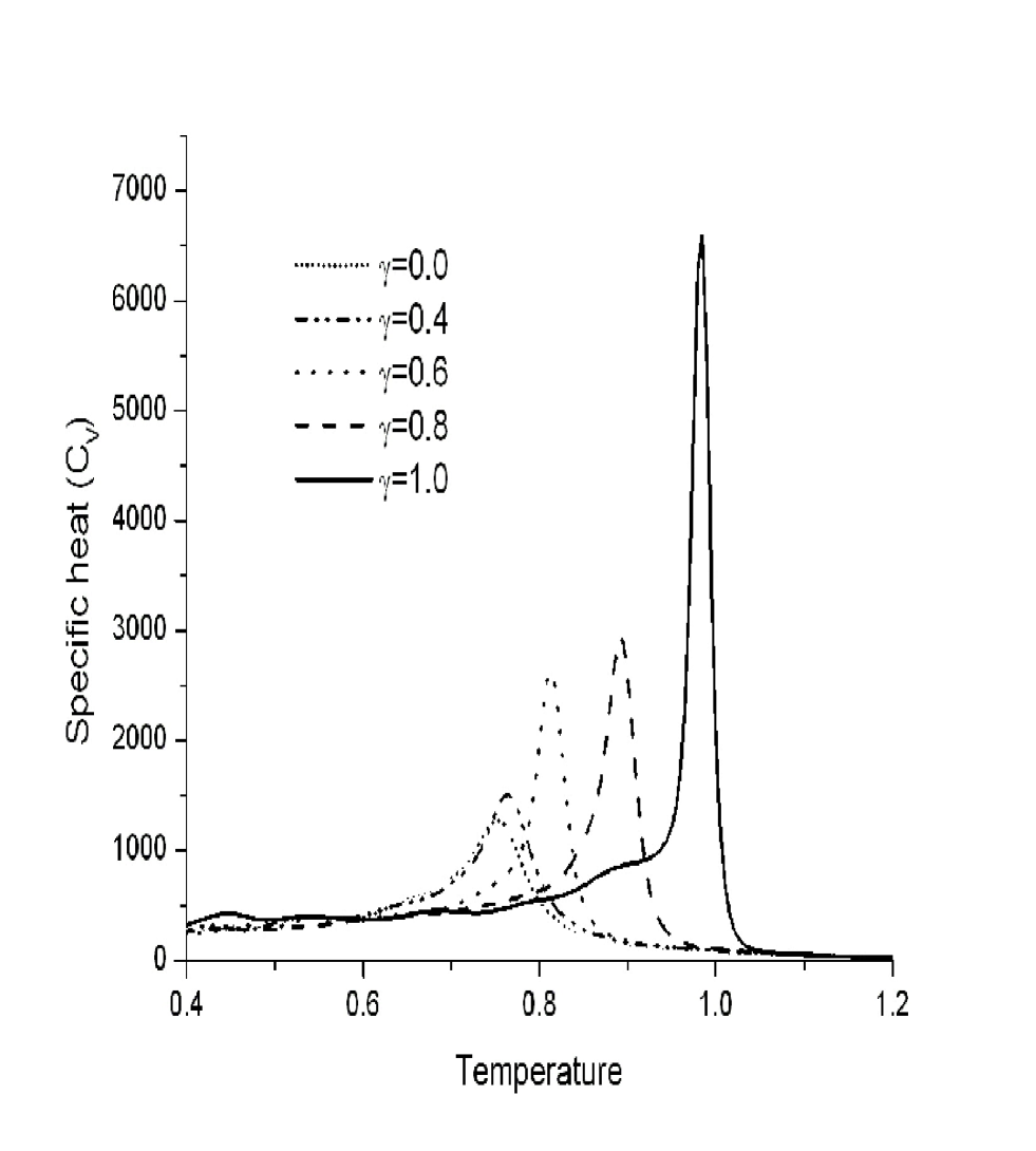
Figure 3: Specific heat ${\rm C}_{V}$ versus temperature for various values of the coupling parameter $\gamma$; ${\rm C}_{V}$ has been obtained from the energy fluctuations.

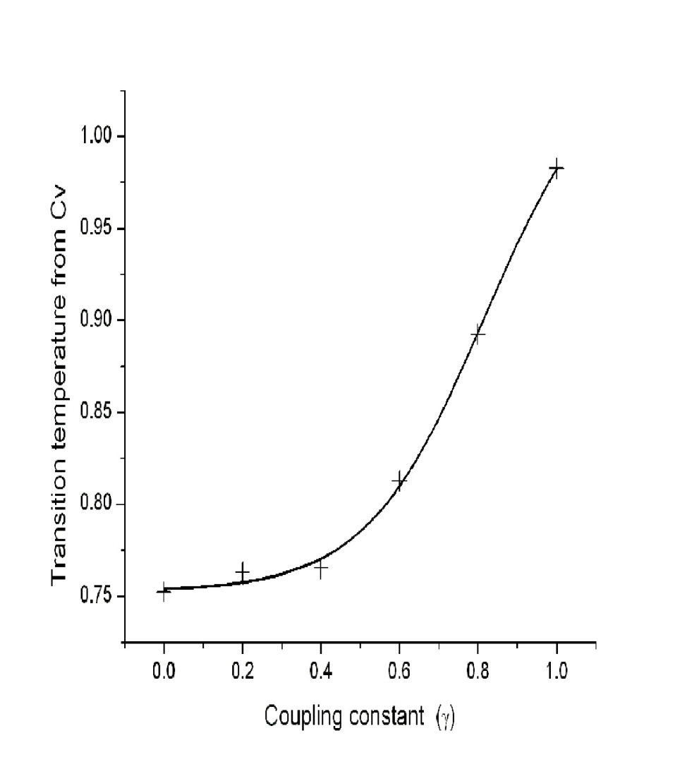
Figure 4: Transition temperature versus the coupling parameter $\gamma$; the temperature at which the specific heat exhibits peak is taken as the transition point.

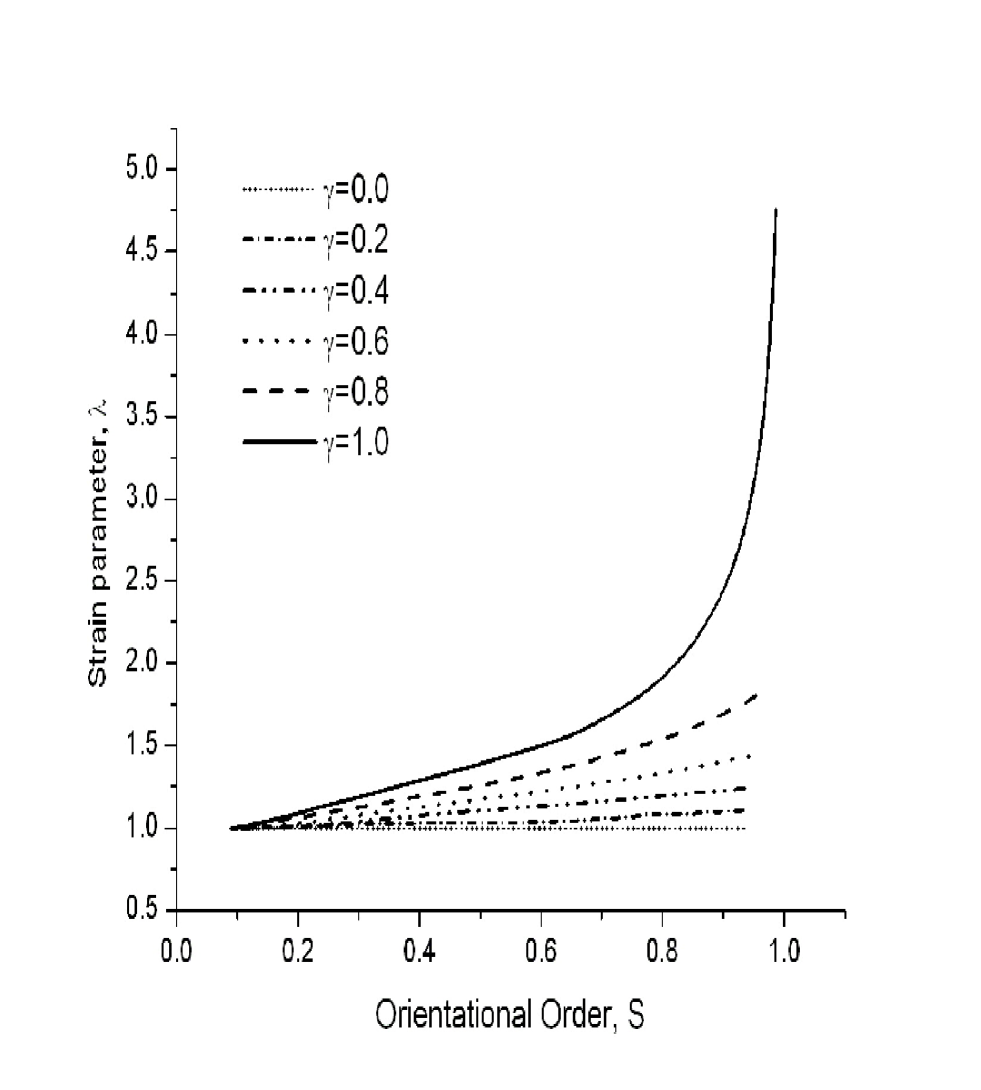
Figure 5: Scaling of Strain ($\lambda$) with orientational order ($S$)

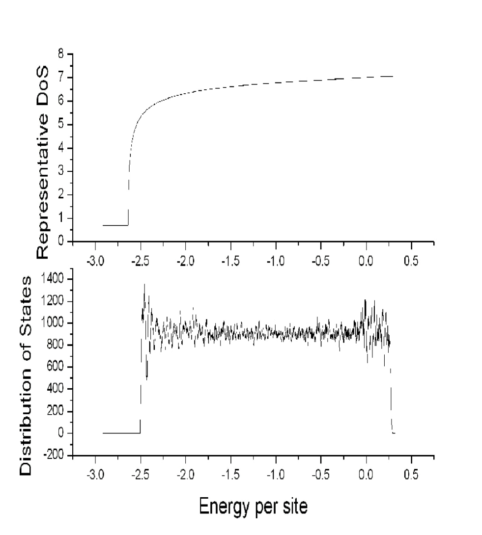
Figure 6: (Top) The $g$ function that approximates the density of states $D$; logarithm of $g$ gives the microcanonical entropy; what is plotted is logarithm of entropy as a function of ewnergy. (Bottom) The histogram of energy of mictrostates sampled during the production run employing entroping sampling with acceptance determined by the density of states depicted in the top.

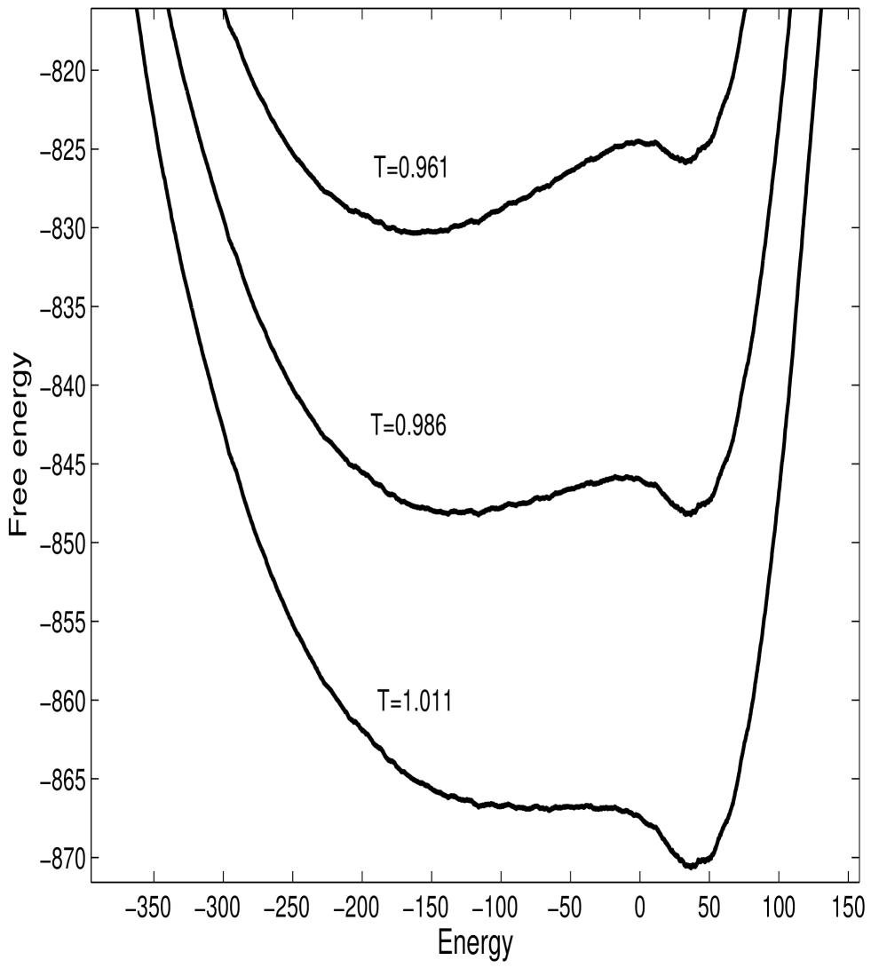
Figure 7: Free energy versus energy for temperatures above, below and at the transition point for the system with $\gamma=1.0$. It is clear that the transition is first order.

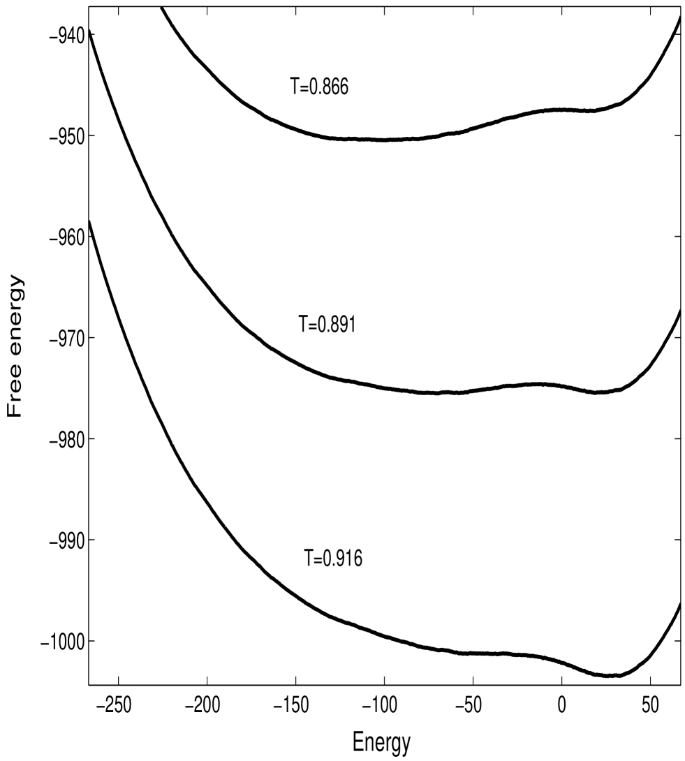
Figure 8: Free energy versus energy for temperatures above, below and at the transition point for the system with $\gamma=0.8$. The barrier height is small; the transition is still first order though weak.

- (1) M. Warner and E. M. Terentjev, Liquid Crystal Elastomers, Clarenden Press, Oxford (2003); M. Warner and E. M. Terentjev, Prog. Polym. Sci. 21, 853 (1996); E. M. Terentjev, J. Phys. : Condens. Matter 11, R239 (1999).
- (2) Y. Mao and M. Warner, Phys. Rev. Lett. 84, 5335 (2000); M. Warner, E. M. Terentjev, R. B. Meyer and Y. Mao, Phys. Rev. lett. 85, 2320 (2000); S. M. Clarke, A. R. Tajbakhsh, E. M. Terentjev and M. Warner, Phys. Rev. Lett. 86, 4044 (2001); Y. Mao and M. Warner, Phys. Rev. Lett. 86, 5309 (2001); P. Pasini, G. Skacej and C. Zannoni, Chem. Phys. Lett. 413, 463 (2005); O. Stenull and T. C. Lubensky, Phys. Rev. E 73, 030701 (R) (2006).
- (3) H. Finkelmann, E. Nishikawa, G. G. Pereira and M. Warner, Phys. Rev. Lett. 87, 015501 (2001).
- (4) J. Küpfer, and H. Finkelmann, Macromol. Chem. Phys. 195, 1353 (1994); H. Finkelmann and H. Wermter, Polym. Mater. Sci. Eng. 82, 319 (2000).
- (5) P. G. de Gennes, C. R. Acad. Sci. Paris 281, 101 (1975); P. G. de Gennes, M. Hubert, and R. Kant, Macromol. Symp. 113, 39 (1997); I. Kun̈dler, H. Finkelmann, Macromol. Chem. Phys. 199, 677 (1998); N. Uchida, A. Onuki, Europhys. Lett. 45, 341 (1999); W. Lehmann, H. Skupin, C. Tolskdorf, E. Gebhard, R. Zentel, P. Kruger, M. Losche and F. Kremer, Nature 410, 447 (2001); Y. Yusuf, Y. Ono, Y. Sumisaki, P. E. Cladis, H. R. Brand, H. Finkelmann and S. Kai, Phys. Rev. E 69, 021710 (2004); Y. Yusuf, P. E. Cladis, H. R. Brand, H. Finkelmann and S. Kai, Chem. Phys. lett. 389, 443 (2004); A. Arcioni, C. Bacchiocchi, I. Vecchi, G. Venditti and C. Zannoni, Chem. Phys. Lett. 396, 433 (2004): D. K.Cho, Y. Yusuf, P. E. Cladis, H. R. Brand, H. Finkelmann and S. Kai, Chem. Phys. Lett. 418, 217 (2006).
- (6) D. L. Thomsen III, P. Keller, J. Naciri, R. Pink, H. Jeon, D. Shenoy, and B.R. Ratna, Macromolecules, 34, 5868 (2001).
- (7) C. -C. Chang, L. -C. Chien and R. B. Meyer, Phys. Rev. E 56, 595 (1997).
- (8) A. R. Tajbaksh and E. M. Terentjev, Euro. Phys. J E 6, 181 (2001).
- (9) D. K. Shenoy, D. L. Thomsen III, A. Srinivasan, P. Keller and B. R. Ratna, Sens. Actuators A 96, 184 (2002); J. Naciri, A. Srinivasan, H. Jeon, N. Nikolov, P. Keller, and B. R. Ratna, Macromolecules 36, 8499 (2003).
- (10) S. Chandrasekhar, Liquid Crystals, Cambridge University Press, Cambridge (1972); G. R. Luckhurst and G. W. Gray (Eds.), The Molecular Physics of Liquid Crystals, Academic Press, New York (1979).
- (11) J. V. Selinger and B. R. Ratna, Phys. Rev. E 70, 041707 (2004).
- (12) Z. Zhang, Phys. Rev. Lett. 69, 2803 (1992).
- (13) D. Jayasri, V. S. S. Sastry and K. P. N. Murthy, Phys. Rev. E 72, 036702 (2005).
- (14) F. Wang, and D. P. Landau, Phys. Rev. Lett. 86 2050 (2001); F. Wang and D. P. Landau, Phys. Rev. E 64 056101 (2001).
- (15) B. A. Berg and T. Neuhaus, Phys. Lett. B 267, 249 (1991); B. A. Berg and T. Neuhaus, Phys. Rev. Lett. 68, 9 (1992); J. Lee, Phys. Rev. Lett. 71 211 (1993); Erratum: 71 2353 (1993)
- (16) P. A. Lebwohl and G. Lasher, Phys. Rev. A 6, 426 (1972).
- (17) J. A. Barker and R. O. Watts, Chem. Phys. Lett. 3 144 (1969)
- (18) N. Metropolis, A. W. Rosenbluth, M. N. Rosenbluth, A. H. Teller and E. Teller, J. Chem. Phys. 21, 1087 (1953).
- (19) M. Cruetz, Phys. Rev. Lett. 43, 553 (1979); R. J. Glauber, J. Math. Phys. 4, 294 (1979); K. Kawasaki, in Phase Transition and Critical Phenomena, Vol. 2, edited by C. Domb and M. S. Green, Academic, London (1972)
- (20) N. Uchida, Phys. Rev. E 62, 5119 (2001).