Slave rotor theory of antiferromagnetic Hubbard model

Abstract

The slave-rotor mean-field theory of Florens and Georges is generalized to the antiferromagnetic phase of the Hubbard model. An effective action consisting of a spin rotor and a fermion is derived and the corresponding saddle-point action is analyzed. Zero-temperature phase diagram of the antiferromagnetic Hubbard model is presented. While the magnetic phase persists for all values of the Hubbard interaction $U$, the single-particle spectral function exhibits a crossover into an incoherent phase when the magnetic moment $m$ (and the corresponding $U$ values) lies within a certain window $m_{c}<m<1-m_{c}$, indicating a possible deviation from the Hartree-Fock theory.

The Hubbard model has received a lot of attention theoretically as a prototypical model for strong electron correlation in low dimensionsHubbard . In particular, much has been learned about the quantum phases and the zero-temperature transitions between them in this model. Brinkman-Rice (BR) theoryBR predicts a metal-to-paramagnetic insulator transition at a finite Hubbard interaction strength $U$, and further refinement by dynamical mean-field theory (DMFT) in recent years supports the original BR pictureDMFT .

Recently Florens and Georges (FG)FG introduced an interesting re-formulation of the Hubbard model. In their slave-rotor (SR) theory, in similar spirit to the slave-boson representation, an electron operator is decomposed as the product of a fermion and a U(1) “slave-rotor” operator. Analysis of the effective mean-field action revealed that a quantum phase transition takes place between metallic and paramagnetic insulating states as $U$ is increased beyond a threshold value $U_{c}$. A good qualitative agreement between FG’s slave-rotor mean-field theory (SRMFT) with the DMFT predictions was achieved while avoiding the use of heavy numerical machinery of the latter method. More recently, SRMFT was employed in the understanding of frustrated Hubbard model on the triangular latticeleelee .

Largely ignored in the above-mentioned theoriesBR ; DMFT ; FG ; leelee ; DMFT-comment is the spin degrees of freedom responsible for the antiferromagnetism. The nesting of the half-filled Fermi surface and the onset of spin density wave are usually treated in the Hartree-Fock (HF) theory while the strong effects of Gutzwiller projection on the HF ground state are ignored. A notable exception in the efforts to go beyond the Hartree-Fock picture to understand the magnetic phase is given by the four-boson formulation of the Hubbard model by Kotliar and Ruckenstein (KR)KR . In KR’s theory strong on-site correlation effects as well as the magnetic order were treated at the mean-field level. Later quantum Monte Carlo study confirmed much of the mean-field conclusions of KRhanke . Both referencesKR ; hanke focused on the overall phase diagram, and the nature of the quasiparticle states in the magnetic phase was not thoroughly discussed. A more recent study on this subjectBD concluded that at strictly zero temperature, as in the Hartree-Fock (HF) picture, the quasiparticles in the antiferromagnetic phase of the Hubbard model remain coherent.

Given the new machinery of SRMFT, we feel that it is worthwhile to re-visit this issue in more detail. In this paper, we present a natural extension of the original SRMFT theory that allows one to treat the magnetic as well as the non-magnetic phase of the Hubbard model. The saddle-point analysis of the effective action for the half-filled model gives two phases, characterized by the coherence/incoherence of the quasiparticles. Further consideration of gauge fluctuation renders the phase transition into a crossover. The magnetic ordering persists for all values of $U$ as in the HF theory.

We start with the Hubbard model

$$H=-t\sum_{ij\sigma}c_{j\sigma}^{\dagger}c_{i\sigma}-\mu\sum_{i\sigma}c^{\dagger}_{i\sigma}c_{i\sigma}+U\sum_{i}c_{i\uparrow}^{\dagger}c_{i\uparrow}c_{i\downarrow}^{\dagger}c_{i\downarrow}$$ (1)

defined on the two-dimensional square lattice. The Hubbard-$U$ term can be decomposed into charge and spin channels in standard fashion

$$c_{i\uparrow}^{\dagger}c_{i\uparrow}c_{i\downarrow}^{\dagger}c_{i\downarrow}=\frac{1}{4}[n_{i\uparrow}+n_{i\downarrow}]^{2}-\frac{1}{4}[n_{i\uparrow}-n_{i\downarrow}]^{2}$$ (2)

with $n_{i\sigma}=c^{\dagger}_{i\sigma}c_{i\sigma}$. The latter term in Eq. (2) was ignored in the study of spinless states by FG.

Florens and Georges introduced a decomposition of the electron operator as $c_{i\sigma}=e^{-i\theta_{i}}f_{i\sigma}$ where the rotor variable $e^{-i\theta_{i}}$ serves to keep track of the charge number at each site, as the creation or annihilation of an electron is accompanied by the phase change $e^{\pm i\theta_{i}}$. Here we propose that a second rotor variable $e^{\pm i\phi_{i}}$ can be introduced for the bookkeeping of spin numbers. The representation of the electron operator we propose is

$$c_{i\sigma}=e^{-i\theta_{i}-i\sigma\phi_{i}}f_{i\sigma}.$$ (3)

The factor $\sigma=\pm 1$ is used to distinguish the creation of up and down spins along the $\hat{z}$-axis. Although we are focusing on the U(1) case here, a fully SU(2)-invariant representation of the spin sector is also possible.

After the substitution made in Eq. (3), the local charge $\sum_{\sigma}c^{\dagger}_{i\sigma}c_{i\sigma}$ and the local $z$-spin $\sum_{\sigma}\sigma c^{\dagger}_{i\sigma}c_{i\sigma}$ appearing in the decomposition of the Hubbard term are replaced by the conjugate operators of $(\theta_{i},\phi_{i})$, which we denote $(L_{i},M_{i})=(-i\partial/\partial\theta_{i},-i\partial/\partial\phi_{i})$. The Hubbard Hamiltonian takes on the expression

$$H={U\over 4}\sum_{i}L_{i}^{2}-{U\over 4}\sum_{i}M_{i}^{2}-\mu\sum_{i\sigma}f^{\dagger}_{i\sigma}f_{i\sigma}$$

$$-t\sum_{ij\sigma}f^{\dagger}_{j\sigma}e^{i(\theta_{j}-\theta_{i})+i\sigma(\phi_{j}-\phi_{i})}f_{i\sigma}$$ (4)

supplemented by the constraints $L_{i}=\sum_{\sigma}f^{\dagger}_{i\sigma}f_{i\sigma}$ and $M_{i}=\sum_{\sigma}\sigma f^{\dagger}_{i\sigma}f_{i\sigma}$ at every siteFG . The corresponding action can also be derived straightforwardly:

$$L=\sum_{i\sigma}f_{i\sigma}^{*}(\partial_{\tau}-\mu)f_{i\sigma}-t\sum_{ij\sigma}f_{j\sigma}^{*}e^{i(\theta_{j}-\theta_{i})+i\sigma(\phi_{j}-\phi_{i})}f_{i\sigma}$$

$$+\sum_{i}\Bigl{[}\frac{U}{4}L_{i}^{2}-iL_{i}\partial_{\tau}\theta_{i}+i\lambda_{i}(L_{i}-\sum_{\sigma}{f}_{i\sigma}^{*}{f}_{i\sigma})\Bigr{]}$$

$$+\sum_{i}\Bigl{[}-\frac{U}{4}M_{i}^{2}-iM_{i}\partial_{\tau}\phi_{i}+i\eta_{i}(M_{i}-\sum_{\sigma}\sigma{f}_{i\sigma}^{*}{f}_{i\sigma})\Bigr{]}.$$

(5)

A pair of Lagrange multipler fields $(\lambda_{i},\eta_{i})$ has been introduced to impose the constraints. The original theory of FG is based on this Lagrangian, without the terms pertaining to the spin decomposition such as $M_{i}$, $\phi_{i}$, and $\eta_{i}$. Our formulation thus generalizes the scheme of FG in a natural way to include magnetic order.

To proceed further, we ignore the terms pertaining to the charge sector as they are already discussed by FG. Leaving out the terms containing $(\theta_{i},L_{i},\lambda_{i})$, the next step is to integrate out $M_{i}$ from the action. Because of the negative norm in $M_{i}^{2}$ (third line of Eq. (5)), we use the following identity of the Gaussian integration

$$\int_{-\infty}^{\infty}dM\int_{-\infty}^{\infty}d\eta~{}~{}e^{{1\over 2}M^{2}+iaM-i\eta(M-s)}$$

$$=\int_{-\infty}^{\infty}d\eta\int_{-\infty}^{\infty}dM~{}~{}e^{-{1\over 2}M^{2}-aM-i\eta(M+is)}$$ (6)

to first re-write the action (5) with the positive norm for $M_{i}^{2}$. The integration over $M_{i}$ of the modified action can then proceed to give

$$L=\sum_{i\sigma}f_{i\sigma}^{*}(\partial_{\tau}-\mu-\sigma\eta_{i})f_{i\sigma}+{1\over U}\sum_{i}(\eta_{i}-i\partial_{\tau}\phi_{i})^{2}$$

$$~{}~{}~{}-t\sum_{ij\sigma}f_{j\sigma}^{*}e^{i\sigma(\phi_{j}-\phi_{i})}f_{i\sigma}.$$ (7)

The final manipulation involves the shift $\eta_{i}\rightarrow\eta_{i}+i\partial_{\tau}\phi_{i}$ that gives

$$L=\sum_{i\sigma}f_{i\sigma}^{*}(\partial_{\tau}\!-\!\mu\!-\!\sigma\eta_{i}\!-\!i\sigma\partial_{\tau}\phi_{i})f_{i\sigma}+{1\over U}\sum_{i}\eta_{i}^{2}$$

$$~{}~{}~{}-t\sum_{ij\sigma}f_{j\sigma}^{*}e^{i\sigma(\phi_{j}-\phi_{i})}f_{i\sigma}.$$ (8)

This concludes the formal derivation of the effective action for the spin-ful Hubbard model within the slave-rotor framework. Without the phase fluctuations in Eq. (8) this effective action at the saddle-point level is equivalent to the HF theory of the Hubbard model.

To explore the consequences of phase fluctuations in the action (8), we replace $\eta_{i}$ by its saddle-point value $\overline{\eta}_{i}$ given by

$$\overline{\eta}_{i}={U\over 2}\langle\sum_{\sigma}\sigma f^{*}_{i\sigma}f_{i\sigma}\rangle\equiv{U\over 2}m_{i},$$ (9)

which is identical to the saddle-point equation in the absence of the phase fluctuation. We will write $\eta_{i}$ to refer to this average value in the rest of the paper.

One can decompose the hopping term in Eq. (8) by a pair of Hubbard-Stratonovich (HS) fields $(\alpha_{ij},\beta_{ij})$leelee , resulting in the effective Lagrangian

$$L=L_{0}+L_{f}+L_{\phi},$$

$$L_{0}=t\sum_{\langle ij\rangle}(\alpha_{ij}\beta_{ij}^{*}+\alpha_{ij}^{*}\beta_{ij})+{1\over U}\sum_{i}\eta_{i}^{2},$$

$$L_{f}=\sum_{i\sigma}f_{i\sigma}^{*}(\partial_{\tau}\!-\!\mu\!-\!\sigma\eta_{i}\!-\!i\sigma\partial_{\tau}\phi_{i})f_{i\sigma}$$

$$~{}~{}~{}~{}-t\sum_{\langle ij\rangle}(f^{*}_{j\uparrow}\beta_{ij}f_{i\uparrow}+f^{*}_{j\downarrow}\beta_{ij}^{*}f_{i\downarrow}+c.c.),$$

$$L_{\phi}=-t\sum_{\langle ij\rangle}(e^{-i\phi_{j}}\alpha_{ij}e^{i\phi_{i}}+c.c.).$$ (10)

At the saddle-point level, the HS parameters take on the average values $\alpha_{ij}=\langle f^{*}_{i\uparrow}f_{j\uparrow}+f^{*}_{j\downarrow}f_{i\downarrow}\rangle$, $\beta_{ij}=\langle e^{-i\phi_{i}}e^{i\phi_{j}}\rangle$. Assuming real and uniform mean-field solutions $\alpha_{ij}=\alpha$, $\beta_{ij}=\beta$, and staggered effective magnetic fields $\eta_{i}=(-1)^{i}\eta$, $m_{i}=(-1)^{i}m$, we arrive at the mean-field effective action:

$$L_{MF} = L_{f}+L_{\phi},$$

$$L_{f} = \sum_{i\sigma}f_{i\sigma}^{*}(\partial_{\tau}\!-\!\mu\!-\!\sigma(-1)^{i}\eta)f_{i\sigma}-t\beta\sum_{ij\sigma}f^{*}_{j\sigma}f_{i\sigma}$$

$$L_{\phi} = -2t\alpha\sum_{\langle ij\rangle}\cos[\phi_{j}-\phi_{i}]-i\sum_{i}m_{i}\partial_{\tau}\phi_{i}$$

We assumed the case of no broken time-reversal symmetry, $\langle\partial_{\tau}\phi_{i}\rangle=0$. The fermion action is in the standard HF form except for the renormalization of the bandwidth $t\rightarrow\beta t$. At zero temperature the fermion sector thus always remains in the magnetic phase with a gap to quasiparticle excitations. The boson action, on the other hand, is the standard XY action modified by the Berry phase term $i\sum_{i}m_{i}\partial_{\tau}\phi_{i}$. We analyze each of the mean-field actions derived in Eq. (LABEL:mean-field-for-S), beginning with the fermion sector.

In analyzing the fermionic mean-field action we confine our attention to half-filling for which $\mu=0$. The mean-field conditions for $\eta$ and $\alpha$ at $T=0$ read

$$\eta=U\eta\sum^{\prime}_{k}{1\over E^{f}_{k}},~{}~{}\alpha={2\over zt}\sum^{\prime}_{k}\epsilon_{k}\times{\beta\epsilon_{k}\over E^{f}_{k}}.$$ (12)

Here $\epsilon_{k}=-t\sum_{j\in i}e^{ik\cdot(r_{j}-r_{i})}$ ($j$ runs over all nearest neighbors of $i$) is the bare band in the absence of exchange splitting introduced by non-zero $\eta$, and $z$ is the lattice coordination number. The $k$-sum in both equations is over the reduced Brillouin zone and $E^{f}_{k}=\sqrt{(\beta\epsilon_{k})^{2}+\eta^{2}}$ is the fermionic energy with a gap set by $\eta$.

The bosonic action derived in Eq. (LABEL:mean-field-for-S) is invariant under $m\rightarrow-m$ or $m\rightarrow 1-m$ followed by a shift of one lattice spacing. The Berry phase term vanishes for $m=0$ and $m=1$ leaving only the classical XY model with an ordered phase $\phi_{i}=\phi_{0}$ at zero temperature. One might thus expect that small deviations such as $m\approx 0$ and $m\approx 1$ still gives the ordered phase while $m\approx 0.5$ introduces enough perturbation to induce phase disordering. We present a calculation which confirms this expectation.

Following the treatment of FGFG we introduce the uni-modular field $Y_{i}$ to make the replacement $e^{i\phi_{i}}\equiv Y_{i}$. An additional Lagrange multiplier $q_{i}$ is required to impose the uni-modular constraint. This extension allows us to examine the bosonic action at the saddle-point level. The effective boson Lagrangian written in terms of $Y_{i}$ reads

$$L_{Y}=-t\alpha\sum_{ij}Y^{*}_{j}Y_{i}+i\sum_{i}q_{i}(Y^{*}_{i}Y_{i}-1)$$

$$~{}~{}~{}~{}-{m\over 2}\sum_{i}(-1)^{i}[Y^{*}_{i}\partial_{\tau}Y_{i}-(\partial_{\tau}Y^{*}_{i})Y_{i}]$$

$$=\sum^{\prime}_{k\nu}Y^{*}_{k\nu}\left(q+\alpha\epsilon_{k}\right)Y_{k\nu}+\sum^{\prime}_{k\nu}Y^{*}_{k+Q\nu}\left(q-\alpha\epsilon_{k}\right)Y_{k+Q\nu}$$

$$~{}~{}~{}~{}-m\sum^{\prime}_{k\nu}i\nu(Y^{*}_{k+Q\nu}Y_{k\nu}+Y^{*}_{k\nu}Y_{k+Q\nu}),$$ (13)

with $Q=(\pi,\pi)$. In writing down the Fourier form we assumed a uniform mean-field solution $i\langle q_{i}\rangle=q$. The bosonic $k$-sum is also over the reduced Brillouin zone. The boson part can be diagonalized using a pair of operators $(\gamma_{1k\nu},\gamma_{2k\nu})$ related to $(Y_{k\nu},Y_{k+Q\nu})$ by

$$Y_{k\nu} = {1\over\sqrt{2}}(\cosh\theta_{k}-\sinh\theta_{k})(\gamma_{1k\nu}+\gamma_{2k\nu})$$

$$Y_{k+Q\nu} = {1\over\sqrt{2}}(\cosh\theta_{k}+\sinh\theta_{k})(\gamma_{1k\nu}-\gamma_{2k\nu}).$$ (14)

After taking $\cosh 2\theta_{k}=q/E^{b}_{k}$, $\sinh 2\theta_{k}=\alpha\epsilon_{k}/E^{b}_{k}$, and $E^{b}_{k}=\sqrt{q^{2}-(\alpha\epsilon_{k})^{2}}$, one gets

$$L_{Y}=-im\sum^{\prime}_{k\nu}\nu(\gamma^{*}_{1k\nu}\gamma_{1k\nu}-\gamma^{*}_{2k\nu}\gamma_{2k\nu})$$

$$~{}~{}~{}~{}+\sum^{\prime}_{k\nu}E^{b}_{k}(\gamma^{*}_{1k\nu}\gamma_{1k\nu}+\gamma^{*}_{2k\nu}\gamma_{2k\nu}).$$ (15)

The boson spectrum $E^{b}_{k}$ is gapped if $q-\alpha{D}>0$ while $q-\alpha{D}=0$ leads to the condensation of $Y$. Here $D=zt$ is half the bare bandwidth. Two additional relations are obtained at $T=0$ from the constraints $\langle Y^{*}_{i}Y_{i}\rangle=1$ and $\beta=\langle Y^{*}_{i}Y_{j}\rangle$:

$${m\over q}=\sum^{\prime}_{k}{1\over E^{b}_{k}},~{}~{}~{}\beta={\alpha\over zt}\sum^{\prime}_{k}{\epsilon_{k}^{2}\over m}{1\over E^{b}_{k}}.$$ (16)

Solving Eqs. (12) and (16) simultaneously renders the self-consistent parameters $(\alpha,\beta,m,q)$ for a given $U/D$. The Bose condensation occurs when $q=\alpha D$, which gives $m_{c}\approx 0.69$.

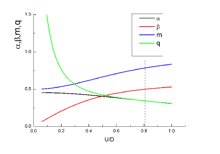
Figure 1: (color online) Plot of mean-field parameters $(\alpha,\beta,m,q)$ for $U/D$ obtained from solving Eq. (Slave rotor theory of antiferromagnetic Hubbard model). $q$ equals $\alpha D$ at $(U/D)_{c}\approx 0.81$ indicated by a dashed vertical bar.

To get a better idea on the analytical structure of the set of self-consistent equations obtained above, we first re-write Eqs. (12) and (16) as the integration over the energy with a certain density of states $D(\epsilon)$, and approximate it with a constant value, $D(\epsilon)=1/(2D)$. The mean-field equations are then given by

$$m={2\beta D/U\over\sinh[2\beta D/U]}, \alpha={\sinh[4\beta D/U]-4\beta D/U\over 4\sinh^{2}[2\beta D/U]}$$

$$q={\alpha D\over\sin[2m\alpha D/q]}, \beta={4m\alpha D/q-\sin[4m\alpha D/q]\over 8m\sin^{2}[2m\alpha D/q]}.$$

The Bose condensation occurs at $m_{c}=\pi/4\approx 0.8$ ($(U/D)_{c}\approx 0.81$), similar to the earlier estimate. The plot of all four self-consistent parameters with varying $U/D$ using Eq. (Slave rotor theory of antiferromagnetic Hubbard model) is shown in Fig. 1.

The set of mean-field equations (Slave rotor theory of antiferromagnetic Hubbard model) yields $m=1/2$, not $m=0$ as in the HF theory, when $U/D\rightarrow 0$. We believe this is an artifact of the replacement $e^{i\phi_{i}}\rightarrow Y_{i}$. The boson action in Eq. (LABEL:mean-field-for-S), being equivalent to the XY model, must show ordered phase at $m=0$ and $m=1$, and the only chance of a disordered phase occurs for intermediate $m$ values. Combining this general argument with the mean-field analysis in terms of $Y$, we conclude that the incoherent phase exists within the window $1-m_{c}\lesssim m\lesssim m_{c}$ with $m_{c}\approx 0.8$. In this intermediate phase the boson gap $\Delta_{b}=\sqrt{q^{2}-(\alpha D)^{2}}$ remains finite. Due to the gap, the spectral function of the composite electron operator is incoherentFG-comment . The region outside this value gives Bose condensation, or the coherent quasiparticles. Meanwhile the magnetic sector remains ordered for all $U/D$ as in the HF theory. For comparison we recall that in the paramagnetic Hubbard modelFG , SRMFT gave Bose condensation for small-$U$: $0<U/D<(U/D)_{c}$.

So far we performed saddle-point analysis and obtained a mean-field picture showing a second order phase transition (with the boson gap as the order parameter) for the spin phase field $\phi_{i}$ in the intermediate values of $U/D$. It is natural to ask the stability of the mean-field picture against the gauge field $a_{ij}$ that appears in the phase fluctuations of the hopping order parameters, $\alpha_{ij}=\alpha{e}^{ia_{ij}}$ and $\beta_{ij}=\beta{e}^{ia_{ij}}$, where $\alpha$ and $\beta$ are the mean field values obtained before. It should be noted that the U(1) spin-gauge field $a_{ij}$ is compact, thus allowing instanton excitationsPolyakov . From the seminal work of Fradkin and ShenkerFS_Instanton we know that there can be no phase transition between the Higgs and confinement phases due to instanton proliferation, and only a crossover behavior is expected. In the present problem the phase-coherent state corresponds to the Higgs phase while the phase-incoherent state coincides with the confinement phase. Applying Fradkin and Shenker’s result to the present problem, we conclude that the second order phase transition turns into a crossover between the coherent and incoherent phases. The magnetic order parameter, being a gauge-invariant quantity, remains unaffected by the gauge fluctuation.

In summary we have developed an extension of the slave-rotor theory of Florens and Georges to the magnetically ordered phase by introducing a second rotor variable pertaining to the spin degrees of freedom. On performing a saddle point analysis we uncover an incoherent-to-coherent crossover within the half-filled antiferromagnetic phase of the Hubbard model at zero temperature. The incoherent phase exists in the intermediate values of $U/D$ between weak and strong coupling limits. Given the common conception that the magnetically ordered phase of the Hubbard model at $T=0$ is well understood within the HF theory, the possibility we suggest in this paper is tantalizing. The formalism developed in this work may also be of use for understanding other exotic magnetic systems.

HJH was supported by Korea Research Foundation through Grant No. KRF-2005-070-C00044.

References

• (1) For a compilation of relatively recent results, see The Hubbard Model: Its Physics and Mathematical Physics, Edited by D. Baeriswyl (Plenum Press, New York, 1995).
• (2) W. F. Brinkman and T. M. Rice, Phys. Rev. B 2, 4302 (1970).
• (3) A. Georges, G. Kotliar, W. Krauth, and M. J. Rozenberg, Rev. Mod. Phys. 68, 13 (1996).
• (4) Serge Florens and Antoine Georges, Phys. Rev. B 66, 165111 (2002); Phys. Rev. B 70, 035114 (2004).
• (5) S.-S. Lee and P. A. Lee, Phys. Rev. Lett. 95, 036403 (2005).
• (6) DMFT study of the antiferromagnetic Hubbard model has been carried out, for instance, by M. J. Rozenberg, G. Kotliar, and X. Y. Zhang, Phys. Rev. B 49, 10181 (1994), without an explicit discussion of the quasiparticle coherence in the antiferromagnetic regime.
• (7) Gabriel Kotliar and Andrei E. Ruckenstein, Phys. Rev. Lett. 57, 1362 (1986).
• (8) L. Lilly, A. Muramatsu, and W. Hanke, Phys. Rev. Lett. 65, 1379 (1990).
• (9) K. Borejsza and N. Dupuis, Phys. Rev. B 69, 085119 (2004).
• (10) In FG’s work as in ours, the Bose condensation marks the coherence of quasiparticles. A finite boson gap implies that the composite object’s spectral function is incoherent. For an explicit calculation of the electron spectral function see Ref. FG, .
• (11) A. M. Polyakov, Gauge Fields and Strings, Ch. 4 (Harwood Academic Publishers, 1987).
• (12) E. Fradkin and S. H. Shenker, Phys. Rev. D 19, 3682 (1979).